Personalized bank campaign using artificial neural networks

(1)

MAA

Master Program in Advanced Analytics

Personalized Bank Campaign Using Artficial Neural

Networks

Simota Asimina

Internship report presented as partial requirement for

obtaining the Master’s degree in Advanced Analytics

NOVA Information Management School

Instituto Superior de Estatística e Gestão de Informação Universidade Nova de Lisboa

(2)

ii

NOVA Information Management School

Instituto Superior de Estatística e Gestão de Infrormação

Universidade Nova de Lisboa

PERSONALIZED BANK CAMPAIGN

USING ARTIFICIAL NEURAL NETWORKS

by

Asimina Simota

Internship report presented as partial requirement for obtaining the Master´s degree in Advanced Analytics.

Advisor: Leonardo Vanneschi

(3)

iii

ACKNOWNLEDGEMENTS

I would like to thank Professor Leonardo Vanneschi for the amazing lectures and his magic way to make the most complex algorithms completely comprehensive.

Furthermore, I would like to express my gratitude to Mr. Theoklitos Vadileiadis for his guidance and for inspired me to apply in this Master the degree.

Special thanks to my friend Euaggelia Koumoutsou, who always motivating me through great discussions.

Moreover, I am thankful to my sisterly friend, Ioanna Foka, for all the support during this year.

Finally, I would like to thank for all they have done for me, my beloved and amazing family. Soula, Kostas, Spiros, Areti, Tzema, Giorgos and Poker.

I dedicate this thesis to my grandparents.

(4)

iv

ABSTRACT

Nowadays, high market competition requires Banks to focus more at individual customers´ behaviors. Specifically, customers prefer a personal relationship with the finance institution and they want to receive exclusive offers. Thus, a successful cross-sell and up- cross-sell personalized campaign requires to know the individual client interest for the offer. The aim of this project is to create a model, that, is able to identify the probability of a customer to buy a product of the bank. The strategic plan is to run a long-term personalized campaign and the challenge is to create a model which remains accurate during this time. The source datasets consist of 12 dataMarts, which represent a monthly snapshot of the Bank’s dataWarehouse between April 2016 and March 2017. They consist of 191 original variables, which contain personal and transactional information and around 1.400.000 clients each. The selected modeling technique is Artificial Neural Networks and specifically, Multilayer Perceptron running with Back-propagation. The results showed that the model performs well and the business can use it to optimize the profitability. Despite the good results, business must monitor the model´s outputs to check the performance through time.

Keywords:

(5)

v

LIST OF FIGURES

Figure 1: Project Methodology ... 6

Figure 2: Data Understanding and Preparation Process ... 9

Figure 3: SAS code for Target Creation ... 12

Figure 4: Target percentage per month and model Time window ... 13

Figure 5: Explanatory Analysis... 14

Figure 6: ANN Model Process ... 20

Figure 7: General Neuron Process ... 22

Figure 8: Feedforward and Feedback Networks ... 23

Figure 9: Model Architecture ... 27

Figure 10: Confusion Matrices of Training and Test sets ... 29

Figure 11: Evaluation Metrics ... 29

Figure 12: Evaluation Results Train and Test sets ... 30

Figure 13: ROC curves Train and Test sets ... 31

Figure 14: Comulative % Response Curve ... 32

(7)

vii

LIST OF TABLES

Table 1 : Basic Features of DM Methodologies... 5

Table 2: Original Variables ... 10

Table 3: Generated Variables ... 11

Table 4: Common Outlier Treatments ... 16

Table 5: Common Transformations ... 17

Table 6: Variable Selection Common Strategies ... 18

Table 7: Input Variables... 19

Table 8: Error of different Learning Rate and Momentum values ... 25

Table 9: final Artificial Neural Network Parameters ... 26

(8)

viii

LIST OF ABREVIATIONS AND ACRONYMS

CRISP-DM Cross

–

Industry Standard Process for Data Mining ANN Artificial Neural Network

(9)

1

1. INTRODUCTION

1.1 PROBLEM IDENTIFICATION

Satisfying customers in today’s competitive market has never been more challenging. Clients has become more demanding and they want products and services fitted to their specific needs. They want to feel that the offering is personally addressed to them (Girish, 2010). To answer this need, businesses generated different tools and techniques over time, but the provided information was not necessarily what the client expected. To gain deeper insights into customer trends, businesses have been supporting the evolution of the predictive analytics field, which makes them able to target the right offers at the right time, as well as being changing depending on the requirements throughout the customer lifecycle.

When a business wants to apply a marketing campaign, predictive models provide exclusive information about customer’s future behavior preferences and needs. Firms investing in predictive analytics are almost twice as likely to identify the most probable buyers and make appropriate offers to them (Aberdeen, 2011). Specifically, companies that use data analytics are able create more accurate segments on clients and target them with offers, getting a response rate around 82%. The same percentage without predictive modeling is less than 50%. Specifically, in personalized targeted campaigns, where each client treated as individual and receive specific offers, these percentages are 68% and 38 % respectively. It turns out, that companies who follow this strategy, not only increase revenues but also get advantages in terms of customer retention and satisfaction (SPSS, 2004).

Banks nowadays face exactly the same challenge. They need to analyze customer individual preferences to attract new clients and increase revenue from the already existent. Churn detection, default propensity, Cross-sell and up-sell opportunities are the most common customer analytics that are served by predictive modeling. Currently, the overall contribution of predictive analytics in banking is still in a transitional stage but until 2020 banks are expected to be the leaders in applied predictive models (Framingham, 2017). Specifically, the global bank industry revenues coming from data analytics they will increase from 10% in 2013, to around 40% the next years (Simonson and Jain,2014).

1.2 STUDY OBJECTIVE

The bank understudy decided to apply a long-term personalized cross -sell and up -sell campaign to the customers that already interact with it. In up-selling, the purpose is to upgrade the product that the client already owes, while in cross-selling, business tries to sell different products based on what the client already purchased. In some specific

(10)

2

cases, the client can purchase twice and more times the same product, and here, this is also defined as cross-selling. The aim of this study is to identify the clients that they have strong willing to accept a product offer. The cross-sell and up-sell application are business responsibility and they are not included in the project.

The prediction plan involves 2 main steps. (1) contact a client with an offer that he probably wants, (2) do that, the moment that he is more likely to buy it. In the first part, predictive analytics will be applied to generate a list with all the clients and their probability to buy each product of the bank. Clients with high values they will receive a promotion for the business. Of, course there are specific cases that someone is forbidden to purchase a product and thus not probabilities are extracted. This issue will be discussed later in the analysis, but for example a client who owes a life insurance he is not allowed to get another one. From technical point of view, a function will be created that returns future behavior by combining variables from the bank database. The second part of the strategic plan characterizes mainly the imbalances in customer behavior. Clients use to change preferences over time and those who are not potential buyers now, maybe in the future want to purchase the product. Business needs to watch these changes and send an offer the moment that client is more likely to buy. To do this, the probabilities need to be reconstructed regularly in order to present realistic and correct results. The main challenge of predictive analytics, and also in this project, is to generate a function that can return accurate results for a long-time period.

For this study 26 models are created, one for each banking product. For confidential reasons, only one product is presented, but the process is the same for all of them.

(11)

3

2. LITERATURE REVIEW

The core key of marketing campaigns is to increase customers satisfaction. Common marketing policies that applied in business are better services, personalized offers, decreasing prices, diversity on products, and personal relationship with the clients. Specifically, in bank sector, promotion campaigns are used more often than the past years and they seem to have a great impact in customers preferences (Mylonakis, 2008). Personalized offers are currently the increasing promotion trend. An interesting survey of (Ernst & Young, 2010) showed, that in Bank sector personalization has a strong impact in customers satisfaction, and thus, affects their willing to buy. Specifically, around 50% of the sample consider personal offers as medium important, whereas, more than 20% gives them a high importance value. Another one survey regarding banks and customer relationship (Personetics, 2016), showed that around 40% of the clients believe, that their bank must know them personally and try to give them the service that they want. Predictive analytics is today the main business tool to understand the customers individually and reach them personally (Girish, 2010). They are a subfield of the general category to extract knowledge from databases called data mining (Zhang S., Zhang C. and Wu, 2004).

Predictive modeling is a common technique applied by organizations to make prediction about unknown events. Particularly, it is a de facto standard in developed markets, where the volume of studied data has a substantial volume (Lee and Guven, 2012). Predictive analytics have several areas of application such as archaeology, health care and businesses. In archelogy, it can be used to allocate human activities in specific locations and study their behaviors (Gillam,2016). In health care, predictive modeling supports the clinical diagnosis, it helps to improve the accuracy of a diagnostic test and it gives warnings about an epidemic outbreak (Palem, 2017). In business, the application it is also wide. It can be used to support fraud detection, claims and risk management, churn identification and personalized marketing campaigns (Batty, et al., 2010). In the current case, predictive analytics will be used to identify what is the banking product that the client wants the most and what is the probability to buy it. Each client will receive an individual offer based on these results.

The process of predictive modeling is to get historical and current data and identify a mathematical relationship between a target variable and explanatory variables, using mainly statistical and mathematical techniques (Dickey, 2012). There are two approaches to solve this problem (1) Statistical methods and (2) Machine learning algorithms. Statistical methods are the oldest approaches and they characterized by several requirements (Han, Phan and Whitson, 2016). Specifically, they often use only few features to construct a model, they need input data with certain characteristics and they involve many statistical assumptions. Such as methods are, the ordinary multivariate linear regression and the logistic regression. Contrary, Machine learning methods tend to return more accurate predictions, accept a high volume of data, deal with several data types (structured, unstructured), have less assumptions and being

(12)

4

more automated (Han, Phan and Whitson, 2016). The core of machine learning algorithms is to introduce them data without giving a specific solution structure, and them being able to identify relationships. There are 3 major learning types (Krenker, Bester and Kos): (1) Supervised learning, (2) Reinforcement learning and (3) Unsupervised learning.

Supervised learning: a set of explanatory variables and a desired output variable is given. The aim of the learning algorithm is to identify a mathematical relationship that will lead to the desired output through the explanatory variables. It is used in predictions.

Reinforcement learning: is a special case of supervised learning where instead of a desired output, an information regarding good or bad algorithmic performance is given. Unsupervised learning: only the explanatory variables are provided. The aim of the algorithm is to identify relationships among input data and discover unknown patterns of them. The most common methods are cluster analysis and dimensionality reduction (Ghahramani, 2004).

There are several ML algorithms provided by literature to support problem solving. They can differentiate by the adapted learning process and their problem task specialization (Lantz, 2015). Common tasks are the numeric prediction, classification, clustering and pattern detection. In this case, bank wants to predict the customer´s willing to purchase a product based on his historical behaviors and preferences. Thus, a classification problem is defined and the selected algorithm is the Artificial Neural Networks. ANN algorithms have key advantages and they play an increasingly important role in the financial industries (Epidemiol, 1997). They can detect complex nonlinear relationship between dependent and independent variables, they require less statistical assumptions and they offer a great scale of training algorithms.

Artificial neuron networks are inspired by the structure and functions of the biological human brain (Hagan, et al., 2014). They basically transfer data through some interconnected elements, called artificial neurons. During these transfers, data are influenced by some parameters called weights and bias. Parameters and data are combined through functions to serve the model purpose. The main function is called activation function and defines the reaction of the neuron to the input information. ANNs are robust, fault tolerant and they can effectively work with qualitative and incomplete data (Hung and Kao, 2001). They require less statistical power and they are great detectors of nonlinear relationships between dependent and independent variables (Teshnizi and Ayatollahi, 1996). Neural Networks despite their advantages, they have two natural limitations: (1) External factors and (2) Internal Factors (Kezdoglou, 1999). External factors are the quality of the input dataset. Internal factors are the choices of an appropriate network structure, such as connections, weights, number of iterations, and process function. External and Internal factors will be deeply described in 4th_{and 5}th_{section respectively.}

(13)

5

3. METHODOLOGY

This project made under the CRISP-DM methodology. 3.1 BACKROUND AND SELECTION

There are several methodologies and model processes proposed by literature to develop a datamining process. Their difference can be based on details like big data specialization or in the exclusion of a whole task such as business understanding. (Fayyad, Shapiro and Smyth 1996) mentioned that the main difference between a methodology and a process model is that the last does not include actions. Methodology must establish not only the steps to be taken for a predictive project but also how this task must be carried out. Thus, methodologies and process models can be combined. KDD process, CRISP -DM and SEMMA methodologies are the most important. The first 2 are the basis for major methods. Especially CRISP-DM is the de facto standard (Chapman et all., 2000) for a complete data mining solution.

The following table summarizes the methods characteristics based on (Mariscal, Marban and Fernandez, 2010). It presents the 3 most used approaches KDD, CRISP-DM, SEMMA and some alternatives of CRISP -DM. CIO´s, CRISP-DM 2.0, RAMSYS and DMIE.

Table 1 : Basic Features of DM Methodologies

Methodologies

Characteristics CRISP-DM KDD SEMMA CRISP-2.0 CIOS RAMSYS DMIE

Business Understand      Data Understanding       Data Sampling        Pre-processing        Transformation        Data mining        Evaluation        Deployment      Big data  Geographic disperse groups/ Submission  Updates / Maintance  Technical opriented  Academic oriented 

(14)

6

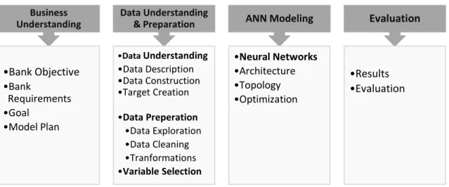
CRISP -DM is the selected method because it has the critical task of business understanding that SEMMA and KDD don’t include. Business understanding helps to ensure the correctness and the maintenance of the results (Chapman et all., 2000). The rest approaches, CIOS, RAMSYS, DMIE and CRISP-DM 2.0 don’t fit our project purpose. In order to adapt the project objective some adjustments were made in content and sequence of CRISP-DM steps. There are 4 phases in the methodology: (1) Business Understanding, (2) Data Understanding and Preparation, (3) Artificial Neural Networks Modeling, (4) Evaluation

Figure 1: Project Methodology

3.1 METHODOLOGY EXPLANATION BUSINESS UNDERSTANDING

The first success step for the predictive model is to understand what the Bank wants to achieve by its use. Identifying the business objective helps to identify (1) critical requirements and (2) create a preliminary solution plan. Misunderstandings of these 2 factors can affect the model´s output and thus, lead to incorrect results. The next step of this phase is to determine certain criteria of what is a successful model for the business. In the current personalized campaign, the bank wants to achieve a high rate of positive answers by contacting less than 50% of the clients. Therefore, the model plan gives an extra variety in response evaluation tools.

Business understanding is not a specific section in this project. The objective of the business became clear at the introduction and the rest factors will be discussed gradually during the report.

Business Understanding •Bank Objective •Bank Requirements •Goal •Model Plan Data Understanding & Preparation •Data Understanding •Data Description •Data Construction •Target Creation •Data Preperation •Data Exploration •Data Cleaning •Tranformations •Variable Selection ANN Modeling •Neural Networks •Architecture •Topology •Optimization Evaluation •Results •Evaluation

(15)

7

DATA UNDERSTANDING AND PREPARATION

The Data Understanding phase starts with the description of the acquired data including, quantity details, row filters and variables explanation. This step is important for getting useful information regarding data and identify potential opportunities for the model. The construction task usually appears in the data preparation phase, but in this project, is part of the data understanding. The extracted dataset includes only from monthly information, and thus, it lucks of historical behavior. Therefore, after analysis and discussion with the business expert, the variables that correlate with customers’ bank mobility are identified and new with largest history are constructed. Last step of this phase is the target creation which includes also the selection of the training DataMart.

The Data Preparation phase involves all the activities need to create the final input dataset. It starts with explanatory analysis, where important statistics measures and graphs are analyzed. The purpose is to read the variables in a more technical way and design a treatment plan. In data cleaning, the results of explanatory analysis are used to manage the inconsistent and problematic attributes and give them a relevant form. Finally, Transformation are applied to boost model performance and then the Input variables are selected.

It must be noticed that data collection and data quality tasks of CRISP-DM are not part of this report. These tasks were others team workshop and they are related with the building of Bank´s Data warehouse.

ARTFICIAL NEURAL NETWORKS MODELING

In this phase, the modeling technique is detailly described. It starts with the basic architecture, where all the neural networks components are presented. This step is important to create a vision for the model and its process. Next, topology describes detailly how the model will treat to the data, in order to get the predicting function. This a critical step for the algorithm performance. Wrong choices here, can make the algorithm slow, more expensive and also unable to find a solution. Last, optimization backpropagation presents how the model will act to improve the solution, or more formal to achieve convergence. Topology and optimization are highly dependent in this type of model. Specifically, the error of the neural network output, is the one will be used to update the model parameters and optimize the solution.

(16)

8

EVALUATION

It is the final phase of the data mining process and a critical step to understand the model´s validity as problem solution. The results got from the algorithm are organized and evaluated in this section. The term organized, refers to the creation of the appropriate metrics and graphs, that needed to evaluate the results. Different business problems, focuses mainly in different evaluation metrics. In the current model, the interest is mainly in the positive responses gained by the deployment of a predictive model. Next, the term evaluation, refers to the comparison of these metrics with (1) standard mathematical criteria and (2) the business goal. Terms such as accuracy, overfitting and gain are discussed in these 2 parts.

(17)

9

4. DATASET UNDERSTANDING AND PREPARATION

Real world data tend to be incomplete, noisy and inconsistent (Han, Pei and Kamber, 2011). Thus, an analysis with this kind of data can lead to misleading and wrong results. Data understanding and preparation are two close loop components for restructuring data and improve model performance.

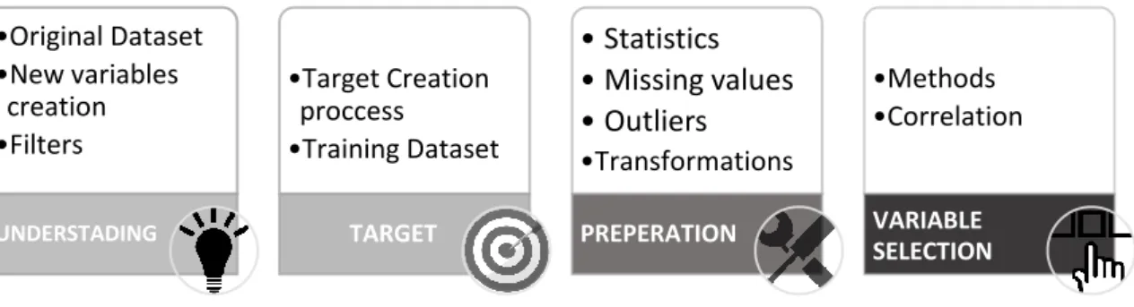
The first part of this section determines the main parts of the dataset and the Target creation procedure. The second part analyzes the data preparation process, including: (1) missing values, (2) outliers and (3) transformations. At the end, the selected variables are defined.

Figure 2: Data Understanding and Preparation Process

The bank data are a high confidential information according the European General Data Protection Regulation (GDPR) (Regulation (EU) 2016/679). Hence, a sample and a summarized explanation of the dataset will be presented in the rest report.

4.1 DATA UNDERSTANDING

4.1.1 DATA DESCRIPTION

The source datasets consist of 12 DataMarts, where each one presents a monthly snapshot of the Data warehouse for the time 30-04-2016 to 31-3-2017. DataMarts consist of 191 original variables and around 1.400.000 clients each. An age filter has applied in the Data Marts to ensure that the clients in the model are adults. The project objective requires to keep only the clients that really interact with the bank in this period. To create accurate models its mandatory to ensure that the clients of the bank are regular and active. Thus, a filter based on customer last movements applied, demanding that the client had at least 1 interaction with the bank the last 4 months. The

•Original Dataset •New variables creation •Filters UNDERSTADING •Target Creation proccess •Training Dataset TARGET • Statistics • Missing values • Outliers •Transformations PREPERATION •Methods •Correlation VARIABLE SELECTION

(18)

10

term interaction refers to a great prism of activities, for a simple call to complicated assets and investments. The number of 4 months is the best choice for minimizing the customer reduction from the filter. The new population is around 1.200.000 clients for each DataMart.

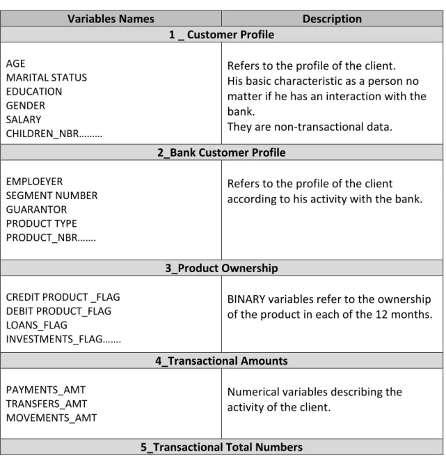
The following table groups the 193 original variables into 6 categories based on their purpose or type. Customer_Profile, Bank_Customer_Profile, Product_Onwership, Transactional_Amounts, Transactional_Total_Numbers and Others. Customer_Profile, and Bank_Customer_Profile describe the client behavior in a more static way. The Product_Onwership are binary variables, which are dedicating the product ownership. The Transactional_Amounts and Transactional_Total_Numbers are describing the exchange activity with the bank. The rest are called “Others”.

Table 2: Original Variables

Variables Names Description

1 _ Customer Profile AGE MARITAL STATUS EDUCATION GENDER SALARY CHILDREN_NBR………

Refers to the profile of the client. His basic characteristic as a person no matter if he has an interaction with the bank.

They are non-transactional data. 2_Bank Customer Profile

EMPLOEYER

SEGMENT NUMBER GUARANTOR PRODUCT TYPE PRODUCT_NBR…….

Refers to the profile of the client according to his activity with the bank.

3_Product Ownership

CREDIT PRODUCT _FLAG DEBIT PRODUCT_FLAG LOANS_FLAG

INVESTMENTS_FLAG…….

BINARY variables refer to the ownership of the product in each of the 12 months.

4_Transactional Amounts

PAYMENTS_AMT TRANSFERS_AMT MOVEMENTS_AMT

Numerical variables describing the activity of the client.

(19)

11 PAYMENTS_NBR

TRANSFERS_NBR CHECKBOOKS_NBR

Total times the activity took place

6_Others EXPENSES_AMT HUNTING_AMT MIN/MAX_ACCOUNT_AMT VOCATION_AMT COMMUNICATION_FLG…

Nor transactional nor profile variables. For the first there is not a straight interaction.

For the second, the velocity of change is high to characterize a client.

4.1.2 DATA CONSTRUCTION

Probably, the most common reason for a model to fail, is that not all the right variables are included in the dataset. For example, the Bank movements are increasing in high seasons, such as Christmas, and decreasing the rest months. Thus, it is reasonable to catch more behavior by adding variables like Averages, Ratios and percentages. Moreover, most of the times a variable fails to fit the model because it misses the variance of another one, where together as total affect the target. For instance, the monthly Car_Expenses maybe affect the monthly Savings, through the previous months Car_Expenses. For this case, variables such as correlations and Ratios based on time are created.

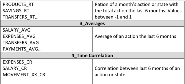
Of course, there are plenty of interactions between variables. However, the purpose of this section is not to identify completely the needs of our model but to enrich the variation of the initial sources. At the end, 103 time oriented variables are created which are grouped in 4 categories. Ratios, Averages, Time_Corellation and Total Percentages the last 6 months. It must be noticed that not all the DataMarts had the appropriate history for this action. Variables are generated for 31-08-2016 to 31-03-2017.The following table gives a brief explanation of its group.

Table 3: Generated Variables

Variables Description

1_Total Percentages PRODUCT_XX_PM

TRANFERS_PM GARNISHMENT_PM…

The Percentage of an action or state the last 6 months.

(20)

12 PRODUCTS_RT

SAVINGS_RT TRANSFERS_RT…

Ration of a month’s action or state with the total action the last 6 months. Values between -1 and 1 3_Averages SALARY_AVG EXPENSES_AVG TRANSFERS_AVG PAYMENTS_AVG…

Average of an action the last 6 months

4_Time Correlation EXPENSES_CR

SALARY_CR

MOVEMENT_XX_CR

Correlation between last 6 months of an action or state

4.1.3 TARGET CREATION

Identify the right target is a critical step in a predictive model. A model can fail if the dependent variable is not representing correctly the customers behavior and the objective of the business.

The first common reason for such cases is not deep comprehension of the business problem. In this case, the client can get unlimited the PRODUCT_XX, but the bank focuses only to the potential new buyers. Thus, a filter showing that he didn’t buy the product before is used. The second main reason is the limited amount of history provided to build the target. Specifically, the frequency in which the customer buys a bank product, it can be weeks to months to years. Therefore, a client can be targeted as buyer even if he bought the product 6 months before. Consequently, almost all the months will be used to construct the target. 10 months as historical data and 2 months as extra score sets for checking future performance.

The final target is a binary variable where if the client bought the product in the training month and never before, then is a buyer. The corresponding DataMart is 31 January 2017 and the amount is 0,13 %. The training dataset it consists of 193 variables based on January 2017 plus the derived variables relevant to this month. It has 1.202.689 clients. It made clear to the business that this value is very small to ensure that the model will give accurate results, but the business expert insisted to get scores.

Figure 3: SAS code for Target Creation

PRODUCT_XX_T = IF SUM (PRODUCT_XX_FLAGm1…PRODUCT_XX_FLAGm9) = 0 AND PRODUCT_XX_FLAGm10= 1

(21)

13

The following figure shows the percentage of Target positives in each month and the model time window. The left skewed side is the history period. The right skewed side are the extra score months.

Figure 4: Target percentage per month and model Time window

4.2 DATA PREPERATION 4.2.1 EXPLANATORY ANALYSIS

After understanding the source data, the second step is to get some insights regarding their shape and their values. Data explanatory analysis will provide fundamental statistics, helping to identify potential data treatments or variables rejections. SAS Guide and Miner are combined in this part to give 360◦ view of the dataset.

The results of the explanatory analysis are divided in 3 main groups: (1) Statistic measures, (2) frequency charts - Graphs and (3) frequency table of categorical variables.

(22)

14

Figure 5: Explanatory Analysis

The first Category characterizes the data based on measures of central tendency and dispersion. It gives a great view of the data, by identifying for each variable basic statistic measures, the level of dispersion, extreme rows and amount of missing.

The second group, Frequency Graphs and Charts, it characterizes data at a glance. They fulfill Statistic Measures and create a solid picture of the dataset. Frequency Graphs are used for numerical variables and they show the frequencies of variable observations based on binning. Charts are doing the same but for categorical variables. Their main advantage is, that they provide information for outliers by showing the distance of each observation from the variables global concentration.

Lastly, the frequency table for categorical variables it gives the 10 most frequent district values per categorical variable. It extends the frequency chart by presenting a numerical view of the counts.

4.2.2 DATA CLEANING

MISSING VALUES

Missing data in the training data set can reduce the power of a model by introducing incorrect behavior in the model. Data can luck for several reasons such as be Missing at Random (MAR), Completely at Random (CMAR) and not Random (NMAR) (Little and Rubin,2002).

Missing Random: the missing value it depends for other observed values Completely Random: missing values are independent for the observed values Not Random: the distribution of the Missing depends on the missing values.

•Mean, Median, Mode •Missings •Standard Deviation •Min , Max G ra p h s an d C h ar t •Histogram frequency Graph •Frequency Chart N o mi n al C o u n ts •Frequency table of categorical variables Sta ti sti c Me as u re s

(23)

15

Several ways are recommended by literature to treat missing values. The most common are:

Delete: delete the values that are missing. It’s not recommended because it reduces the sample and thus the behavior.

Replace: replace the value with mean, median or mode of the variable. Sometimes the results are much different than the once if the values were known.

Predict: predict missing values by using as predictors the other variables. Is good when the missing are NMAR and there is actual relation between the variables.

KNN: K- Nearest Neighbor. The missing values of an attribute are replaced based on similarity with other attributes. Sensitive to the choice of k - number of attributes. User Defined: assign the missing values based on experience and dataset knowledge.

In this case study 2 methods applied. (1) The variables that had more than 20% of missing are excluded. With this percentage, it is risky to replace values and being sure that not wrong behavior is introduced to the model. (2) For the rest values, the user defined method is used. The bank databases are mostly accurate and a guideline for the missing values exists. Usually a missing value means that there was not this kind of action, thus, it takes the value 0.

OUTLIERS

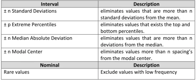
Outliers´ detection and treatment is a very important part of any modeling exercise. A failure to detect them can have a serious impact on the model validity. According to (Tiwari, Mehta, Jain, Tiwari and Kanda, 2007) outliers are a set of observations whose values deviate from the expected range. The problem with outliers is that they can increase the error variance, affect the significant tests and lead to incorrect conclusions. There are several opinions regarding outliers’ treatments. (Cousineau and Chartier, 2010) mentioned that if outliers follow a distribution close to normal, then the influence of low and high outliers on the mean is more likely to neutralized. Usually this brings a type -II error. In such conditions is better to use z-score detection methods like standard deviation and extreme percentiles to remove them. If the variable doesn’t follow normality, then the skewness can cover outliers. In this case, it is better first to apply a nonlinear transformation in the dataset and then move to the detection. (Tiwari, Mehta, Jain, Tiwari and Kanda,2007) focused on capping and flooring methods. In these methods, the value that exceeds the 99th_{, 1}st_{percentile or is N times far for the mean, it} is capped or floored in another value closer to it. Furthermore, the outliers´ treatment can be really difficult when there are many variables in the dataset. With high

(24)

16

dimensionality, all the data values are far from each other and it’s hard to identify the extremes. (Filzmoser,2004), supports the mehalanabolis distance method, where for its point the distance for the average its calculated, considering also the covariance matrix. The main benefit is that distinguishes the extremes of a distribution and the actual outliers. Finally, there are researchers support that outliers are extreme behaviors, and thus, they must remain in the sample.

The most common outlier’s treatments are:

Table 4: Common Outlier Treatments

Interval Description

± n Standard Deviations eliminates values that are more than n standard deviations from the mean. ± p Extreme Percentiles eliminates values that exists the top and

bottom percentiles.

± n Median Absolute Deviation eliminates values that are more than n deviations from the median.

± n Modal Center eliminates values more than n spacing’s

from the modal center.

Nominal Description

Rare values Exclude values with low frequency

After discussion with the business expert, all the extreme buyers are important and their values has a meaning for the bank. Outliers didn’t delete.

4.2.3 DATASET TRANSFORMATIONS

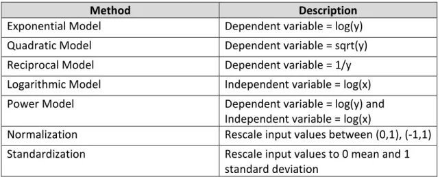
Sometimes, the observations of the variables are not immediately suitable for the analysis. Instead, they need to be transformed to meet the algorithm requirements. These requirements can be statistical assumptions or choices to boost the model performance. For example, in Ordinary Least Square regression the parametric tests can be affected if the residuals don’t follow normality. In other cases, the algorithm performance can be decreased just because the variables don’t have the appropriate numeric scale. Specifically, in Neural Networks is hard to minimize the error if the values are very far from each other.

(25)

17 The most common transformations are:

Table 5: Common Transformations

Method Description

Exponential Model Dependent variable = log(y)

Quadratic Model Dependent variable = sqrt(y)

Reciprocal Model Dependent variable = 1/y

Logarithmic Model Independent variable = log(x)

Power Model Dependent variable = log(y) and

Independent variable = log(x)

Normalization Rescale input values between (0,1), (-1,1)

Standardization Rescale input values to 0 mean and 1

standard deviation

In this project, the input variables transformed by adjusting the values using standardization. Literature recommend this for ANNs.

4.3 VARIABLE SELECTION

Choosing the correct features, it is core in predictive modeling. Variable selection improves data understanding, reduces storage requirements, decreases training time and defies the high dimensionality (Guyon and Elisseeff,2003). There are two main methods for selecting the variables: (1) Filter methods and (2) Wrapper methods. Filter Methods: measure the relevance of a variables´ subset. The selection procedure is independent of the learning algorithm and is generally a pre-processing step (Guyon and Elisseeff,2003). They are robust to overfitting and the selected variables are easy to interpret. Filter methods use a statistical measure to assign a score in the variables and then delete the most irrelevant. Chi square and correlation coefficient are some of them. Wrapper Methods: measure the usefulness of a variables´ subset.They are prone to overfitting but relevant to find effective variables. Here, the subset selection is dependent on the learning algorithm. A predictive model is used to evaluate many variables combinations and create a subset based on accuracy. The final variables are those who return better results. The Forward selection and Backward are well known.

(26)

18

Table 6: Variable Selection Common Strategies Method

Filter Description

Chi square

(categorical variables)

Chi square test applied to check the independency for the target.

Information Gain Information Gain (Entropy, Gini) is calculated for all inputs. Features with highest values are selected. Weight of Evidence (WoE) Calculates information value (IV) of each input and

selects those with highest IV.

Correlation Coefficient Variables with Correlation> 80% are excluded Wrapper

Forward Selection Start with 0 variables. Keep adding features to the model until the model stop to improve

Backward Elimination Start with all features. Remove in its iteration the least significant until no improvement

Stepwise considers adding and deleting predictors at each step

of the process

In this project, both filtered and wrappers methods are used. Filter methods are used to select variables that affect the target based on the business insight. Explanatory variables need to tell a story for the output, otherwise the results may be based on randomness and be inappropriate for future use. First, Chi square test is used to rank the categorical variables and WoE to rank the numeric variables. Then the high correlated variables are excluded using Pearson’s correlation coefficient. At the end, a wrapper method is applied to confirm 2 ideas: (1) The appropriate number of inputs and (2) which variables strongly affect accuracy. The selected wrapper method is stepwise regression.

(27)

19

Table 7: Input Variables

Input Variables Type Description

Credit_Card_Flag_S binary Ownership of Credit Card

Life_Insurance_Flag_S binary Ownership of life Insurance

Prepaid_Card_Flag_S binary Ownership of Prepaid Card

Term_Deposit_Account_Flag_S binary Ownership of Term deposit

Debit_Card_Flag_S binary Ownership of Debit Card

Renew_Saving_Flag_S binary Flag of renew the Savings account Contact_Less_Card_Flag_S binary Ownership of Contact Less Card Nbr_Movements_4m_S numeric Number of activities last 4 months Amount_Credit_Card_Approv_A numeric Average amount of credit card limit

Nbr_Products_S numeric Number of products owns

Entity_Tenure_S numeric Amount in days of being client

Personal_Credit_Flag_PF numeric % of months with Personal Credit Investiments_Products_Flag_PF numeric % of months with Investment products

(28)

20

5. ARTIFICIAL NEURAL NETWORKS MODELING

The first part of this section describes all the basic components need for building an artificial neural network. The second part explains the network’s structure, including interconnections and networks implementation. Finally, the third part of this section presents the optimization technique and its parameters choices.

Figure 6: ANN Model Process

5.1 BASIC ARCHITECTURE

There are many different ANN models but each model can be precisely specified by the following 10 major aspects based on (Rumelhart, Hinton and Williams, 1986):

(1) Set of processing units/neurons: neurons receive one or more inputs from another sources or neurons. Neural Network combines these inputs, performs a generally nonlinear operation on the result, and then compute an output value. Three types of neurons:

Input: receives their input from the data source. Output: send signals out of the neural network

Hidden: their input and output signals are inside the network.

(2) Layers: neurons with same characteristic can be grouped together and arranged on layers. Thus, there is input layer, output layer and n hidden layers.

(3) Synapsis/Topology: specifies if and how a neuron is connected to the other neurons in the network. A real number called synaptic weight (𝑤𝑖(𝑡)) is used to define the strength of the connection. Weight, determines the amount of effect that the first

•What are Network's: •Neurons •Weights •Functions •Learning rule BASIC ARCHITECTURE •Structure: •Interconnections •Implementation TOPOLOGY •Which: •Algorithm •Learning rate •Momentum OPTIMIZATION

(29)

21

neuron has to the upcoming neuron. The pattern of connectivity for a whole network with N units can be represented by the weight matrix [W].

(4) Activation State: Network processes information through neurons (Kriesel, 2005). This information is numerically expressed as activation value. The pattern of activation captures what the system is representing at any time t, and called activation state. The activation value of a 𝑛𝑒𝑢𝑟𝑜𝑛𝑖 the time t is 𝑎𝑖(𝑡). The values can be discrete, continues or with boundaries.

(5) Output function: Neurons interact by sending output signals. The output function 𝑓𝑖(𝑎𝑖(𝑡)) uses as argument the activation value 𝑎𝑖(𝑡) to calculate the output value of the neuron denoted by 𝑜𝑖(𝑡). Usually, the function is the identity.

𝑜_𝑖(𝑡)= 𝑓(𝑎𝑖(𝑡))=𝑎𝑖(𝑡)

(6) Propagation/Combination function: a neuron can have several inputs. Propagation function defines how the network will combines the weight matrix and output values 𝑜𝑖(𝑡) to produce the input for another neuron, called net input (𝑛𝑒𝑡𝑖(𝑡)). Usually this relationship is additive.

𝑛𝑒𝑡𝑖=∑( 𝑜𝑖(𝑡) ∗ 𝑤𝑖,𝑗(𝑡) )

(7) Threshold /bias node: a constant typically 1 or -1, which used also to calculate the net input of the neuron. Is equivalent to intercept in a regression model and is treated as a connection weight.

(8) Activation function: defines how the network will treat to the net input and the current activation value, to produce the next step activation state 𝑎(t+1). Well-known functions are the linear, the threshold, sigmoid, tan and log sigmoid.

𝑎_𝑖(𝑡 + 1) = 𝑓(𝑎𝑖(𝑡), 𝑛𝑒𝑡𝑖(𝑡))

(9) External environment: provides input sources to the network and receives the outputs. Interacts with the network during the supervised leaning phase to evaluate the results.

(10) Learning Rule: is a formula based on the learning type to adjust the weight matrix [W] and the bias term. These adjustments change the output behavior and improve network performance.

(30)

22

The following figure shows the process of a neuron, that receives 2 outputs from other neurons as inputs. These are combined with synaptic weights and bias in a simple additive operator to extract the net input. A sigmoid activation function calculates the next activation value. Finally, the output of the neuron is identical to the current activation value.

Figure 7: General Neuron Process

5.2 TOPOLOGY

Interconnection between neurons can be done in numerous ways, leading to several topologies. These can be divided into two basic categories. Feedforward and Feedback (or recurrent) neural networks (Krenker, Bester and Kos,2011).

Feedforward: The information flows in one direction, from input to output. Neurons send their outputs to neurons, from which they don’t receive an input directly or indirectly. Simply, there are no feedback loops. Furthermore, feedforwards networks implement a static mapping between input and output space. Specifically, the synaptic weights are fixed after every training, meaning that the state of a neuron is determined by the input and output pattern and not by the initial and past states of the neuron. A typical application of feedforward networks is pattern recognition or Classification. The most common feedforward neural network is the strictly forward where neurons are connected only to the neurons situated in the next consecutive layer.

(31)

23

Feedback: The information flows from both directions, input to output and output to input. There is at least one feedback loop. This structure of feedback networks makes the weights adjustable and leads to a dynamic mapping between input and output space. Here, the state of neuron depends not only of the current input signal, but also from the previous states of a neuron. A typical application of feedback networks is Time Series, Natural Language Processing (NLP) and Machine translation. The most common feedback neural network is the fully recurrent where every neuron is directly connected with all neuron in any direction.

The following figure shows an example of a feedforward (a) and a feedback (b) network.

Figure 8: Feedforward and Feedback Networks

Both methods have advantages and disadvantages. Feedforward networks are easily to build but they cannot deal well with data that were never learned in the training phase. Also, if the data set is very large the speed of convergence can be very slow. On the other hand, feedback methods they effectively decrease the training time but they have an important disadvantage. The nonlinear nature of neuron activation output and the adjusted synaptic weights can affect the network stability (Chiang, Chang, L. and Chang, F., 2003).

In terms of business objective, the effect of unstable network is unreal unbalances in the customer behavior, which can lead to failure the personalized campaign. Simply, the probabilities of score DataMarts should only differentiate because of changes in customer behavior.

Thus, the selected method is the feed-forward. The most well-known feed-forward models are Perceptron, Multilayer Perceptron and Radial basis function.

(32)

24

Perceptron: The single-layer perceptron model consists of one layer of input neurons and one layer of output neurons. There are no hidden layers and therefore, there is only one layer of modifiable weights.Perceptron can only model linearly separable classes. Multilayer Perceptron(MLP): has one or more hidden layers between the input and output layers. The existence of hidden layers, specifically their activation function, allows MLP to solve nonlinear problems. The propagation function of the neuron is a weighted sun of the input values plus the bias term. The output value of the neuron is identical to its activation state where the output of the network is a weighted sum of all the activation values. Multilayer Perceptron can solve more complicated problems such as function approximation, pattern classification and optimization (Silva et al., 2017). Radial Basis Function (RBF): has only one hidden layer between input and output layers. It works also well with advanced problems like the MLP does. Here the propagation function it calculates the distance (usually Euclidian) from the neuron center. The neuron center can be a random vector of the train set or a calculated cluster mean. There is no weighted connection between input and hidden layer. The activation function is a radial basis function (usually Gaussian), that gives a value 1 if the input is exactly same to the center, or 0 otherwise. The output is the weighted sum of the activation values from every RBF neuron.

The applied model is the feed forward multilayer Perceptron as it is the most applicable in business environments (Popescu et al., 2009).

5.3 OPTIMIZATION - BACKPROPAGATION

To optimize the performance of a supervised feedforward ANN, the predicted values must be as close as possible to the desired value. Backpropagation algorithm is the most popular method because is conceptually simple, computationally efficient and works most of the times (Lecun et al. ,1998). The BP algorithm uses the same principle as the Delta Rule, minimize the sum of the squares of the output error, averaged over the training set. It is also called the Generalized Delta Rule (Nascimento, 1994). The advantages of Backpropagation are, the small number of parameters need to be defined, the easy algorithm implementation, and its ability to solve complex nonlinear problems. It’s a universal approximator, meaning that for every possible input x, the value f(x) can be approximated by a backpropagation neural network (Priddy and Keller,2005). It belongs to First order optimization methods, using only the first order error derivatives to adjust the parameters and minimize the loss function (Madani, 2016). Specifically, it adapts the Gradient Descent algorithm. The process of the neural network is to update at each iteration the adapted parameters (synaptic weights and bias) until convergence.

(33)

25

(𝑤𝑖+1= 𝑤𝑖 − 𝑎 ∗ 𝑑(𝑒𝑟𝑟𝑜𝑟) + 𝜇 ∗ Δw(𝑡 − 1)

The formula above shows a weight updating of backpropagation algorithm where: (- 𝒅(𝒆𝒓𝒓𝒐𝒓)): is the partial gradient of the error function with respect to parameters (w and bias). The minus is used because the parameters must move opposite of the gradient. Specifically, to the decreasing direction of the error function (minimum). (𝒂): it is the learning rate parameter. It defines the proportion of the error will be used for weight updating. Large values of the learning rate create many fluctuations in the error reduction, preventing to find the minimum point. Small values make the convergence very slow.

𝝁 ∗ 𝚫𝐰(𝒕 − 𝟏): it is the momentum term. Momentum adds the influence of the last weight change on the current weight change. This term increases the speed of convergence, by helping parameters move to the direction of the global minimum and overcome local minimums (Burney, Jilani and Ardil, 2007).

The following table (Sarle,1999) from SaS Institute, summarizes the performance of the backpropagation based on different values of learning rate and momentum. The first column applied to a “good” dataset and shows the time need to be achieved a minimum error. The second column, shows the error in a” poor” dataset after 1000 iterations. The variables are normalized.

Table 8: Error of different Learning Rate and Momentum values

Good Dataset MSE=0.001 Poor Dataset >1000 Iterations Momentum = 0 LR=0.1 519 0.0147 LR=0.2 259 0.0356 LR=0.5 51 0.8302 LR=1 >1000 18 Momentum = 0.9 LR=0.1 93 0.0058 LR=0.2 86 0.0029 LR=0.5 96 0.0002 LR=1 173 1.55

It is obvious that the use of momentum speeds up convergence, so, it is used. Regarding learning rate, small values make the algorithm slower but large values make it unable to find the minimum. Both the values of momentum and learning rate are decided after trials, to fit better the current data shape.

The table below summarizes the neural network structure, including topology´s and optimization´s final parameters and functions. It must be noticed that the number of neurons and hidden layers is based on the trial and error method.

(34)

26

Table 9: final Artificial Neural Network Parameters

Topology

Interconnections Feedforward

Model Multilayer Perceptron

Number of hidden neurons 7

Number of hidden layers 1

Number of output neurons 1

Bias Yes

Output function Equal to activation

Hidden layer Activation function Tanh Hidden layer Combination function Linear

Target layer Activation function Logistic sigmoid (probabilities) Target layer Combination function Linear

Direct Connections No

Optimization

Algorithm Gradient Descent Backpropagation

Error model _{𝑀𝑆𝐸(𝑡) =} 1 𝑁∑ ( 𝑁 1 𝑦̂(𝑡) − 𝑦𝑖), average error Learning rate 0.1 Momentum 0.2 Iterations Max 100

(35)

27

Figure 9: Model Architecture

The above figure shows the final architecture of the neural network. 13 input neurons are used, equal to the number of variables. It’s a strictly feedforward neural network with one output neuron. The binary classification problem, requires just one output neuron for a solution. It predicts the class 1 for customers with probability to buy greater than 0.5 and 0 otherwise. The cut-off point can differentiate in order to allocate the output class.

(36)

28

6. EVALUATION

Evaluating the performance of a model is one of the core stages in the data science process. It indicates how successful were the predictions of a dataset based on a trained model. According to (Shiffrin, Lee and Kim, 2008), a good model must make accurate predictions for the data and for alternative data circumstances. It must provide insights for the data that are not directly clear, generate opportunities for further studies and clarifies whether theory fails or not. In order to boost the performance of the algorithm an under-sampling (SAS Miner default) 18% of Target is used. The new dataset has 26968 observations, where 5920 remain the target class. The dataset is split then, into training and test set using the rule of thumb proportion 70% and 30%. This section first evaluates the model performance based on comparison between seen and unseen data. Overfitting and correctness are discussed in this phase. Then, the rest two DataMarts are scored, providing information for future performance and fulfilling the analysis regarding generalization ability.

6.1 RESULTS AND EVALUATION

The evaluation phase starts mainly by categorizing the predicted observations in 4 groups with respect to their true values (Sokolova and Lapalme, 2008).

True Positives: observation classified as buyer whose true class is buyer False Positive: observation classified as buyer whose true class in not buyer True Negative: observation classified as not buyer whose true class is not buyer False Negative: observation classified as not buyer whose true class is buyer

These 4 groups are arranged into a 2 x 2 matrix, called confusion matrix, which provides information regarding the total model performance. The upper left side of the matrix shows the sum of true positives and the lower right side the sum of true negatives. The sums of the wrong predictions FP and FN are in lower left and upper right corners.

•Confusion matrix •ROC curve •Gain chart •Lift chart •Maintenance EVALUATION

(37)

29

Figure 10: Confusion Matrices of Training and Test sets

A number of metrics and graphs useful for the analysis can be arranged from the confusion matrix. The following figure summarizes the most common.

Figure 11: Evaluation Metrics Performance Metrics

Train set Test set

Accuracy (TP + TN) / (TP + TN + FP + FN) % of correct classified

Error rate 1 – accuracy % of wrong classified

Precision TP / (TP + FP) % of predicted buyers, which are actual

buyers

Recall/Sensitivity TP / (TP + FN) % of actual buyers classified as buyers

Specificity TN / (TN + FP) % of predicted non-buyers, which are actual

non-buyers

True Positive Rate TP / (TP + FN) Sensitivity

False Positive Rate 1 - (TN / (TN + FP)) % of actual non-buyers classified as buyers

The accuracy gives a first view of the overall model effectiveness, by showing the total % of correct classifications. In this study 87.66 % of known data and 87.69% of unknown data are correct classified. The error rate is quite small with a percentage of 12%. These numbers are satisfied, but only accuracy cannot guarantee the quality of a model. A very common phenomenon in imbalanced datasets is the model to assign all the observations in the highest frequency class and coming up with also high accuracy value. Specificity and sensitivity are good metrics to identify this case. With values, around 93% and 60% respectively it is shown that the ability of the model to identify TP is not so satisfied. However, in probability estimation models the cut-off level plays an important role in the output results. In this case, it is assumed that a client is a buyer if his probability is higher or equal to 0.5. In reality, this threshold is not known and values of sensitivity and specificity can change a lot with small adjustments to these values (Fan, Upadhye and Worster, 2006). The purpose of this study is to identify probabilities for

(38)

30

outreaching clients and not classify them. Thus, the main evaluation tools will be the ROC curve and Gain, Lift charts. For the previous metrics, it is important to keep that the values for both training and test set vary together giving the confident that model does not overfit the data.

Figure 12: Evaluation Results Train and Test sets Performance Metrics

Train set Test set

Accuracy 87.66% 87.7%

Error rate 12.34% 12.32%

Precision 68.1% 67.7%

Recall/Sensitivity 59.1% 60.1%

Specificity 93.9% 93.7%

ROC curves are the most popular technique to visualize the performance of a binary classifier. They are insensitive to class distributions and do not account imbalance in the data sets (Provost and Fawcett, 1996). ROC curve is a two-dimensional graph of True positive rate (y-axis) against False positive rate (x-axis) that quantifies the performance of a classifier in reference to all possible probabilities thresholds. Specifically,allows to see, how sensitivity and specificity vary as the threshold varies. The lower left point of the plot (0,0) demonstrates a strategy of always predicted non-buyer. Neither TP nor FP exists. The upper right corner (1,1) corresponds to a model that classifies all observations as buyers. In this cases FPR and TPR getting their maximum values. The upper left corner (0,1) provides the perfect classification, where sensitivity gets a maximum value of 1 and FPR a minimum of 0. This point corresponds to a threshold that discriminates buyer with non-buyers 100% correct. The hypothetical line y=x represents the strategy of random guessing. AUC, the area under the curve, quantifies the model discrimination power. The maximum value is 1, representing the perfect classifier at point (0,1). Because it´s not realistic to get a classifier worse than random guessing the minimum value assumed to be the 0.5. AUC has an important statistical characteristic. It represents the probability that a classifier will rank a randomly chosen positive instance higher than a randomly chosen negative instance (Fawcett, 2003). Therefore, the AUC evaluates how well a classifier ranks the predicted observations.

(39)

31

Figure 13: ROC curves Train and Test sets

The above figure shows the ROC curves generated by the model for both train and test data. The sharp trade – off between FPR and TPR shows at a glance the existence of a good classifier. The long distance for the random guessing line guarantees that the model performs much better that an arbitrary classification choice. The AUC for training and test data is 0,9008 and 0,9003 respectively. According to the literature it is an excellent classifier, where the threshold is AUC >0,90. It indicates that 90% of the times, a random selection of the buyers group will have a score greater than a random selection of the non-buyers group (Dougherty, 2009). Therefore, no matter that ROC curve is not affected by the probabilities calibration (Mandrekar, 2010), the AUC value gives confidence regarding the correctness of the extracted probabilities. Technically, it proves that the fitness function generated by the neural network is able to classify well the clients under the right choice of a cut- off level. Finally, both train and test set ROC-curves show the same performance, fulfilling the finding regarding no overfitting.

Cumulative Gain or Response curve it is closely related to the ROC curve but it more intuitive (Provost and Fawcett, 2013). In targeted campaigns, response curve it is used to provide information regarding the effectiveness of the model to cost decreasing (Jaffery and Liu, 2009). Technically, the extracted probabilities are sorted from highest to smallest, creating a ranked population scale. Then the percentage of positives correctly classified is plotted on y-axis as a function of the percentage of the population targeted x-axis. Here also the diagonal line x=y represents the random performance. Contrary to the Roc curves, gain charts and lift charts next, have an important assumption. They assume that the test set has exactly the same target class priors as the

(40)

32

population to which the model will be applied (Provost and Fawcett, 2013). Practically, when the train data undersampled or oversampled to fix the balance, the numerical results of the graphs will be different than those with the actual population. Thus, to get realistic results the whole dataset is scored by the trained model, and these results are used to generate the next graphs.

Figure 14: Comulative % Response Curve

The above figure provides the cumulative % Response curve for the whole population of the training month. According to the graph around 70% of the potential buyers can be achieved by contacting the first 10% of the ranked population. Likewise, the top 25% of the population would contain approximately 90% of the positive cases. The random performance line at the same points can only identify the 10% and 25% respectively. In terms of profit, the application of the model will reduce the campaign´s cost at least 50%.

The Cumulative Lift curve measures the model effectiveness by comparing the predictive results against the random performance. It provides the same results as the response curve, but in a more numerical way. Basically, it is the value of the cumulative response curve divided by the random performance line. Here, the diagonal line y=x of response and Roc curve, becomes a horizontal y=1 in this plot. The figure below shows the lift curves of the whole dataset. At the top 5% of the population the model performs 11 times better than random selection. Additionally, by contacting the top 10% of the ranked population the predictive model will reach around 7 times more responders.

0% 20% 40% 60% 80% 100% 0 10 20 30 40 50 60 70 80 90 100 Percentil Capture Baseline

(41)

33

Figure 15: Cumulative Lift curve

Score 2 DataMarts is the last evaluation step decided by the business expert. In next phases, the created model will put into production and new data will be scored at the end of each month. A strategic plan, including contact campaigns and individual offers will be then applied to the ranked population to improve profits. Because the model performance decreased over time, it makes sense to evaluate the model also in terms of maintenance. Thus, the next two months February and March are scored, and their cumulative Gain and Lift curves are compared with the train results. The base rate in the 3 datasets is 0,13% and the total number of observations around 1.200.000 respectively. This balance is the one that allows the comparison of the plots, as they are dependent of classes amounts (Provost and Fawcett, 2013). For functional reasons, the results of the curves are summarized on tables.

Table 10:Cumulative % Gain and Lift of score DataMarts per percentile

Cumulative %Gain Cumulative Lift

Percentile Train Set Score set 1 Score set 2 Train Set Score set 1 Score set 2

10 72,18% 72,22% 72,20% 7,217 7,221 7,219 20 87,50% 87,11% 87,25% 4,374 4,355 4,362 30 93,48% 93,01% 93,22% 3,115 3,100 3,107 40 95,71% 95,64% 95,65% 2,392 2,390 2,391 50 97,65% 97,47% 97,42% 1,953 1,949 1,948 60 98,58% 98,43% 98,58% 1,643 1,640 1,642 70 99,29% 99,17% 99,17% 1,418 1,416 1,416 80 99,71% 99,72% 99,75% 1,246 1,246 1,246 90 99,90% 99,93% 99,93% 1,109 1,110 1,110 100 100,00% 100,00% 100,00% 1 1 1 0 5 10 15 20 25 0 10 20 30 40 50 60 70 80 90 100 Percentil Lift Baseline

(42)

34

The above table summarizes the cumulative % response and lift values for the 3 Datasets. It is obvious that the model performance in the future datasets is almost identical to the training data. This does not give certainty for the future validity, but it gives confident that the performance reduction velocity will be slow.

All the evaluation metrics used in this section prove that the model performs well. It has good discrimination ability, high response rate and potential good future performance.