A new bone tissue remodeling algorithm combining mechanical stimuli with cellular dynamics

Faculdade de Engenharia da Universidade do Porto

A new bone tissue remodeling algorithm

combining mechanical stimuli with cellular

dynamics

Madalena Macedo Alves Peyroteo Gomes

Dissertation carried out under the

Integrated Master in Bioengineering

Biomedical Engineering

Supervisor: Professor Jorge Américo Oliveira Pinto Belinha

Co-Supervisor: Professor Renato Manuel Natal Jorge

ii

iii

Abstract

For decades, bone has been the subject of study of many researchers, due to its capacity to continually renew itself. Nowadays, understanding the basic biology of bone remodeling has become critical and very relevant. This because, having a very thorough knowledge about the normal functioning of the bone, allows more easily the construction of the bridge that permits to discover and describe the pathogenesis of various disorders of bone remodeling. For instance, these disorders can be renal osteodystrophy, Paget’s disease, osteopetrosis, and osteoporosis that affects over 200 million people worldwide [1].

Therefore, this master thesis aims to create a new spatiotemporal model that can replicate the biomechanical and biochemical processes involved in bone remodeling in a healthy state. In order to accomplish it, the agenda was divided in three different stages. First, a mechanical model combining meshless methods with a bone tissue remodeling algorithm was built and tested, based on the model proposed by Belinha [2]. By seeking the minimization of the strain energy density (SED) variable with respect to the bone apparent density, results were able to reproduce the trabecular morphology of bone. The solutions were obtained using three different numerical methods, namely the Finite Element Method (FEM), the Radial Point Interpolation Method (RPIM) and the Natural Neighbor Radial Point Interpolation Method (NNRPIM), using for the first time the RPIM in bone remodeling simulations.

Then, based on the biological model proposed by Ayati [3], a new spatiotemporal model of the cellular response observed during a single cycle of bone remodeling was created. Through him, this phenomenon was simulated for the first time in 2D, obtaining accurate results capable to describe the dynamics of bone cells.

After the validation of these two models, the mechanobiological model was idealized and tested. Using an experimental law that relates the levels of effective stress and the cell density of osteoblasts, results show the growth of bone according to the applied loads. However, further improvements have to be done in this model.

To conclude, with this work, new analysis in 2D were performed, with interesting and encouraging outcomes. The results obtained support the data existent in the literature, validating the models created and the possibility to test them in disease states. Ultimately, these in silico models will allow the development of novel therapies for bone remodeling disorders.

v

Resumo

Ao longo de décadas, vários investigadores têm dedicado o seu trabalho a estudar o osso, devido à sua capacidade de renovação contínua. Atualmente, o estudo e compreensão do fenómeno de remodelação óssea é cada vez mais importante e relevante. Isto porque, o conhecimento aprofundado acerca do funcionamento normal do osso facilita a construção da ponte que permite a descoberta da patogénese de vários distúrbios relacionados com a remodelação óssea. De entre estes distúrbios, estão incluídos a osteodistrofia renal, a doença de Paget, a osteopetrose e a osteoporose, que afeta mais de 200 milhões de pessoas em todo o Mundo [1]

Assim, o objetivo desta tese de mestrado é a criação de um modelo espácio-temporal capaz de replicar os processos biomecânicos e bioquímicos que ocorrem durante a remodelação óssea numa situação saudável. Para isso, o plano de trabalhos foi dividido em três componentes diferentes. Inicialmente, foi criado e testado um modelo mecânico, que combina um algoritmo de remodelação de tecido ósseo e métodos sem malha, baseado no modelo proposto por Belinha [2]. O modelo consiste na minimização da densidade de energia de deformação em relação à densidade óssea aparente e os resultados foram capazes de reproduzir a morfologia trabecular existente no osso. As soluções foram obtidas usando três métodos numéricos diferentes, nomeadamente o Método dos Elementos Finitos, o Método da Interpolação Radial e o Método da Interpolação Radial dos Vizinhos Naturais, sendo que foi a primeira vez que o Método da Interpolação Radial foi testado em simulações de remodelação óssea.

De seguida, foi criado um novo modelo espácio-temporal da resposta celular observada durante um ciclo de remodelação óssea, a partir do modelo de Ayati [3]. Este fenómeno foi simulado pela primeira vez em 2D, tendo-se obtido resultados capazes de descrever com muita acurácia o comportamento das células ósseas.

Após a validação destes dois modelos, o modelo mecanobiológico foi idealizado e testado. Recorrendo a uma lei experimental que relaciona os níveis de tensão efetiva e a densidade celular de osteoblastos, os resultados mostraram o crescimento ósseo de acordo com o desenho das cargas. No entanto, existem vários aspetos a melhorar neste modelo.

Concluindo, através deste trabalho, novas análises em 2D foram executadas, produzindo resultados interessantes e promissores. Estes resultados estão de acordo com a informação existente na literatura, validando os modelos criados e a possibilidade de os testar em estados de doença. No futuro, o objetivo ideal seria usar estes modelos in silico no desenvolvimento de novas terapias para doenças relacionadas com desequilíbrios durante a remodelação óssea.

vii

Acknowledgments

Estes últimos 5 meses foram repletos de novos desafios, que teriam sido impossíveis de ultrapassar sem a ajuda do meu orientador, o Professor Jorge Belinha. Por isso, queria começar por agradecer profundamente pelo acompanhamento e dedicação constantes. O projeto era ambicioso e trabalhoso, não fosse a sua visão pragmática e um entusiasmo que me contagiava à medida que cada objetivo era cumprido. Gostava também de agradecer ao meu co-orientador, o Professor Renato Natal, pela sua disponibilidade e acompanhamento.

Mas, como para chegar aqui passaram 5 anos, queria agradecer também à minha família e aos meus amigos. À minha mãe pelos beijos, à minha avó pelos abraços, ao meu pai pelo mimo e ao meu avô pelos sorrisos. Às minhas irmãs Mariana por enlouquecer quando eu preciso e Inês pela loucura constante.

Queria agradecer também ao meu eterno Bando, aqueles amigos para sempre e a todas as amizades que fiz durante a Faculdade. Em especial, à Ana/Minguante/Nobe/Mingas/Berlim. Tantos nomes e todos com o mesmo significado: companhia inseparável.

Por fim, queria agradecer à Tuna Feminina de Engenharia, por me ter embalado durante estes 5 anos e mostrado que quando bem aproveitado, temos tempo para tudo. É um orgulho pertencer a este grupo e passar por tantas aventuras sempre na melhor companhia.

ix

Funding

The author truly acknowledge the logistic conditions provided by Ministério da Educação e Ciência– Fundação para a Ciência e a Tecnologia (Portugal), under project funding UID/EMS/50022/2013 (funding provided by the inter-institutional projects from LAETA) and project NORTE-01-0145-FEDER-000022 - SciTech - Science and Technology for Competitive and Sustainable Industries, cofinanced by Programa Operacional Regional do Norte (NORTE2020), through Fundo Europeu de Desenvolvimento Regional (FEDER).

Additionally, the author truly acknowledge the work conditions provided by the department of Mechanical Engineering from FEUP and INEGI.

xi

“This is where it all begins. Everything starts here, today”

xiii

Contents

Abstract ... iii

Resumo ... v

Acknowledgments ... vii

Funding ... ix

Contents ... xiii

List of Figures ... xv

List of Tables ... xvii

List of Abbreviations ... xix

Chapter 1 ... 1

Chapter 2 ... 3

Chapter 3 ... 9

Chapter 4 ... 19

4.3 - Discrete Equation System ... 23

Chapter 5 ... 27

xiv

5.1 - Bone Tissue Material Law ... 27

5.2 - Proposed Model ... 29

5.3 - 2D Bone Patch Analysis ... 35

5.4 - Femoral 2D Analysis ... 39

Chapter 6 ... 45

6.4 - 2D Bone Patch Analysis ... 51

Chapter 7 ... 55

Mechanobiological Model ... 55

7.1 - Proposed Model ... 55

7.2 - 2D Bone Patch Analysis ... 58

Chapter 8 ... 61

Conclusions and Future Work ... 61

xv

List of Figures

Figure 2.1 - Transversal cross-section of an osteon (a) and a trabecular branch (b) [12]. ... 4 Figure 2.2 – Bone remodeling process [12] ... 5 Figure 2.3 - Regulation of osteoclast formation and activity as a result of the

OPG/RANKL/RANK system. Cells of the osteoblastic lineage initiate bone remodeling by contact with osteoclastic progenitors. M-CSF stimulates the colony-stimulating factor-1 (c-fms) receptor on osteoclasts. Osteoclast differentiation and activity are stimulated by RANK/RANKL interaction, and this interaction can be blocked by soluble OPG. Osteoclastogenesis is influenced by various systemic hormones and local factors such as cytokines, parathyroid hormone (PTH), vitamin D, calcitonin and prostaglandin E (PGE) [9], [15]. ... 6 Figure 3.1 - Example of a mesh discretized for the FEM ... 10 Figure 3.2 - (a) Solid domain. (b) Regular nodal discretization. (c) Irregular nodal

discretization [12]... 11 Figure 3.3 - Examples of different types of influence-domains: (a) fixed rectangular

shaped influence-domain, (b) fixed circular shaped influence-domain and (c) flexible circular shaped influence-domain [12]. ... 12 Figure 3.4 - (a) Second degree influence cell of interest point 𝐱𝐈. (b) Representation of

the sub-cells forming the Voronoï cell. (c) Schematic representation of 4 × 4 integration points inside a sub-cell [76]. ... 13 Figure 3.5 - (a) Gaussian integration mesh and (b) transformation of the initial

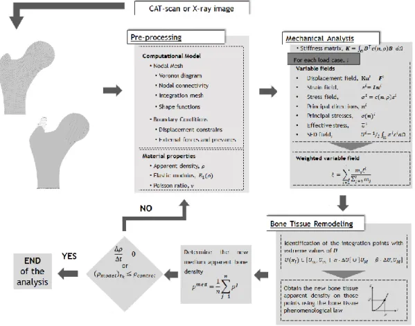
quadrilateral into an isoparametric square shape and application of the 2 x 2 quadrature point rule [12]. ... 14 Figure 5.1 – Proposed bone remodeling algorithm for the mechanical model ... 32 Figure 5.2 - (a) Voronoï cell with the quadrature points. (b) Theoretical trabecular

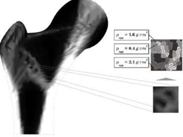
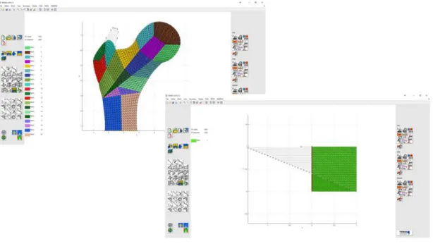
architecture of the sub-cell and homogenized apparent density. (c) Voronoï cell with the integration points homogenized apparent densities [90]. ... 33 Figure 5.3 - Isomap representing the trabecular architecture of the femoral bone. ... 34 Figure 5.4 – Some screenshots of the FEMAS graphical user interface. ... 35 Figure 5.5 – (a) Regular nodal distribution (2 481 nodes). (b) Plate model geometry and

xvi

Figure 5.6 - Evolution of the trabecular architecture with different types of mesh obtained using the FEM and the RPIM. The bone law used was Lotz’s Law with 𝜷 =

𝟎. 𝟏. ... 37

Figure 5.7 - Evolution of the trabecular architecture with increasing mesh sizes obtained using the FEM and the RPIM. The bone law used was Lotz’s Law with 𝜷 = 𝟎. 𝟏. ... 37

Figure 5.8 – Evolution of the trabecular morphology using Lotz’s law ... 38

Figure 5.9 - – Evolution of the trabecular morphology using Belinha’s law ... 39

Figure 5.10 – (a) Femoral X-ray plate. (b) Internal principal trabecular structures found in the femur bone. (c) Loads and constrains of the first mechanical case of the femur bone [12]. ... 40

Figure 5.11 – (a) Nodal distribution (1 303 nodes). (b) Model geometry and essential and natural boundary conditions. (c) Example obtained by Belinha [12] with the NNRPIM, using a nodal mesh of 5 991 nodes ... 41

Figure 5.12 – FEM solution for the first mechanical case: (a) Initial von Mises effective stress isomap; (b) Final von Mises effective stress isomap; (c) Final obtained trabecular architecture; (d) Final maximum strain isomap; (e) Final minimum strain isomap. ... 42

Figure 5.13 - RPIM solution for the first mechanical case: (a) Initial von Mises effective stress isomap; (b) Final von Mises effective stress isomap; (c) Final obtained trabecular architecture; (d) Final maximum strain isomap; (e) Final minimum strain isomap. ... 42

Figure 5.14 - NNRPIM solution for the first mechanical case: (a) Initial von Mises effective stress isomap; (b) Final von Mises effective stress isomap; (c) Final obtained trabecular architecture; (d) Final maximum strain isomap; (e) Final minimum strain isomap. ... 43

Figure 6.1 – Schematic representation of interactions between osteoclasts and osteoblasts included in Komariva’s model [96]. ... 46

Figure 6.2 - Proposed bone remodeling algorithm for the biological model. ... 51

Figure 6.3 - (a) Mesh (383 nodes) used for the analysis, in which points inside the darker area are considered bone. (b) Initial distribution of osteoclasts indicated in black. (c) Initial distribution of osteoblasts indicated in black. ... 52

Figure 6.4 - Simulation of a bone remodeling cycle: (a) Changes with time in the cell density of osteoclasts and (b) osteoblasts. The dashed line represents the steady-state solution. ... 53

Figure 6.5 - Simulation of a bone remodeling cycle: Changes with time in bone mass. ... 53

Figure 6.6 – Simulation of a bone remodeling cycle: spatial variation of bone mass along time (days). ... 54

Figure 7.1 – (a) Experimental law [101]. (b) Second order polynomial approximation. ... 56

Figure 7.2 - Proposed bone remodeling algorithm for the mechanobiological model. ... 58

Figure 7.3 - Plate model geometry and essential and natural boundary conditions ... 59

xvii

List of Tables

Table 2.1 - Autocrine and paracrine regulation during bone remodeling. ... 6

Table 2.2 - Some hormones and other local factors and their effect during bone remodeling. ... 8

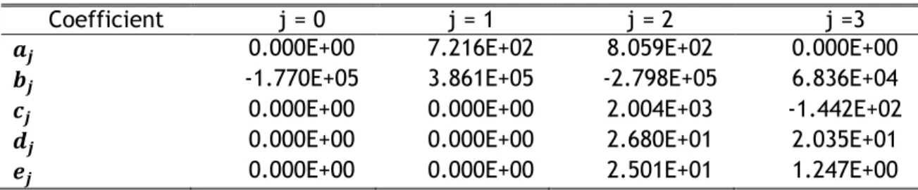
Table 5.1 - Coefficients of Lotz’s Law. ... 28

Table 5.2 - Coefficients of Belinha’s law. ... 28

Table 5.4 – Parameters of the RPIM. ... 36

Table 5.5 - Parameters of the NNRPIM. ... 36

Table 6.1 – Description of the regulatory factors considered in Komarova’s model and their respective effect on bone cell dynamics. Identification of the parameter in which each factor is considered in the model’s equations. ... 46

xix

List of Abbreviations

BMU Bone Multi-cellular Units c-fms Colony-stimulating Factor-1 DEM Diffuse Element Method

EFGM Element Free Galerkin Method FEM Finite Element Method

FEMAS Finite Element and Meshless Method Analysis Software GUI Graphical User Interface

M-CSF Macrophage Colony Stimulating Factor NEM Natural Element Method

NNFEM Natural Neighbor Finite Element Method

NNRPIM Natural Neighbor Radial Point Interpolation Method OPG Osteoprotegerin

PGE Prostaglandin E

PIM Point Interpolation Method PTH Parathyroid Hormone RANK Receptor Activator of NF-Kb RANKL Receptor Activator of NF-kB Ligand RBF Radial Basis Function

RPI Radial Point Interpolators

RPIM Radial Point Interpolation Method SED Strain Energy Density

SPH Smooth Particle Hydrodynamics TGF-β Transforming Growth Factor-β

Chapter 1

Introduction

Biomedical research, including bone biology, is most commonly “hypothesis driven”, starting always with an assumption of how a biological system might behave [4]. Knowing a

priori that the subject in study is complex, the real phenomenon has to be simplified giving

rise to a conceptual model.

In bone biology, the most famous conceptual model was proposed by Frost, known as the mechanostat theory [5]. This theory, originated from Wolff's law, states that “in a healthy subject, bone will adapt to the loads it experiences”. In his study, Frost suggested that mechanical load can be sensed by bone tissue and proposed the existence of certain feedback controls that translate information of the mechanical environment to bone cells, causing changes in bone mass and strength.

However, bone plays both local and systemic functions that interconnect with each other. Because of this, the understanding of all the different mechanisms of regulation during the bone remodeling process turns out to be extremely challenging. Also, to understand biomechanical and hormonal regulation of bone composition and architecture, studies at different dimensional scales are required [4].

So, these studies can be performed using experimental or mathematical models. This chapter compares these two types of models, weighting its advantages and limitations. Through this discussion, the motivation of this work is presented. Then, the objectives of this dissertation are presented, as well as the organization of this document.

1.1 - Motivation

After the formulation of the hypothesis, the conceptual model is tested. In life science, the rooted path is validation through experimental studies. But, in vitro and in vivo models have their strength and potential weaknesses, since they frequently use supra-physiological extremes such as maximal inhibition of specific pathways [4]. Also, interpretation of experimental data depends heavily on assumptions. For instance, it has to be assumed that the modeled processes with in vivo tests are similar to those occurring in humans, since humans cannot be directly used as experimental objects

Conscious of the limitations of experimental studies, mathematical models appear to be a promising link between conceptual models and experimental testing. In fact, mathematical

2 Introduction

modelling has proven to be a powerful tool to formalize the conceptual model and simulate proposed experiments in silico. Thus, mathematical modelling allows the validation of a conceptual model, the identification of the most influential parameters and ultimately the prediction of an experimental outcome consistent with the conceptual model. Additionally, these models have shown to be a valuable help when different events with different time scales are being simultaneously studied and when the system exhibits non-linear behavior, like the case of bone remodeling. Also, when exists a solid connection between mathematical and experimental models, the consequent flow of information between them lead to biological systems with highly enhanced accuracy. However, as the complexity of the question under investigation increases, the required mathematical model has to be more sophisticated and complex.

But, when weighting the advantages and the limitations of these models, the numerous possibilities that they can offer prevail. And, in fact, it was those promising and, in many cases, already proven results, that fed the motivation for this work.

1.2 - Objectives

The main objective of this project is to develop a new mechanobiological model to predict the bone tissue remodeling process, reproducing accurately the biological response in the presence of a mechanical stimulus.

Therefore, to accomplish this goal, several secondary objectives were stipulated, such as:  Understand the influence of stress in bone tissue during a remodeling

phenomenon;

 Develop a bone tissue remodeling algorithm only taking in consideration mechanical stimuli;

 Validate the mechanical model through a 2D analysis, using different numerical methods;

 Study the relevance of hormonal/chemical external effects;

 Develop a 2D diffusion model of bone remodeling considering the cellular behavior of bone cells;

 Validate the biological model through a 2D analysis, using different numerical methods.

1.3 - Document Structure

The thesis was organized in several chapters, starting with Chapter 1, in which the theme in study and the main objectives of the work are presented. Chapter 2 describes the biological process of bone remodeling and its mechanisms of regulation. Chapter 3 focus on the three numerical methods used in this work, describing briefly their formulation, followed by, in Chapter 4, an introduction of basic notions of solid mechanics. Then, in Chapters 5 and 6, respectively, the mechanical and the biological models created are presented, as well as the results obtained for each model. In Chapter 7, the focus is on a full description of the new mechanobiological model proposed in this work. To finish, in Chapter 8, the main achievements of the work are presented along with the suggestion of future work that could be implemented.

Chapter 2

Bone Tissue

Bone is a highly reactive tissue. The relationship between bone mechanical environment and bone internal and external structure was first described by J.Wolff, who suggested that bone grows wherever needed and decreases where is not needed [6].

Thus, the subject of this chapter is bone and its remodeling process. Additionally, both biological and mechanical regulation will be described.

2.1 - Bone Morphology

The skeletal system is constituted by bone and cartilage and has two main functions in the organism - mechanical and metabolic. Regarding the first one, skeletal system allows support and protection of vital internal organs, as well as muscle attachment for locomotion [7]. The skeleton is also considered a mineral repository, especially of calcium and phosphate, having an important metabolic action for the maintenance of serum homeostasis. Additionally, in the red marrow of the bone, blood cells, such as erythrocytes, leucocytes and platelets, are produced [8].

Bone is a porous mineralized structure made up of cells, vessels, collagen and crystals of calcium compounds (hydroxyapatite) [7]. The variation of their proportion originates two different types of bone – cortical and trabecular. Thus, although having identical chemical composition, this variation causes different structural macroscopically and microscopically organizations.

Cortical bone comprises 80% of the skeleton and can be found in the outer part of all skeletal structures. The basic functional unit of cortical bone is the osteon, which consists of concentric layers of bony lamellae surrounding a central Haversian canal, which contains the blood capillaries that supply the bone tissue. It has a slow turnover rate and is a compact material, as represented in Figure 2.1a. Its high density leads to a high resistance to bending and torsion. On the other hand, trabecular bone represents 20% of the skeletal mass and is a complex network of intersecting curved plates and tubes in the inner part of the skeletal structures (Figure 2.1b). When compared to cortical bone, it is less dense and more elastic. Also, while cortical bone has an important mechanical function, trabecular bone exhibits a major metabolic function, having a higher turnover rate. Lastly, regardless of its relatively small volume and high apparent porosity, trabecular bone is well adapted to resist and

4 Bone Tissue

conduct compressive loads. In long bones, trabecular bone is typically located at the proximal ends, having an arrangement relatively regular that reflects the direction of the principal mechanical stresses to which this kind of bone is being subjected [8].

Lastly, bone is a living tissue experimenting a continuous reconstruction and reformulation along its life span [9]. Therefore, to maintain the shape, quality and size of the skeleton bone is constantly remodeling.

2.2 - Bone Remodeling

Bone remodeling is a complex process by which old bone is continuously replaced by new tissue, repairing micro fractures and modifying its structure in response to stress and other biomechanical forces. The process is sequential, as can be depicted in Figure 2.2, starting by an activation phase followed by resorption, reversal and formation phases. The bone cells active in the process are the osteoclasts and the osteoblasts, which are temporally and spatially coupled, closely collaborating within bone multi-cellular units (BMUs). The organization of the BMUs in cortical and trabecular bone is morphologically different, since trabecular bone is more actively remodeled than cortical bone. Nevertheless, there are no differences between the two types of bone when it comes to the biological events during bone remodeling [7].

The remodeling cycle begins with the resorption phase, in which osteoclasts have the leading role. Osteoclasts are giant multinucleated cells, derived from hematopoietic cells of the mononuclear lineage [10] and are the bone lining cells responsible for bone resorption. Thus, the resorption phase starts with the activation of a quiescent bone surface through a cascade of signals to osteoclastic precursors, causing their migration to the bone surface, where they form multinucleated osteoclasts [11] (Figure 2.2a). Simultaneously, bone-lining cells disappear from the bone surface, allowing osteoclasts to adhere to the bone matrix and resorb bone [7] (Figure 2.2b).

After the completion of the resorption, mononuclear cells appear on the bone surface releasing signals for osteoblast differentiation and migration (Figure 2.2c). This phase is

a )

b )

Figure 2.1 - Transversal cross-section of an osteon (a) and a trabecular branch (b)

Bone Remodeling 5 known as the reversal phase, since it prepares the bone surface for the arrival of new osteoblasts and consequently the formation of new bone [7].

Osteoblasts are the cells responsible for the production of bone matrix constituents and are originated from multipotent mesenchymal stem cells. During the formation phase, osteoblasts lay down bone until the resorbed bone is completely replaced by new one (Figure 2.2d). In this phase, osteoblasts start by synthesizing and depositing collagen. Then, the production of collagen decreases, and a secondary full mineralization of the matrix takes place. In this step, the collagen matrix built previously acts as the scaffold in which minerals such as phosphate and calcium begin to crystalize to form bone [7], [11]. Toward the end of the matrix-secreting period (Figure 2.2e), 15% of mature osteoblasts are entrapped in the new bone matrix and differentiate into osteocytes, while some cells remain on the bone surface, becoming flat lining cells [7].

a) b)

c) d) e)

Figure 2.2 – Bone remodeling process [12]

2.2.1 -

Regulation Mechanisms

So, during a remodeling cycle, the turnover of bone is managed by a sequential process performed by the bone cells within a BMU, in which the activities of bone-forming osteoblasts and bone-resorbing osteoclasts have to be coordinated. These activities of osteoblasts and osteoclasts are controlled by a variety of hormones and cytokines, as well as by mechanical loading [13].

For instance, during the resorption phase, protein and mineral components of bone and various local paracrine and autocrine regulatory factors are released, such as the receptor activator of NF-kB ligand (RANKL), the receptor activator of NF-Kb (RANK) or the osteoprotegerin (OPG) [11].

The RANKL/RANK interaction is, in fact, critical for this resorption phase. Protein RANKL is a ligand for RANK on hematopoietic cells, and it is the primary driver of formation, activation and survival of osteoclasts [14]–[19]. So, the major biological action of RANKL,

6 Bone Tissue

together with the protein ligand macrophage colony stimulating factor (M-CSF) is to induce osteoclast activation and in this way promote bone resorption [16], [20], [21]. RANK receptor is found on the surface of osteoclastic progenitors and osteoclasts, while the major source of RANKL in physiologic bone remodelling are cells of the stromal/osteoblastic lineage. However, other cells may act as a source of RANKL in pathologic states.

To counteract the differentiation and activation of osteoclasts, osteoblasts produce and secrete OPG, a decoy receptor that can block RANKL/RANK interactions [11], [14]. The critical biological role of OPG is then the inhibition of osteoclast function and the acceleration of osteoclast apoptosis [22]. Therefore, the OPG/ RANKL/ RANK system is considered the major regulatory system in which the coordination of osteoclastogenesis and bone remodelling converges [23]–[25], as can be depicted in Figure 2.3

Despite this, there are limitations regarding this system since it is difficult, if not impossible, to assess the RANKL and OPG status in patients without invasive procedures such as bone biopsies. In Table 2.1, the OPG/RANKL/RANK is resumed, defining the principal action of each regulatory factor and its origin.

Table 2.1 - Autocrine and paracrine regulation during bone remodeling.

Factor Origin Action

RANKL Surface of stromal/osteoblastic

lineage Activation of osteoclasts

RANK Surface of osteoclastic lineage

OPG Secreted by osteoblasts Inhibition of osteoclasts

Besides these local paracrine and autocrine effectors, local cytokines and growth factors have also an important role in bone remodelling, acting either as stimulators or as inhibitors of bone resorption or bone formation. Some of these factors act independently of the cytokines RANKL and OPG, and are necessary factors in the recruitment and differentiation of osteoblastic and osteoclastic cells. A subset of examples include members of the transforming

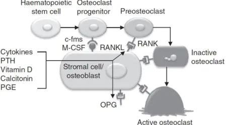
Figure 2.3 - Regulation of osteoclast formation and activity as a result of the OPG/RANKL/RANK

system. Cells of the osteoblastic lineage initiate bone remodeling by contact with osteoclastic progenitors. M-CSF stimulates the colony-stimulating factor-1 (c-fms) receptor on osteoclasts. Osteoclast differentiation and activity are stimulated by RANK/RANKL interaction, and this interaction can be blocked by soluble OPG. Osteoclastogenesis is influenced by various systemic hormones and local factors such as cytokines, parathyroid hormone (PTH), vitamin D, calcitonin and prostaglandin E (PGE) [9], [15].

Bone Remodeling 7 growth factor-β (TGF-β) family, tumour necrosis factor-α, various interleukins, insulin-like growth factors I and II, prostaglandin E2 and M-CSF [14], [23]–[31]. For instance, TGF- β belongs to a family of closely related polypeptides, in which TGF- β 1, 2, and 3 have similar effects on bone cell function [32]. TGF-β is released by osteoclasts during bone resorption [33] making bone matrix the largest source of TGF-β in the body [34]. Its effect on osteoblasts is bi-directional depending upon the state of maturation of osteoblasts [35]. In vivo studies have confirmed a stimulatory effect of TGF-β on bone formation [36]–[38], suggesting a potential to stimulate osteoblast recruitment, migration and proliferation of osteoblast precursors [33], [39]. On the other hand, it was also found that TGF-β inhibits terminal osteoblastic differentiation [40], by inhibiting alkaline phosphatase activity and osteocalcin synthesis [32]. The actions of TGF-β on bone resorption has a biphasic effect on osteoclastogenesis [32]. At low concentrations it enhances osteoclast formation, whereas at high concentrations induces osteoclast apoptosis [34], [41].

Along with this local regulation, bone remodelling involves also a systemic regulation controlled by hormones, such as estrogen and calcium-regulating hormones. It is known that activation of estrogen receptors in osteoclast progenitor cells decreases osteoclast formation and enhances apoptosis. Also, activation of estrogen receptors in terminally differentiated osteoclasts inhibits their bone-resorbing activity [13], [42]–[45]. But, although the loss in bone mass caused by estrogen deficiency is primarily due to enhanced bone resorption, decreased bone formation is also a contributing factor [46], [47]. It has been shown that stimulation of estrogen receptors in osteoblasts activates their anabolic activities and decreases the pathway by which osteoblasts can activate osteoclasts [13]. Estrogen also stimulates the expression of type I collagen, and decreased levels of estrogen would result in osteoblasts less active in producing an extracellular matrix [48]. Activation of the estrogen receptors in osteoblasts/stromal cells may also play a role in the regulation of osteoclastogenesis, by decreasing the expression of M-CSF [49]–[51]. This way, accordingly to this data, it is possible to conclude that estrogen is crucial for keeping bone mass in balance.

But, there are other systemic hormones that affect bone turnover. The mineral homeostatic mechanisms in the skeleton are controlled by the calcium-regulating hormones, which are PTH, calcitriol, that is the active hormonal form of 25-OH-vitamin D, and calcitonin, the active metabolite of 25-OH-vitamin D [24].

PTH is an important regulator of calcium homeostasis and rapidly influences its concentrations since stimulates bone resorption by increasing renal calcium reabsorption [11]. However, the study of the actions of PTH when administered in the organism is more complex due to its multiple effects. When given continuously, PTH induces bone loss, whereas in intermittent applications it stimulates bone gain. On the other hand, calcitriol exerts a tonic inhibitory effect on PTH synthesis and is necessary for optimal intestinal absorption of calcium and phosphorus [52]. Ultimately, calcitonin increases the transformation of 25-OH-vitamin D to its active metabolite, leading indirectly to an increase in calcium concentrations [7], [25], [26], [53], [54].

In Table 2.2, it is resumed the main actions of some of the hormones and cytokines talked above and their influence on the activities of osteoblasts and osteoclasts

8 Bone Tissue

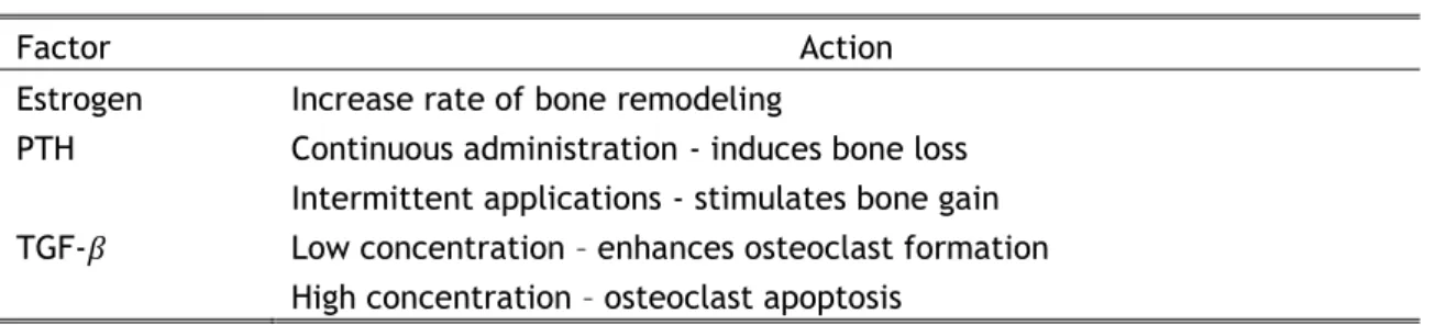
Table 2.2 - Some hormones and other local factors and their effect during bone remodeling.

Factor Action

Estrogen Increase rate of bone remodeling

PTH Continuous administration - induces bone loss Intermittent applications - stimulates bone gain TGF-𝛽 Low concentration – enhances osteoclast formation

High concentration – osteoclast apoptosis

Lastly, mechanical loading is also a very important factor to take into account, since osteocytes respond to bone tissue strain and enhance bone remodelling activity [7]. Therefore, osteocytes convert mechanical stimuli into metabolic responses, organizing bone turnover under mechanical strain and immobilization [53], [55], [56]. Being descended from osteoblasts, they have similar paracrine capabilities, influencing the balance between RANKL and OPG regarding bone turnover mechanism. Increased mechanical strain inhibits RANKL and upregulates OPG, which decreases osteoclastic activity and therefore increases bone mass indirectly through the osteocytes [7]. Loading plays then an important role. A low amount of loading leads to bone loss, due to decreased anabolic activity of osteoblasts and increased osteoclastic resorption, and high loading causes increased bone mineral density, due to the anabolic activation of osteoblasts [13].

In conclusion, remodeling is a lifelong coordinated and dominant process in the adult skeleton, initiated by resorption and followed by new bone formation at the same site where the resorption process occurred [24]. Bone remodeling is important for the maintenance of bone mass, to repair micro damage of the skeleton, to prevent accumulation of too much old bone and for mineral homeostasis [24].

Chapter 3

Numerical Methods

Many phenomena in nature such as heat conduction, stress in mechanical structures, electromagnetic fields or fluid mechanics involve either domains of two or more dimensions or nonlinear effects [57]. Thus, to simulate these processes it is required to use partial differential equations or nonlinear differential equations, and the bone remodelling process is no exception. But, in general, none of these equations can be solved symbolically or analytically, so researchers need to use numerical methods [57]. Thanks to the advancement of high-speed digital computers, the cost-effectiveness of numerical procedures has been greatly enhanced, and these methods have become very accurate and reliable [58].

In the work developed, the numerical methods used were determinant to the success of the simulation models created. So, this chapter begins with a very brief introduction about the FEM, followed by a more detailed analysis of two meshless methods, namely the RPIM and the (NNRPIM), reporting some of the most important concepts of these two numerical methods.

3.1 - FEM

As previously mentioned, with the increase in complexity of the problems studied, the need of a method of approximation to solve these continuum problems was urgent. This led to the first definition of a unified treatment of "standard discrete problems", known as FEM.

FEM approach breaks the domain into a finite number of pieces called elements, and uses basis functions, usually piecewise polynomials that are local to each element [59], [60]. FEM is then characterized by the discretization of the domain into several subdomains called finite elements [58], that construct a mesh, as illustrated in Figure 3.1. These elements can be irregular and possess different properties enabling the discretization of structures with mixed properties [58].

10 Numerical Methods

FEM has been used with great success on many fields of engineering. However, this method is not free of limitations. The main one is related with the mesh based-interpolation [61]. Special attention has to be given to the quality of the mesh, because low quality meshes lead to high values of error. Being a classical mesh-based method, FEM is not suitable to treat problems with discontinuities that don't align with element edges [61].

3.2 - Meshless Methods

Since FEM’s performance relies greatly on the quality of the mesh, other numerical methods were created and offered as solid options. Meshless methods were one of the options created, in which the problem physical domain is discretized in an unstructured nodal distribution and the field functions are approximated within an influence-domain rather than an element [12], [62], [63].

Regarding the formulation, meshless methods can be classified in two categories. The first one is the strong formulation in which the partial differential equations describing the phenomenon are used directly to obtain the solution [12]. One of the first meshless methods created in this category was the smooth particle hydrodynamics (SPH) method. A parallel path on the development of meshless methods was initiated in the 1990's using this time a weak form solution. In weak formulation, each differential equation has a residual weight to be minimized. The residual is not given by the exact solution of the differential but by an approximated function affected by a test function [12]. The first meshless method using this formulation was the Diffuse Element Method (DEM) proposed by Nayroles [64]. Belytschko extended this method and proposed one of the most well-known methods, the Element Free Galerkin Method (EFGM) [65].

Meshless methods described above are approximants, and in spite of the successful applications of these type of meshless methods in computational mechanics, some problems remained unsolved, being the lack of the Kronecker delta property on the approximation functions the most important one [12].

Due to this fact, several interpolant meshless methods were developed, such as Point Interpolation Method (PIM) [66], the RPIM [67], [68], Natural Neighbour Finite Element Method (NNFEM) [69], [70] and the Natural Element Method (NEM) [71], [72]. The combination between the NEM and the RPIM originated the NNRPIM [12], [73].

Meshless Methods 11

3.2.1 -

Meshless Generic Procedure

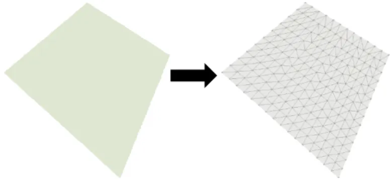
To initialize the process, the only information required is the spatial location of each node discretizing the problem domain. It is important to notice that this nodal distribution do not form a mesh, since it is not required any kind of previous information about the relation between each node in order to construct the approximation or interpolation functions of the unknown variable field functions [12]. In Figure 3.2, it is possible to observe an illustration of this process.

a) b) c)

Figure 3.2 - (a) Solid domain. (b) Regular nodal discretization. (c) Irregular nodal discretization [12].

After the discretization, nodal connectivity can be imposed using either influence-domains or Voronoї diagrams. Then, the construction of a background integration mesh is needed. As in FEM, it is common to use Gaussian integration meshes fitted to the problem domain. But there are other techniques, such as the use of the nodal integration, resorting to the Voronoï diagrams in order to obtain the integration weight on each node [12]. The following step is the establishment of the equation system, that can be can be formulated using approximation or interpolation functions. The interpolation functions possess an important property, namely Kronecker delta property, meaning that the function obtained passes through all scattered points in an influence domain. This property is an important advantage, since it allows the use of the same simple techniques used in FEM to impose the essential boundary conditions.

Thus, after a brief analysis of the generic procedure of meshless methods, it is possible to conclude that a meshless method requires the presence and combination of three basic parts: nodal connectivity, numerical integration scheme and shape functions. These three concepts will be analyzed and, since RPIM and NNRPIM differ in respect to both nodal connectivity and numerical integration scheme, the following sections will explain with detail these differences.

3.2.2 -

Nodal Connectivity

3.2.2.1 - RPIM

The RPIM is based on the Galerkin weak form formulation using meshfree shape functions constructed using radial basis functions (RBF).

12 Numerical Methods

In RPIM, the nodal connectivity is obtained by the overlap of the influence-domain of each node. Influence-domains are found by searching enough nodes inside a certain area or volume, and can have a fixed or a variable size. Many meshless methods [67], [74], [75] use fixed size influence-domains, but RPIM uses a fixed number of neighbor nodes instead.

Regarding fixed size influence-domains, in Figure 3.3, it is presented an example of two types of fixed size domains, a rectangular (Figure 3.3a) and a circular (Figure 3.3). By analyzing these figures, it is possible to note that influence-domains with different shapes and sizes originate different nodal connectivities. Also, depending on the initial nodal spatial distribution, influence-domains obtained can be unbalanced, not containing an approximately constant number of nodes. All of these factors can affect the final solution of the problem and cause loss of accuracy in the numerical analysis.

Therefore, to overcome these limitations, RPIM uses variable size influence-domains, with constant number of nodes inside the domain. Thus, performing a radial search and using the interest point 𝒙𝐼 as center, the n closest nodes are found. In Figure 3.3c, this process is illustrated, culminating in a constant nodal connectivity that avoids the numerical problems identified previously.

a) b) c)

Figure 3.3 - Examples of different types of domains: (a) fixed rectangular shaped

influence-domain, (b) fixed circular shaped influence-domain and (c) flexible circular shaped influence-domain [12].

3.2.2.2 - NNRPIM

The NNRPIM is an advanced discretization meshless technique combining the natural neighbor geometric concept with the radial point interpolators (RPI) [76].

Nodal connectivity is obtained using the natural neighbor concept with the partition of the discretized domain into a set of Voronoї cells [77]. To each one of these cells is associated one and only one node [76]. Considering a problem domain Ω ⊂ ℝ2_{, bounded by a} physical boundary Γ ∈ Ω, discretized in several randomly distributed nodes 𝑁 = {𝑛0, 𝑛1, … , 𝑛𝑁} ∈ ℝ2 with the following coordinates: 𝑋 = {𝑥0, 𝑥1, … , 𝑥𝑁} with 𝑥𝑖∈ ℝ2, the Voronoї cell is defined by

Meshless Methods 13 being 𝒙𝐼 an interest point of the domain and ∥ ⋅ ∥ the Euclidian metric norm [12]. Thus, the Voronoï cell 𝑉𝑖 is the geometric place where all points in the interior 𝑉𝑖 are closer to the node 𝑛𝑖 than to any other node [12]. The assemblage of the Voronoї cells define the Voronoї diagram. Thus, the Voronoï diagram of N is the partition of the domain defined by Ω into sub regions 𝑉𝑖 , closed and convex, as can be seen in Figure 3.4a.

a) b) c)

Figure 3.4 - (a) Second degree influence cell of interest point 𝐱𝐈. (b) Representation of the sub-cells

forming the Voronoï cell. (c) Schematic representation of 4 × 4 integration points inside a sub-cell [76].

In the NNRPIM, influence cells are organic influence-domains that are built using the information from the Voronoї diagram, making them dependent on the nodal mesh arrangement.

In this work, it was determined the "second degree influence-cell". To establish them, a point of interest, 𝒙𝐼, starts by searching for its neighbour nodes following the Natural Neighbor Voronoï construction, considering only its first natural neighbors. Then, based again on the Voronoï diagram, the natural neighbors of the first natural neighbors of 𝒙𝐼 are added to the influence-cell, as it is represented in grey in Figure 3.4a.

3.2.3 -

Numerical Integration

3.2.3.1 - RPIM

For the numerical integration, RPIM uses the Gauss-Legendre quadrature scheme. Initially, the solid domain is divided in a regular grid as Figure 3.5a indicates. Then, each grid-cell is filled with integration points, respecting the Gauss-Legendre quadrature rule, as illustrated in Figure 3.5b.

14 Numerical Methods

a) b)

Figure 3.5 - (a) Gaussian integration mesh and (b) transformation of the initial quadrilateral into an

isoparametric square shape and application of the 2 x 2 quadrature point rule [12].

The Cartesian coordinates of the quadrature points are obtained using isoparametric interpolation functions, 𝑁𝑖, present in Equations (3.2) and (3.3).

𝑁1(𝜉, 𝜂) = 1 4(1 − 𝜉)(1 − 𝜂) 𝑁2(𝜉, 𝜂) = 1 4(1 − 𝜉)(1 + 𝜂) _(3.2) 𝑁3(𝜉, 𝜂) = 1 4(1 + 𝜉)(1 + 𝜂) 𝑁4(𝜉, 𝜂) = 1 4(1 + 𝜉)(1 − 𝜂) 𝑁1(𝜉, 𝜂) = 1 − 𝜉 − 𝜂) 𝑁2(𝜉, 𝜂) = 𝜂 _(3.3) 𝑁3(𝜉, 𝜂) = 𝜉 The Cartesian coordinates are given by

𝑥 = ∑ 𝑁𝑖(𝜉, 𝜂) ∙ 𝑥𝑖 𝑚 𝑖=1 (3.4) 𝑦 = ∑ 𝑁𝑖(𝜉, 𝜂) ∙ 𝑦𝑖 𝑚 𝑖=1

in which m is the number of nodes inside the grid-cell and 𝑥𝑖 and 𝑦𝑖 are the Cartesian coordinates of the cells nodes.

The integration weight of the quadrature point is obtained by multiplying the isoparametric weight of the quadrature point with the inverse of the Jacobian matrix determinant of the respective grid-cell, as described in the Equation (3.5).

Meshless Methods 15 [𝐽] = ( 𝜕𝑥 𝜕𝜉 𝜕𝑥 𝜕𝜂 𝜕𝑦 𝜕𝜉 𝜕𝑦 𝜕𝜂) (3.5) 3.2.3.2 - NNRPIM

Since the NNRPIM uses the Galerkin weak form, a background integration mesh is necessary. In this method, the integration mesh is obtained using directly and exclusively the nodal distribution, namely the previously constructed Voronoï diagram [78]. Using the Delaunay triangulation, the area of each Voronoï cell is subdivided in several sub-areas. Thus, each area of the Voronoï cell of node 𝒙𝑗, 𝐴𝑉𝑗, is divided into k sub-areas A_i

V_j

, in which 𝐴𝑉𝑗 ₌

∑𝑘 AV_ij

𝑖=1 , as can be seen in Figure 3.4b. Then, following the Gauss–Legendre quadrature rule, it is possible to distribute integration points inside each subarea AV_ij_{. In Figure 3.4c, it is}

exemplified a 4x4 distribution. By repeating the mentioned procedure for the N Voronoï cells from the Voronoï diagram, the background integration mesh discretizing the problem domain is obtained.

In this work, the integration mesh is constructed considering just one integration point per sub-area AV_ij_{, since previous research works on the NNRPIM show that this simple}

integration scheme is sufficient to integrate accurately the integro-differential equations [73], [76].

3.2.4 -

Interpolation Functions

Considering the RPIM and the NNRPIM, the interpolation functions for both methods possess the Kronecker delta property, satisfying the following condition,

𝜑𝑖(𝒙𝑗) = 𝛿𝑖𝑗 (3.6)

where 𝛿𝑖𝑗 is the Kronecker delta, 𝛿𝑖𝑗 = 1 if 𝑖 = 𝑗 and 𝛿𝑖𝑗 = 0 if 𝑖 ≠ 𝑗. This property simplifies greatly the process of imposition of the essential boundary conditions, because it allows to apply them directly in the stiffness matrix.

The interpolation functions for both methods are determined using the RPI technique [67], which requires the combination of a polynomial basis with a RBF. So, considering the function 𝑢 (𝒙𝐼) defined in the domain 𝛺 ⊂ ℝ2, the value of function 𝑢 (𝒙𝐼) at the point of interest 𝒙𝐼 is defined by 𝑢(𝒙𝐼) = ∑ 𝑅𝑖(𝒙𝐼) ∙ 𝑎𝑖(𝒙𝐼) + ∑ 𝑝𝑗(𝒙𝐼) 𝑚 𝑗=1 ∙ 𝑏𝑗(𝒙𝐼) = 𝑹𝑇(𝒙𝐼) ∙ 𝒂(𝒙𝐼) + 𝒑𝑇∙ 𝒃(𝒙𝐼) 𝑛 𝑖=1 (3.7)

where 𝑅𝑖(𝒙𝐼) is the RBF, 𝑝𝑗(𝒙𝐼) is the polynomial basis function and 𝑎𝑖(𝑥𝐼) and 𝑏𝑗(𝒙𝐼) are non-constant coefficients of 𝑅𝑖(𝑥𝐼) and 𝑝𝑗(𝒙𝐼), respectively [76]. The variable defined on the RBF is the distance 𝐫𝐈𝐢 between the relevant node 𝒙𝑰 and the neighbour node 𝑥𝑖, given by rIi= |𝒙𝑖− 𝒙𝐼|. The RBF used in this work is the Multiquadric RBF [79], 𝑅𝑖(𝑥𝐼) = 𝑅(rIi) = (𝑟𝐼𝑖2+ 𝑐2)𝑝, in which shape parameter c takes a value close to zero, 𝑐 ≅ 0, and p close to one, 𝑝 ≅ 1 [73], [80]. Regarding the Equation (3.7), it is still needed to obtain the non-constant coefficients 𝒂 and 𝒃. The polynomial basis functions used have the following monomial term as

16 Numerical Methods

𝒑𝑇_(𝒙

𝐼) = [1, 𝑥, 𝑦, 𝑥2, 𝑥𝑦 , 𝑦2, … ] (3.8) Considering Equation (3.7) for each node inside the influence-cell domain and including an extra equation, ∑𝑛𝑖=1𝑝𝑗(𝒙𝐼)𝑎𝑖= 0, in order to guarantee a unique solution [81], a system of equations defined in Equation (3.9) is obtained.

[𝑹 𝒑 𝒑𝑇 ₀] { 𝒂 𝒃} = { 𝒖𝑺 0} (3.9)

Through this system of equations, and being the vector of the nodal function values for the nodes on the influence-cell defined by: 𝒖𝑆= {𝑢1, 𝑢2 … 𝑢𝑛}𝑇 these coefficients are determined (Equation (3.10). {𝒂_𝒃} = [𝑹 𝒑 𝒑𝑇 ₀] −1 {𝒖₀𝑺} ⟹ {𝒂_𝒃} = 𝑴−1_{𝒖𝑺 0} (3.10)

Recalling that a certain field variable value for an interest point 𝒙𝐼 is interpolated using the shape function values obtained at the nodes inside the support domain of 𝒙𝐼, it is now possible to define the interpolation function, by substituting in Equation (3.7) the result from Equation (3.10). The interpolation function 𝚽(𝒙𝐼) = {𝜑1(𝒙𝐼), 𝜑2(𝒙𝐼), … , 𝜑𝑛(𝒙𝐼)} for an interest point 𝒙𝐼 is then defined by

𝑢(𝒙𝐼) = {𝑹𝑇(𝒙𝐼), 𝒑𝑇(𝒙𝐼)} 𝑴−1{ 𝒖𝑆

0} = 𝚽(𝒙𝐼) { 𝒖𝑆

0} (3.11)

In order to compute the partial derivatives of the interpolated field function, it is necessary to obtain the respective RPI shape functions partial derivatives. So, using for the problem 2D that is being studied, the partial derivative of 𝚽(𝒙𝐼) is defined as

𝚽,𝒙(𝒙𝐼) = {𝑹𝑇(𝒙𝐼) 𝒑𝑇(𝒙𝐼)},𝑥 𝑴−1 (3.12)

𝚽,𝒚(𝒙𝐼) = {𝑹𝑇(𝒙𝐼) 𝒑𝑇(𝒙𝐼)},𝑦 𝑴−1 (3.13) The first order partial derivative of the RBF vector with respect to the same 2D problem is defined as 𝑹(𝒙𝐼),𝑥= {𝑹1(𝒙𝐼),𝑥 𝑹2(𝒙𝐼),𝑥 ⋯ 𝑹𝑛(𝒙𝐼),𝑥} 𝑇 = {𝜕𝑹1(𝒙𝐼) 𝜕𝑥 𝜕𝑹2(𝒙𝐼) 𝜕𝑥 ⋯ 𝜕𝑹𝑛(𝒙𝐼) 𝜕𝑥 } 𝑇 (3.14) 𝑹(𝒙𝐼),𝒚= {𝑹1(𝒙𝐼),𝒚 𝑹2(𝒙𝐼),𝒚 ⋯ 𝑹𝑛(𝒙𝐼),𝒚} 𝑇 = {𝜕𝑹1(𝒙𝐼) 𝜕𝑦

⋯

Meshless Methods 17 𝜕𝑅𝑖(𝒙𝐼) 𝜕𝑥 = −2𝑝(𝑟𝑖𝐼 2_{+ 𝑐}2₎𝑝−1_(𝑥 𝑖− 𝑥𝐼) (3.16) 𝜕𝑅𝑖(𝒙𝐼) 𝜕𝑦 = −2𝑝(𝑟𝑖𝐼 2_{+ 𝑐}2₎𝑝−1_(𝑦 𝑖− 𝑦𝐼) (3.17)

Chapter 4

Solid Mechanics

The continuum mechanics is the foundation of the nonlinear numerical analysis. It is known that solids and structures subjected to loads or forces become stressed. These stresses lead to strains, which can be interpreted as deformations or relative displacements [12].

Since load plays an important role in bone remodeling, in this chapter, the concepts of strain and stress are introduced, followed by an explanation of the equilibrium and the constitutive equations used.

4.1 - Fundamentals

The study of Solid Mechanics is mainly devoted on the relationships between stress and strain and strain and displacements, for a given solid and boundary conditions (external forces and displacements constrains) [82], [83]. So, when analyzing a deformation, the consequent change in the body configuration is defined by the stress and the strain terms. This way, the virtual work can be expressed as an integral over the known body volume. It is important to guarantee that both strain tensor and stress tensor are referred to the same deformed state. To represent the stresses of the current configuration, the symmetric Cauchy stress tensor, 𝚲, can be defined

𝚲 = [𝜎_𝜎𝑥𝑥 𝜎𝑥𝑦

𝑦𝑥 𝜎𝑦𝑦] (4.1)

This work, uses the Voigt notation, expressing tensors in column vectors. Therefore, stress tensor 𝚲 is reduced to the stress vector 𝝈,

𝝈 = {𝜎𝑥𝑥 𝜎𝑦𝑦 𝜎𝑥𝑦 } 𝑇

(4.2)

and the strain tensor 𝑬 to the strain vector 𝜺,

𝜺 = {𝜀𝑥𝑥 𝜀𝑦𝑦 𝜀𝑥𝑦 } 𝑇

20 Solid Mechanics

Solids can show different behaviors, depending on the solid material. In this work only linear elastic isotropic materials are considered. Isotropic materials can be fully described by only two independent material properties, the Young modulus, 𝐸, and the Poisson ratio, 𝜈. Thus, the relation between stress and strain in the solid domain is given by the constitutive equation, known as Hooke's Law

𝝈 = 𝒄𝜺 (4.4)

in which, 𝒄 is the constitutive matrix, given by 𝒄 = 𝒔−1_{, being the matrix 𝒔 the compliance} elasticity matrix. For a general anisotropic material case and considering a plane stress formulation, matrix 𝒔 is given by

𝒔𝑝𝑙𝑎𝑛𝑒 𝑠𝑡𝑟𝑒𝑠𝑠 = [ 1 𝐸11 −𝜐21 𝐸22 0 −𝜐12 𝐸11 1 𝐸22 0 0 0 1 𝐺12] (4.5)

while, when considering a plane strain formulation, matrix 𝒔 is given by

𝒔𝑝𝑙𝑎𝑛𝑒 𝑠𝑡𝑟𝑎𝑖𝑛 = [ 1 − 𝜈31𝜈13 𝐸11 −𝜐12+ 𝜈31𝜈23 𝐸22 0 −𝜐12+ 𝜈32𝜈13 𝐸11 1 − 𝜈32𝜈23 𝐸22 0 0 0 1 𝐺12] (4.6)

being 𝐸𝑖𝑗 the elasticity modulus, 𝜈𝑖𝑗 the material Poisson coefficient and 𝐺𝑖𝑗 the distortion modulus in material direction 𝑖 and 𝑗.

Obtaining the constitutive matrix 𝒄, it is possible to align it with a new material referential 𝑂𝑥′𝑦′ defined by the versors 𝒊 = {𝑖′𝑥, 𝑖′𝑦} and 𝒋 = {𝑗′𝑥, 𝑗′𝑦}, using the following expression

𝒄′_{= 𝑻}𝑇_{𝒄 𝑻 (4.7)}

being 𝑻 the transformation matrix given by

𝑻 = [

cos2_{𝛼 sen}2_{𝛼 − sin 2𝛼}

sen2_{𝛼 cos}2_{𝛼 sin 2𝛼}

sin 𝛼 ∙ cos 𝛼 −sin 𝛼 ∙ cos 𝛼 cos2_{𝛼 ∙ sen}2_𝛼

] (4.8)

where the angle 𝛼 is the angle between the original material axis 𝑂𝑥 and the new material axis 𝑂𝑥’:𝛼 = cos−1_{(𝒊, 𝒊′).}

Now, considering the displacement field given by 𝒖 = {𝑢, 𝑣, 𝑤}, strain components are expressed as

𝜀𝑥𝑥= 𝜕𝑢 𝜕𝑥

Weak Form 21 𝜀𝑦𝑦= 𝜕𝑣 𝜕𝑦 𝜀𝑥𝑦= 𝜕𝑢 𝜕𝑦+ 𝜕𝑣 𝜕𝑥

Thus, the strain vector can be defined by the combination of a differential operator and the displacement field, 𝒖,

𝜺 = 𝑳𝒖 (4.10) where 𝑳 is given by 𝑳 = [ 𝜕 𝜕𝑥 0 𝜕 𝜕𝑦 0 𝜕 𝜕𝑦 𝜕 𝜕𝑥] 𝑇 (4.11)

4.2 - Weak Form

The strong form system equations are the partial differential system equations governing the studied physic phenomenon. Using this formulation, the exact solution is always obtained. However this is usually an extremely difficult task in complex practical engineering problems.

On the other hand, formulations based on weak forms give a discretized system of equations but with a weaker consistency on the adopted approximation (or interpolation) functions. This formulation is able to produce stable algebraic system equations and more accurate results [12].

4.2.1 -

Galerkin Weak Form

In this work, the discrete equation system is obtained using the Galerkin weak form, which is a variational method based on energy minimization.

So, considering a body described by the domain Ω ∈ ℝ2 _{and bounded by Γ, where} Γ ∈ Ω: Γ𝑢∪ Γ𝑡= Γ ∧ Γ𝑢∩ Γ𝑡= ∅, being Γ𝑢 the essential boundary and Γ𝑡 the natural boundary, the equilibrium equations governing the linear elastostatic problem are defined as

∇𝚲 + 𝒃 = 0 (4.12)

in which ∇ is the divergence operator, 𝒃 the body force per unit volume and 𝚲 the Cauchy stress tensor, as defined previously. The natural boundary respect the condition 𝚲 𝒏 = 𝒕̅ on Γ𝑡, being 𝒏 the unit outward normal to the boundary of domain Ω and 𝒕̅ the traction on the natural boundary Γ𝑡. The essential boundary condition is 𝒖 = 𝒖̅ on Γ𝑢, in which 𝒖̅ is the prescribed displacement on the essential boundary Γ𝑢.

According to the Galerkin Weak form, the real solution is the one that minimizes the Lagrangian functional, 𝐿, given by

22 Solid Mechanics

𝐿 = 𝑇 − 𝑈 + 𝑊𝑓 (4.13)

being 𝑇 the kinetic energy, 𝑈 is the strain energy and 𝑊𝑓 is the work produced by the external forces.

The kinetic energy is defined by

𝑇 =1 2∫ 𝜌𝒖̇

𝑇_{𝒖̇ 𝑑Ω} Ω

(4.14)

where the solid volume is defined by Ω, 𝒖̇ is the displacement first derivative with respect to time and 𝝆 is the solid mass density.

The strain energy, for elastic materials, is defined as

𝑈 =1 2∫ 𝜺

𝑇_{𝝈 𝑑Ω} Ω

(4.15)

being 𝜺 the strain vector and 𝝈 the stress vector.

The work produced by the external forces can be expressed as

𝑊𝑓 = ∫ 𝒖𝑇𝒃 𝑑Ω + ∫ 𝒖𝑇𝒕̅ 𝑑Γ𝑡 Γ𝑡

Ω (4.16)

in which 𝒖 represents the displacement, 𝒃 the body forces and Γ𝑡 the traction boundary where the external forces 𝑡̅ are applied.

Therefore the Galerkin weak form can be represented as

𝐿 =1 2∫ 𝜌𝒖̇ 𝑇_{𝒖̇ 𝑑Ω} Ω −1 2∫ 𝜺 𝑇_{𝝈 𝑑Ω} Ω + ∫ 𝒖𝑇𝒃 𝑑Ω + ∫ 𝒖𝑇𝒕̅ 𝑑Γ𝑡 Γ_𝑡 Ω (4.17)

Minimizing the functional and neglecting the dynamic part (kinetic energy variation),since only static problems were considered, the following can be obtained:

𝛿 ∫ [−1 2∫ 𝜺 𝑇_{𝝈 𝑑Ω} Ω + ∫ 𝒖𝑇_{𝒃 𝑑Ω + ∫ 𝒖}𝑇_{𝒕̅ 𝑑Γ} 𝑡 Γ_𝑡 Ω ] 𝑑𝑡 𝑡₂ 𝑡₁ = 0 (4.18)

Moving the variation operator 𝛿 inside the integrals,

∫ [−1 2∫ 𝛿(𝜺 𝑇_{𝝈) 𝑑Ω} Ω + ∫ 𝛿𝒖𝑇_{𝒃 𝑑Ω + ∫ 𝛿𝒖}𝑇_{𝒕̅ 𝑑Γ} 𝑡 Γ𝑡 Ω ] 𝑑𝑡 𝑡2 𝑡1 = 0 (4.19)

The integrand function in the first integral term can be written as

𝛿(𝜺𝑇𝝈) = 𝛿𝜺𝑇𝝈 + 𝜺𝑇𝛿𝝈 (4.20)

in which 𝜺𝑇_{𝛿𝝈 = (𝜺}𝑇_𝛿𝝈)𝑇_{= 𝛿𝝈}𝑇_{𝜺. Using the constitutive equation 𝝈 = 𝒄𝜺 and the symmetric} property of the material matrix, 𝒄𝑇 _{= 𝒄, it is possible to write}

Discrete Equation System 23

𝛿𝝈𝑇_{𝜺 = 𝛿(𝒄𝜺)}𝑇_{𝜺 = 𝛿𝜺}𝑇_𝒄𝑇_{𝜺 = 𝛿𝜺}𝑇_{𝒄𝜺 = 𝛿𝜺}𝑇_{𝝈 (4.21)}

Consequently, Equation (4.20) becomes

𝛿(𝜺𝑇_{𝝈) = 2𝛿𝜺}𝑇_{𝝈 (4.22)}

Retaking Equation (4.19), it can be expressed as

− ∫ 𝛿𝜺𝑇_{𝝈 𝑑Ω} Ω + ∫ 𝛿𝒖𝑇_{𝒃 𝑑Ω + ∫ 𝛿𝒖}𝑇_{𝒕̅ 𝑑Γ} 𝑡 Γ𝑡 Ω = 0 _(4.23)

Considering the stress-strain relation, 𝝈 = 𝒄𝜺, and the strain-displacement relation, 𝜺 = 𝑳𝒖, Equation (4.23) can be rearranged into the following expression:

∫ (𝛿𝑳𝒖)𝑇𝒄(𝑳𝒖) 𝑑Ω Ω

− ∫ 𝛿𝒖𝑇𝒃 𝑑Ω − ∫ 𝛿𝒖𝑇𝒕̅ 𝑑Γ𝑡 Γ_𝑡

Ω (4.24)

4.3 - Discrete Equation System

According to the principle of virtual work used in meshless methods, the discrete equations are obtained using meshless shape functions as trial and test functions. Thus, recalling Equation (3.11), the virtual displacements, or the test functions, can be defined as

𝛿𝒖(𝒙𝐼) = 𝛿𝒖𝐼 = 𝑰 { 𝚽𝐼 𝚽𝐼} 𝒖𝑠= [ 𝜑1(𝒙𝐼) 0 ⋯ 𝜑𝑛(𝒙𝐼) 0 0 𝜑1(𝒙𝐼) ⋯ 0 𝜑𝑛(𝒙𝐼) ] { 𝛿𝑢1 𝛿𝑣1 ⋮ 𝛿𝑢𝑛 𝛿𝑣𝑛} = 𝑯𝐼𝛿𝒖𝑠 (4.25)

being 𝑰 a 2x2 identity matrix and 𝒖𝑖= {𝑢𝑖, 𝑣𝑖}, having two degrees of freedom, since it is being a considered a 2D problem.

So, simplifying the first term of Equation (4.24),

∫ (𝛿𝑳𝒖)𝑇_{𝒄(𝑳𝒖) 𝑑Ω} Ω = ∫ (𝑳𝑯𝐼𝛿𝒖𝑠)𝑇𝒄(𝑳𝑯𝐼𝒖𝑠) 𝑑Ω = ∫ 𝛿𝒖𝑠𝑩𝐼𝑻𝒄𝑩𝐼𝒖𝑠 𝑑Ω = Ω 𝛿𝒖𝑇_{∫ 𝑩} 𝐼𝑻𝒄𝑩𝐼 𝑑Ω𝒖 Ω Ω (4.26)

in which the deformability matrix 𝑩𝐼 for the 𝑛 nodes constituting the influence-cell of interest point 𝒙𝐼, can be defined as

𝐵_𝑖 =

[

⋯

⋯

⋯

]

24 Solid Mechanics

In an analogous way, the second and third terms of Equation (4.24) can be also simplified, obtaining the following

∫ 𝛿𝒖𝑇_{𝒃 𝑑Ω} Ω = ∫ (𝑯𝐼𝛿𝒖𝑠)𝑇𝒃 𝑑Ω Ω = 𝛿𝒖𝑠𝑇∫ 𝑯𝐼𝑇𝒃 𝑑Ω Ω (4.28) ∫ 𝜹𝒖𝑻_{𝒕̅ 𝒅𝚪} 𝒕 𝚪𝒕 = ∫ (𝑯𝑰𝜹𝒖𝑺)𝑻 𝒕̅ 𝚪𝒕 𝒅𝚪𝒕= 𝜹𝒖𝑺𝑻∫ 𝑯𝑰𝑻 𝒕̅ 𝚪𝒕 𝒅𝚪𝒕 (4.29)

Thus, Equation (4.24) can become the following

𝛿𝐿 = 𝛿𝒖𝑇_{∫ 𝑩} 𝐼𝑻𝒄𝑩𝐼 𝑑Ω𝒖 Ω − 𝛿𝒖𝑠𝑇∫ 𝑯𝐼𝑇𝒃 𝑑Ω Ω − 𝜹𝑢𝑺𝑻∫ 𝐻𝑰𝑻 𝑡̅ 𝚪𝒕 𝑑Γ𝒕= 0 (4.30)

The equilibrium equation is then obtained and defined as

𝑲 𝒖 = 𝒇𝑏+ 𝒇𝑡 (4.31)

being 𝑲, the stiffness matrix, 𝒖, the displacement field, 𝒇𝑏, the body weight vector and 𝒇𝑡, the external forces vector. So, considering the vector 𝒇 = 𝒇𝑏+ 𝒇𝑡 as the sum vector of the forces applied, it is possible to, using Equation (4.31), solve the linear equation system 𝒖 = 𝑲−1_{𝒇 and obtain the displacement field.}

Thenceforward, it is possible to determine numerous variable fields. The strain 𝜺(𝒙𝐼), in an interest point 𝒙𝐼∈ Ω can be obtained using Equation (4.10).Then, using the Hooke’s Law present in Equation (4.4), the stress field, 𝝈(𝒙𝐼) can be also obtained.

Considering both the strain and the stress fields, the SED field for an interest point 𝒙𝐼 and a specific load case can be determined as

𝑈(𝒙𝐼) = 1 2∫ 𝝈(𝒙𝐼) 𝑇_𝜺(𝒙 𝐼) 𝑎 Ω𝐼 𝑑Ω𝐼 (4.32)

The principal stresses 𝜎(𝒙𝐼) for the interest point 𝒙𝐼 are obtained from the Cauchy stress tensor Λ(𝒙𝐼) using the expression

𝑑𝑒𝑡 ([𝜎𝑥𝑥(𝒙𝐼) 𝜎𝑥𝑦(𝒙𝐼)

𝜎𝑥𝑦(𝒙𝐼) 𝜎𝑦𝑦(𝒙𝐼)] − 𝜎(𝒙𝐼)𝑖[ 1 0

0 1]) = 0 (4.33)

and the principal directions 𝒏((𝒙𝐼)𝑖) = {𝑛𝑥((𝒙𝐼)𝑖), 𝑛𝑦((𝒙𝐼)𝑖)} 𝑇

are obtained with

([𝜎𝑥𝑥(𝒙𝐼) 𝜎𝑥𝑦(𝒙𝐼) 𝜎𝑥𝑦(𝒙𝐼) 𝜎𝑦𝑦(𝒙𝐼)] − 𝜎(𝒙𝐼)𝑖[ 1 0 0 1]) { 𝑛𝑥(𝒙𝐼)𝑖 𝑛𝑦(𝒙𝐼)𝑖} = 0 (4.34)

The three principal stresses obtained can be used to determine the von Mises effective stress for each interest point 𝒙𝐼 with the following expression

Discrete Equation System 25 𝜎̅(𝒙𝐼) = √ 1 2((𝜎(𝒙𝐼)1− 𝜎(𝒙𝐼)2) 2_{+ (𝜎(𝒙} 𝐼)2− 𝜎(𝒙𝐼)3)2+ (𝜎(𝒙𝐼)3− 𝜎(𝒙𝐼)1)2) (4.35)