Multiperiod Corporate Default Prediction with
the Partially-Conditioned Forward Intensity
Jin-Chuan Duan
∗and Andras Fulop
†(First Draft: September 24, 2012)
(This draft: November 25, 2012)
Abstract
The forward intensity model of Duan, et al (2012) has proved to be a parsimonious and practical way for predicting corporate defaults over multiple horizons. However, it has a noticeable shortcoming because default correlations through intensities are conspicuously absent when the prediction horizon is more than one period. We pro-pose a new forward-intensity approach that builds in correlations among intensities of individual obligors by conditioning all forward intensities on the future values of some common variables, such as the observed interest rate and/or a latent frailty factor. Due to this conditioning, the new model no longer possesses a convenient decompos-ability property that simplifies estimation and inference. For parameter estimation, we resort to a pseudo-Bayesian numerical device, and for statistical inference, we rely on the self-normalized asymptotics derived from recursive parameter estimates. The new model is implemented on a large sample of US industrial and financial firms spanning the period 1991-2011 on the monthly frequency. Our findings suggest that the new model is able to correct the structural biases at longer prediction horizons reported in Duan, et al (2012). Not surprisingly, default correlations are also found to be vital in describing the joint default behavior.
Keywords: default, forward default intensity, pseudo-bayesian inference, sequential monte
carlo, self-normalized asymptotics
∗Duan is with Risk Management Institute and NUS Business School, National University of Singapore.
Email: [email protected].
1
Introduction
Credit risk plays a central role in finance. A typical business operation entails some level of credit risk arising from lending/borrowing, counterparty linkages through derivatives, or supply-chain trade credits. Credit risk is in a nutshell the likelihood that a debtor is unable to honor its obligations in full. A natural and common way for analyzing credit risks of individual obligors has been to view credit risk in two steps. First, assess the likelihood of failing to pay in full; that is, probability of default. Second, estimate the extent of damage upon default; that is, loss given default. For the first step, the effort is to differentiate defaulters from non-defaulters whereas the second step focuses on identifying a loss-given-default distribution based on the experience of a pool of defaulters with similar characteristics.
Credit risk analysis often needs to go beyond individual obligors to analyze a credit port-folio’s loss distribution. An ideal default prediction model should therefore be aggregatable from individual obligors to a portfolio level. By the credit literature’s lingo, constructing a model that addresses both individual obligors and portfolios is a bottom-up approach, in contrast to a top-down approach that treats a portfolio as the basic entity. This paper addresses default prediction by proposing a new bottom-up approach for estimating prob-abilities of default for corporate obligors over different lengths of prediction horizons, and the proposed model is capable of generating superior performance both at individual-obligor and portfolio levels.
Default prediction has a long history, and the academic literature goes back to Beaver (1966) and Altman (1968). Earlier models have a number of shortcomings, particularly they are not aggregatable either over time or across different obligors. Of late, default modeling has become more technically sophisticated using tools such as logistic regression and hazard rate models; for example, Shumway (2001), Chava and Jarrow (2004), Campbell, et al (2008), and Bharath and Shumway (2008). In these papers though, firms that disappear for reasons other than defaults are left untreated, which will result in censoring biases.
A different line of default prediction models has emerged in recent years which views in-dividual defaults along with their economic predictors as a dynamic panel data; for example, Duffie, et al (2007), Duffie, et al (2009), and Duan, et al (2012). They adopted a Poisson intensity approach (Cox doubly stochastic process) to modeling corporate defaults where defaults/non-defaults are tagged with common risk factors and firms’ individual attributes. In this line of research, firm exits for reasons other than default have also been explicitly modeled to avoid censoring biases. Common risk factors can be observable such as the inter-est rate, or latent such as the frailty factor in Duffie, et al (2009). The dynamic data panel (defaults or other exits conditional on covariates) can also be modeled using forward, as op-posed to spot, intensities as in Duan, et al (2012). The dynamic data panel underlying this
line of Poisson intensity models lends it naturally to aggregation both in time (multiperiod) and over obligors (portfolio).
As argued in Duan, et al (2012), the forward-intensity approach is more amenable to handling a dynamic panel with a large number of corporate obligors and/or with many firm-specific attributes used in default prediction. The reason is that by directly considering forward intensities, one in effect bypasses the challenging task of modeling and estimating the time dynamics of the firm-specific attributes whose dimension (the number of firms times the number of firm attributes) can easily run up to several thousands or larger. Apart from the daunting task of suitably modeling the very high-dimensional covariates required by the typical spot-intensity approach, Duan, et al (2012) showed that the forward-intensity model has more robust performance, because it directly links, through the forward intensity, a default occurrence many periods into future to the current observation of covariates. This contrasts with the spot-intensity model which deduces the probability of default multiperi-ods ahead from repeating one-period ahead predictions using the time series model for the covariates.
But the current forward-intensity approach put forward in Duan, et al (2012) has a noticeable shortcoming. Due to the forward structure, correlations among spot intensities that could have been induced by common risk factors are conspicuously absent. As re-ported in Duan, et al (2012), the forward intensity model’s prediction on aggregate defaults over longer horizons exhibits systematic biases over time, overestimating (underestimating) defaults when the actual default rate was low (high).
In this paper, we propose a new forward-intensity approach that allows for correlations among the forward intensities of individual obligors through some common risk factors (ob-served and/or latent). This is achieved by first constructing partially-conditioned forward in-tensities which depend on future values of the common risk factors. The partially-conditioned forward intensities are of course not observable at the time of performing default prediction, but it works like the forward intensities in Duan, et al (2012) once the conditioning common risk factors are assumed known. In essence, the approach dramatically reduces the dimension of all covariates (common risk factors and firm-specific attributes) down to the dimension of common risk factors which are presumably the main source of default correlations any-way. As an example, suppose that one uses two common risk factors and four firm-specific attributes to model default behavior for 5,000 firms over a period of twenty years on the monthly frequency. The spot-intensity approach of Duffie, et al (2007) will need to model and estimate a vector time series with a dimension of 20,002 over 240 monthly observations. Needless to say, the chosen model for such a high dimensional time series is at best ad hoc, and its estimation inevitably requires parameter restrictions that are hard to justify.
high-dimensional time series model, but our partially conditioned forward-intensity approach will rely on a low-dimensional time series model. For the above example, the partially-conditioned forward-intensity approach will require the modeling of a two-dimensional time series for the two common risk factors over twenty years on the monthly frequency. With this dramatic dimension reduction, one can (1) more confidently specify the time series model for the common risk factors, (2) estimate and simulate with ease in accordance with the time series dynamics of the common risk factors, (3) apply the forward-intensity model of Duan, et al (2012) on each simulated path, and (4) average the results over different simulations to take care of the randomness in the future values of the common risk factors.
It should be noted that the partially-conditioned forward-intensity approach offers no material benefit for modeling individual defaults, because upon taking expectation of the partially-conditioned forward intensities, they are back to full forward intensities. The benefit associated with this new approach lies in dealing with joint default behavior through the intensity correlations that are made possible by conditioning on some common risk factors. To see this point, let us consider the partially-conditioned forward-intensity function for the period, say, from three to four months. After conditioning on the interest rate applicable to that particular time period, the partially-conditioned forward intensities are independent across all obligors. The conditional forward intensities of all obligors will move up or down together due to their sharing of the common stochastic interest rate. The conditional joint forward default probability still equals the product of the individual conditional forward default probabilities. It follows that the joint forward default probability equals the expected value of the conditional joint forward default probability. Since the expected value of a product of random variables is higher than the product of the individual expected values when their correlations are all positive, we can expect a higher joint default probability under the new forward-intensity model.
In order to implement this partially-conditioned forward-intensity model, we need to fig-ure out a practical way of conducting parameter estimation and inference. The complication arises from the fact that due to the presence of common risk factors, the pseudo-likelihood function is no longer decomposable across different forward starting times as is the case for Duan, et al (2012). Hence, we cannot independently estimate the parameters that drive for-ward intensities for different forfor-ward starting times. The large number of parameters in the joint model presents an estimation challenge if one uses the usual gradient-based optimiza-tion method. Thus, we turn to a pseudo-Bayesian numerical device. In particular, we note that the sequence of pseudo-likelihoods through time defines a sequence of pseudo-posteriors from which one can sample using a sequential Monte Carlo method. We will then take the full-sample pseudo-posterior means to be our final parameter estimates. Consistency and asymptotic normality of our estimator follow from the results of Chernozhukov and Hong (2003). Further, access to the recursive pseudo-posterior means allows us to conduct
in-ference using the self-normalized approach of Shao (2010), bypassing the delicate task of computing asymptotic variances. To our knowledge, this combination of sequential Monte Carlo and self-normalized asymptotics is new in the literature, and we believe is likely to be useful for the analysis of a wider range of richly parameterized econometric models. Adding to the benefit is a simple real-time updating scheme that revises the parameter estimates and inference when new data arrive and/or some old data get revised. This is possible because of the sequential nature of our estimation and inference method.
We estimate the partially-conditioned forward-intensity model on a data set identical to the one used in Duan, et al (2012). The dataset is a large sample of US public firms over the period from 1991 to 2011 on a monthly frequency. There are 12,268 firms (both financial and non-financial) totaling 1,104,93 firm-month observations. The total number of defaults in this sample equals 994. The firm-specific and macro covariates used in this paper are also identical to that of Duan, et al (2012). To keep the number of parameters in the joint estimation manageable, we assume that the term structure of the coefficients for different forward starting times are of the Nelson-Siegel (1987) form, which according to the results reported in Duan, et al (2012) is flexible enough to deliver good empirical results. The common variables driving default correlations considered in this paper is the US Treasury rate and a latent common frailty factor.
In the empirical analysis, we compare four different specifications. First, we estimate the specification with independent forward defaults (i.e., switching off partial conditioning), which is that of Duan, et al (2012). We in essence reproduce their findings that the model produces a good default prediction performance at short horizons but shows structural biases at the longer end. In light of the frailty-based models (Duffie, et al (2009) and Koopman, et
al (2009)), we investigate three specifications all with the current value of frailty, but with or
without conditioning on future values of different variables. When the specification involves conditioning, we will use either future path of interest rates or future path of frailty. In all three, the current value of the frailty factor affects the forward intensities, but its impact depends on whether a variable is used in conditioning. For the in-sample performance, we find that conditioning on future frailty path performs best, having largely corrected the over/under predictions at long horizons, and is good at discriminating good credits from bad ones.
Finally, we gauge the implications of forward default correlations on the joint default be-havior. We produce the portfolio default distributions right before and after Lehman Broth-ers’ bankruptcy under two sets of modeling assumptions using the model that is partially conditioned on the frailty factor. The first one of these takes forward default correlations properly into account. In the second, the marginal default probabilities are kept fixed, but default correlations through the common risk factor are ignored. When markets are volatile (after Lehman Brothers’ bankruptcy) or the horizon of interest is relatively long, the model
without forward default correlations tends to yield default distributions that resemble nor-mality. In contrast, the one with forward default correlations produces default distributions with heavy tails that are right-skewed. We also compute the 99th percentile of the portfolio default distribution implied by the two model specifications over the sample period, and find that forward default correlations have the first-order impact on this risk metric with the effect particularly strong at longer horizons. Ignoring these effects may lead to an overly optimistic view of the risk from holding credit-sensitive portfolios.
2
Forward intensities conditional on common risk
fac-tors
We follow Duffie, et al (2007) and Duan, et al (2012) to model default and other exits for the i-th firm in a group as being governed by two independent doubly stochastic Poisson processes – Mit with stochastic intensity λit for default and Lit with stochastic intensity ϕit
for other exits. λit and ϕit are instantaneous intensities and are only known at or after time
t. Our model development is along the forward intensity approach of Duan, et al (2012),
hereafter DSW (2012). They defined the spot combined exit intensity for default and other exits together for the period [t, t + τ ] as
ψit(τ )≡ − ln Et [ exp ( −∫t+τ t (λis+ ϕis)ds )] τ . (1)
By this definition, exp[−ψit(τ )τ ] becomes the survival probability over [t, t + τ ]. They then
defined the forward combined exit intensity as
git(τ )≡ ψit(τ ) + ψit′ (τ )τ (2)
where ψit(τ ) is assumed to be differentiable. Thus, the survival probability can be
alterna-tively expressed as exp[−∫0τgit(s)ds
]
. Since default cannot be properly modeled without factoring in the censoring effect caused by other exits, the censored forward default intensity was defined by DSW (2012) as
fit(τ ) ≡ eψit(τ )τlim∆t→0
Et[∫t+τt+τ +∆texp(−∫ts(λiu+ϕiu)du)λisds]
∆t (3)
By this definition, the cumulative default probability over [t, t + τ ] naturally becomes ∫τ
0 e−ψ
it(s)sf
it(s)ds.
We construct the partially-conditioned forward intensities first by grouping covariates (common risk factors and firm-specific attributes) into two categories where Zt= (zt,1, zt,2,· · · ,
zt,m) is the set of common risk factors on which we will perform conditioning and Xit =
(xit,1, xit,2,· · · , xit,k) represents the remaining covariates attributable to obligor i. The
con-ditioning set of common risk factors can, for example, be the risk-free rate of an economy and/or a latent frailty factor which is commonly used in the survival analysis. For the i-th obligor specific attributes, Xit, it may include common risk factors not used in the
condi-tioning set. In the case of the j-th element being a macroeconomic variable, xit,j will be the
same variable for all i’s.
Our partially-conditioned forward-intensity equivalents are
ψit(τ ; Zu, u≤ t + τ) ≡ − ln Et [ exp ( −∫t+τ t (λis+ ϕis)ds ) Z u, u≤ t + τ ] τ (4) git(τ ; Zu, u≤ t + τ) ≡ ψit(τ ; Zu, u≤ t + τ) + ψit′ (τ ; Zu, u≤ t + τ)τ (5) fit(τ ; Zu, u≤ t + τ) ≡ eψit(τ ;Zu,u≤t+τ)τ lim ∆t→0 Et [∫t+τ +∆t t+τ exp ( −∫s t(λiu+ ϕiu)du ) λisds Zu, u≤ t + τ ] ∆t . (6)
By the above definitions, the survival probability over [t, t + τ ], denoted by Sit(τ ), becomes
Sit(τ ) = Et[exp(−ψit(τ ; Zu, u≤ t + τ)τ)] = Et [ exp ( − ∫ τ 0 git(s; Zu, u≤ t + s)ds )] . (7) In addition, the forward default probability over [t + τ1, t + τ2] evaluated at time t, denoted
by Fit(τ1, τ2), becomes Fit(τ1, τ2) = Et [∫ τ2 τ1 e−ψit(s;Zu,u≤t+s)sf it(s; Zu, u≤ t + s)ds ] . (8)
Note that the cumulative default probability over [t, t+τ ], denoted by Pit(τ ), will be a special
case of the forward default probability; that is, Pit(τ ) = Fit(0, τ ).
To specify the partially-conditioned forward intensities, we need to ensure that git(τ ; Zu, u≤
t + τ ) ≥ fit(τ ; Zu, u ≤ t + τ) ≥ 0. This is of course to reflect the fact that intensities must
be non-negative. Moreover, the combined exit intensity must be greater than the default intensity as long as they are conditioned on the same set of state variables.
Potentially, there are many functional forms for modeling intensities, but we keep the spirit of DSW (2012) by only modifying their specifications to accommodate conditioning in a rather simple way.
fit(τ ; Zt+τ) = exp[α0(τ ) + α1(τ )xit,1+· · · + αk(τ )xit,k+ θ1(τ )zt,1+· · · + θm(τ )zt,m
+θ∗1(τ )(zt+τ,1− zt,1) +· · · + θm∗(τ )(zt+τ,m− zt,m)] (9)
git(τ ; Zt+τ) = exp[β0(τ ) + β1(τ )xit,1+· · · + βk(τ )xit,k+ η1(τ )zt,1 +· · · + ηm(τ )zt,m
Note that fit(τ ; Zt+τ) and git(τ ; Zt+τ) do not need to share the same set of covariates, which
can be achieved in the above specification by setting some coefficients to zero. By the above specifications, the partially-conditioned intensity functions are not observable at time t, and the unobservability is only due to Zt+τ.
If we do away with conditioning on Zt+τ, the model immediately becomes that of DSW
(2012). A further restriction of τ = 0 turns the model into the spot-intensity formulation of Duffie, et al (2007).
The partially-conditioned forward-intensity model is more complicated to implement, as compared to that of DSW (2012), because we need to specify a dynamic model for Ztso that
the expectations for the default probabilities (forward and cumulative) can be performed. But the dimension of Zt is expected to be small. Naturally, researchers are in a far better
position to come up with a suitable time series model to describe some lower-dimensional common risk factors than to attempt a model for extremely high-dimensional firm-specific attributes (easily up to several thousands or more). The partially-conditioned forward-intensity model can accommodate a latent common state variable to build in the so-called frailty factor. Later, we will show how the model can be implemented empirically with and without a frailty factor.
3
Estimation and Inference
Firm i may exit the data sample either due to default or a non-default related reason, for example, merger/acquisition. Denote the combined exit time by τCi and the default time by
τDi. Naturally, τCi ≤ τDi. We have introduced cross-sectional intensity correlation by way of
some common risk factors Zt+τ. Our standing assumption is that conditional on the future
realization of Zt+τ, the individual event times (default or other exits) are independent.
The sample period [0, T ] is assumed to be divisible into T /∆t periods. Let N be the total number of companies. For firm i, we let t0i be the first time that it appeared in
the sample. τ is the intended prediction horizon which amounts to τ /∆t periods and the minimum prediction horizon is τ which equals ∆t and the minimum forward starting time is τ− ∆t = 0. We will increase or decrease t and τ by the increment of ∆t. In the empirical implementation, we use one month as the basic interval, i.e., ∆t = 1/12.
for-ward probabilities: P robt(τCi > t + (j + 1)∆t|Zt:t+j, τCi > t + j∆t) = e−git(j∆t;Zt+j∆t)∆t (11) P robt(t + j∆t < τCi = τDi ≤ t + (j + 1)∆t|Zt:t+j, τCi > t + j∆t) = 1− e−fit(j∆t;Zt+j∆t)∆t (12) P robt(t + j∆t < τCi ̸= τDi ≤ t + (j + 1)∆t|Zt:t+j, τCi > t + j∆t) = e−fit(j∆t;Zt+j∆t)∆t− e−git(j∆t;Zt+j∆t)∆t (13)
The distribution of Ztand the functions git(j∆t; Zt+j∆t) and fit(j∆t; Zt+j∆t) completely
characterize the joint conditional distribution of the exit times. Any relevant individual obligor’s default probability can be computed with the conditional probabilities given the common risk factors and then integrating over the common risk factors. For any joint probability, one first comes up with the joint probability conditional on the common risk factors using conditional independence, and then integrates over the common risk factors. For example, individual obligor’s forward default probability over the time interval [t +
j∆t, t + (j + 1)∆t] can be computed using the following result: P robt(t + j∆t < τCi = τDi ≤ t + (j + 1)∆t)
= Et
[
e−∑j−1s=0git(s∆t;Zt+s∆t)∆t(1− e−fit(j∆t;Zt+j∆t)∆t)] (14)
We denote the model parameters by θ. The likelihood corresponding to the time period
j∆t for the prediction interval [j∆t, j∆t + τ ] can be written as
Lj,τ(θ) = Ej∆t ( N ∏ i=1 Pi,j,τ(θ; Zj∆t:j∆t+τ) ) (15)
where Pi,j,τ(θ; Zj∆t:j∆t+τ) = 1{t0i≤j∆t,τCi>j∆t+τ}exp −τ /∆t∑−1 k=0 gi,j∆t(k∆t; Z(j+k)∆t)∆t +1{t0i≤j∆t,j∆t<τDi=τCi≤j∆t+τ}exp −τDi/∆t∑−j−2 k=0 gi,j∆t(k∆t; Z(j+k)∆t)∆t × (1 − exp [−fi,j∆t(τDi− (j + 1)∆t; ZτDi)∆t]) +1{t0i≤j∆t,τDi>τCi,j∆t<τCi≤j∆t+τ}exp −τCi/∆t∑−j−2 k=0 gi,j∆t(k∆t; Z(j+k)∆t)∆t
× (exp [−fi,j∆t(τCi− (j + 1)∆t; ZτCi)∆t]− exp [−gi,j∆t(τCi− (j + 1)∆t; ZτCi)∆t])
+1{t0i>j∆t}+ 1{τCi≤j∆t} (16)
The first term on the right-hand side of the above expression is the probability (con-ditional on Zj∆t:j∆t+τ) of surviving both forms of exit beyond (j + 1)∆t + τ . The second
term is the forward probability that firm defaults in a particular period within the prediction horizon. The third term is the probability that firm exits due to other reasons. If the firm does not appear in the sample in month t, Pi,j,τ(θ; Zj∆t:j∆t+τ) is set to 1.
Since some of the conditioning variables may be latent, we need to separate the observ-able variobserv-ables, denoted by Yt, from those latent ones Ft in order to express the observable
likelihood. Thus, Zt= (Yt, Ft). The expectation in equation (15) therefore only conditions
on Yt up to time j∆t and other observed variables, Xt, also up to time j∆t, that are not
part of the conditioning set. Incorporating latent variables will fundamentally change the pseudo-likelihood function. We will use a fixed-parameter particle filtering scheme to deal with such latency. The fixed-parameter particle filter is then brought into the parameter esti-mation that is itself particle-based (representing the distribution of parameters by particles) sequential Monte Carlo parameter estimation method. The details are given in Appendix.
We aggregate the likelihoods over different time points into a total sample likelihood by taking a product of the individual likelihoods as follows:
Lτ(θ; τC, τD, X, Y) =
T /∆t−1∏ j=0
Lj,min(T−j∆t,τ)(θ) (17)
Obviously, the above expression is not a true sample likelihood because the data periods are overlapped. For example, when τ = 3∆t and the data is sampled every ∆t, three adjacent
likelihoods must be dependent as a result. Due to the expectation operator in equation (15), the decomposability property of the forward-intensity model of DSW (2012) is no longer applicable. Lack of decomposability has important implementation implications. When τ is increased, the effective dimension of parameters will increase linearly with τ . We need to devise a new way to perform parameter estimation. In the Appendix, we explain in detail how the estimation and inference can be carried out.
4
Empirical Analysis
4.1
Data and implementation parameters
The data set used in the paper is the same as that of DSW (2012), which is a large sample of U.S. public firms over the period from 1991 to 2011 assembled from the CRSP monthly and daily files and the Compustat quarterly file. Defaults/bankruptcies and other forms of firm exit are taken by the Credit Research Initiative of Risk Management Institute, National Uni-versity of Singapore, which collects default cases from Bloomberg, Moody’s report, exchange web sites and news search. There are altogether 12,268 companies (including financial firms) giving rise to 1,104,963 firm-month observations in total. The number of active companies ranges from 3,224 in 2011 to 5,703 in 1998. The number of defaults/bankruptcies was as low as 15 (or 0.39%) in 2006 and as high as 160 (or 3.26%) in 2001. Other forms of firm exit are much more often. In 1993, there were 206 cases (4.91%) whereas in 1998 the number stood at 753 (13.2%). Readers are referred to DSW (2012) for more information on this data set. In our empirical study, parameter estimation relies on a pseudo-Bayesian technique, and for which we set the number of parameter particles to 2, 000. We use a multivariate nor-mal proposal in the move steps and execute three move steps after each resampling.1 If
a model contains a latent frailty factor, we use 1, 000 particles to run the fixed-parameter particle filter. Whenever partially-conditioned forward intensities are used, we simulate the conditioning common risk factors (observed or latent) with 1, 000 sample paths in order to compute the expectation in equation (15).
4.2
Smoothing and parameter restrictions
DSW (2012) demonstrated that the parameter estimates exhibit simple term structures. Us-ing the Nelson-Siegel (1987) type of term structure function, they showed that the number of parameters can be significantly reduced while maintaining the model’s performance for
1When a parameter is constrained to be positive as in our later implementation, we will sample it as a
default prediction.2 We will take advantage of this finding to impose a term structure on
the parameters governing the partially-conditioned forward default intensities. This dimen-sion reduction is particularly important because the partially-conditioned forward-intensity model no longer has the kind of decomposability that prevents an accumulation of relevant parameters when the prediction horizon is lengthened. For instance, using 12 covariates for default prediction up to 36 months as in DSW (2012) would necessitate the joint estimation of 13× 36 = 468 parameters where 13 is due to adding an intercept to the intensity function with 12 covariates.3
We work with smoothed parameters where smoothing in τ is performed with the Nelson-Siegel (1987) form with four free parameters; that is,
h(τ ; ϱ0, ϱ1, ϱ2, d) = ϱ0 + ϱ1 1− exp(−τ/d) τ /d + ϱ2 [ 1− exp(−τ/d) τ /d − exp(−τ/d) ] (18) With the above smoothing, 36 parameters corresponding to one covariate can be reduced to just four parameters. When there are 12 covariates and one intercept, the total number of default parameters becomes 13× 4 = 52. If the forward-intensity function is partially conditioned on two common risk factors, then there will be eight additional parameters to push the total number to 60. It would be challenging to use the gradient-based method to estimate so many parameters jointly. Nevertheless, the sequential Monte Carlo estimation and inference method described earlier works quite satisfactorily in this case.
Given that our main focus is on default behavior, we shut down the dependence of other exit intensities on the frailty factor and future values of the common risk variable. Under this set of restrictions, the only parameters to estimate in equation (10) are the
βl(τ ), l ≤ k. Further, just as in DSW (2012) these can be separately estimated from the
default parameters. Here, we also use the Nelson-Siegel form on these parameters, and estimate them by a separate Sequential Monte Carlo run.
4.3
Macro drivers and the frailty factor
The conditioning set of common risk factors can be observable or latent. At the model formu-lation stage, there is no need to differentiate them. In estimation, however, the latent frailty variable will increase implementation complexity because a nonlinear and non-Gaussian filter is required to tackle latency. Since the frailty factor cannot be directly observed, it must be
2DSW (2012) estimated the Nelson-Siegel function after obtaining estimates for the forward intensity
function’s parameters corresponding to different forward starting times. Here, we directly estimate the four parameters governing the Nelson-Siegel function without going through the intermediate step.
3In DSW (2012), an intervention dummy variable was introduced to account for the transitory effect of
inferred while estimating the default and other exit intensities. Recall that the conditioning variable set Zt consists of observable variables, Yt, and latent frailty variables, Ft. We
as-sume that there is only one frailty factor, i.e, Ft, but Yt may be multi-dimensional. Both
Yt and Ft are assumed to be of the first-order autoregression, and they are independent of
each other. Since Ft is latent, it incurs no loss of generality to make it independent of Yt.
The time series model is specified on the frequency of ∆t to match the empirical setting. In the case of Yt,
Y(j+1)∆t = A + B(Yj∆t− A) + Uj+1 (19)
where A and B are coefficient vector and matrix to match the dimension of Yj∆t, and Uj+1
is vector of normally distributed random variables with zero means and some covariance structure. Normality is not critical at all, because our method can easily accommodate non-normality. Sensible parameter restrictions may be imposed to make the model more parsimonious. In principle, the transition density of Yj∆t can also enter the overall
pseudo-likelihood function to perform a joint parameter estimation. It is not advisable, however, because the number of parameters may significantly increase. We thus estimate the vector autoregressive model for the common risk factors directly using their observations. The set of covariates used in DSW (2012) contains two common risk factors – three-month Treasury bill rate and one-year trailing S&P index return. Here, we only use the three-month Treasury bill rate, because the results, not reported in this paper, suggest that the coefficients on the S&P index return are unstable and this common risk factor does not help in default prediction.
For the frailty factor, we assume
F(j+1)∆t = cFj∆t+ ϵj+1 (20)
where ϵj+1 is normally distributed with mean 0 and variance equal to one. Since Fj∆t is
latent, we have set its mean to zero and the variance of ϵj+1 to one without any loss of
generality. Again, the normality assumption is not at all essential to our method.
We investigate four different model specifications: (1) a model without correlations among the intensities (DSW), (2) a model where only the current value of frailty affects forward intensities (DSW-F) but still without intensity correlations, (3) a model where both the current and future values of the frailty factor enter the forward-intensity function (PC-F), and (4) one where the current value of the frailty factor and the future value of the interest rate (a macro driver) enters the forward-intensity function (PC-M).
4.4
Prediction accuracy and aggregate rate of default
The main objective of introducing the partially-conditioned forward intensity is to add de-fault correlations to the model of DSW (2012). Improving the prediction accuracy for
single-name defaults is not the purpose. Still, it is important to check whether our specifications allowing for default correlations also do a good job in predicting single-name defaults. Hence, in this subsection, we report their prediction accuracies and compare the aggregate default predictions with the realized default rates.
In DSW (2012), a bail-out dummy is used to capture the massive rescue operation launched by the US government when facing the imminent bankruptcy of AIG in September 2008 after Lehman Brothers’ collapse. The DSW model implemented here slightly differs from that of DSW (2012) because we do not include the bail-out dummy. By adding a frailty factor to the DSW model, one could argue that the effect of the bail-out dummy may be absorbed by the frailty factor. Our later results seem to suggest that the frailty factor is able to account for the bail-out distortion just as in Koopman, et al (2009).
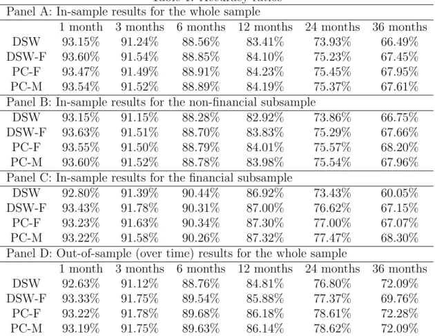
A good credit risk model should also be useful in discriminating good credits from bad ones. A common measure of this is accuracy ratio, the area between the power curve of a given model and the power curve of totally uninformative default predictions over the sim-ilar area defined by a perfect ranking model and totally uninformative default predictions. Both the power curve and the accuracy ratio are ordinal measures. They only depend on the rankings implied by default probabilities, not on their absolute magnitudes. A detailed description can be found in Crosbie and Bohn (2002). To examine our models’ in-sample performance, we estimate the cumulative default probabilities for each firm-month obser-vation employing the parameter values estimated on the full sample. Panel A of Table 1 reports the in-sample accuracy ratios for various prediction horizons – 1 month, 3 months, 6 months, 12 months, 24 months and 36 months.
As expected, the results for the DSW model are quite similar to the findings reported in DSW (2012). The predictions for short horizons are very accurate with the accuracy ratios for the 1-month and 3-month predictions exceeding 90%. The accuracy ratios for the 6-month and 12-month predictions are also very good with their values staying above 80%. As the horizon is increased to 24 months and 36 months, the accuracy ratios reduce to 73.93% and 66.49%, respectively. The other specifications perform similarly. However, one should note that the accuracy ratio is solely based on ordinal rankings and is also not able to discriminate between joint and separate defaults. Assessing a model’s performance needs to be complemented by other means as well.
We further examine the prediction accuracy using two sub-samples – financial and non-financial groups. Panels B and C of Table 1 report the results. The accuracy ratios for the non-financial sub-sample are quite close to those of the full sample. For the financial sub-sample, however, the DSW model has a markedly lower accuracy at longer horizons. Adding a frailty factor to the DSW model, i.e., DSW-F, obviously improves the prediction accuracy for financial firms. The two partially-conditioned forward-intensity models, PC-F
and PC-M, perform equally well as the DSW-F model in terms of the in-sample accuracy ratio analysis.
An out-of-sample analysis over time is also conducted, and the results are reported in Panel D of Table 1. Here, we estimate the models each month on an expanding window of data beginning at the end of 2000. We set the evaluation group to be the firm-months after the estimation window. For this out-of-sample accuracy ratio analysis, all models perform similarly.
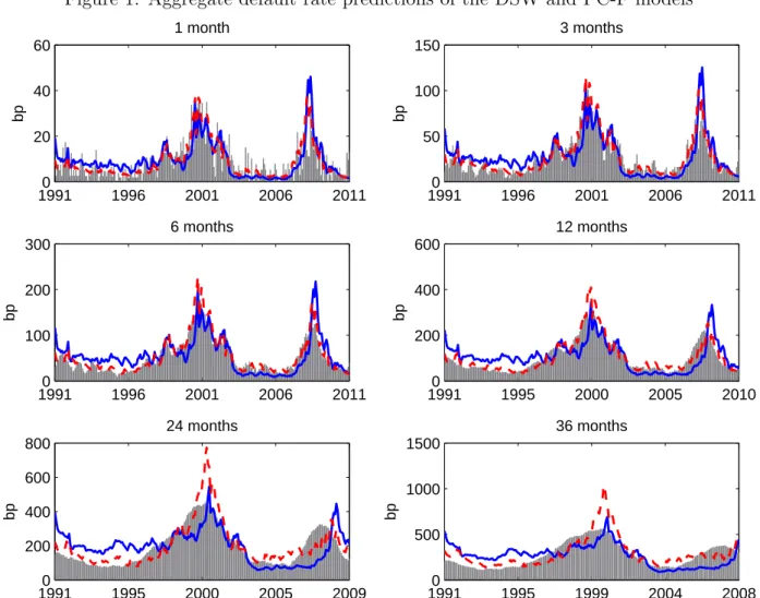
At each month-end, we compute the predicted rate of default for a prediction horizon among the active firms in the sample. We then compare it with the realized rate of default for the same group of firms in the intended prediction period. For each model, we repeat this for the entire sample period and for different prediction horizons: 1 month, 3 months, 6 months, 12 months, 24 months and 36 months.
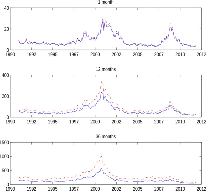
The bars in Figure 1 depict the realized rates of default for the intended prediction pe-riods. The DSW model’s results (solid curve) are basically same as the findings of DSW (2012), with a good performance at short horizons, but structural overestimation (underesti-mation) of default rates at the beginning (end) of the sample at longer horizons. In contrast, all other specifications with the frailty factor, go a long way in correcting the biases. The usefulness of a frailty factor in capturing common variation missed by the observable covari-ates is in line with the findings of Duffie, et al (2009) and Koopman, et al (2009). In Figure 1, we only present the results for the PC-M model (dashed curve), which is the best among the three specifications with the frailty factor. The model parameter values for both the DSW and PC-M models are in-sample, i.e., estimated using the whole sample. As Figure 1 shows, conditioning the forward intensities on a common risk factor such as frailty is very important in correcting prediction biases for longer horizons.
4.5
Parameter estimates
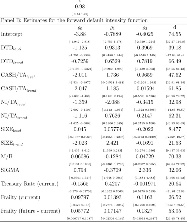
In the following discussion, we focus on the parameter estimates of the PC-F model. The results for the PC-M model are qualitatively similar. Panel A of Table 2 presents the param-eter governing the frailty dynamics, suggesting high persistence with c = 0.99. Panel B of Table 2 reports the parameter estimates and confidence intervals of the partially-conditioned default intensity function. The parameter estimates and confidence intervals for the other-exits intensity function are given in Table 3. Note that in this study, the other-other-exits intensity function remains the same regardless of the model for the default intensity.
The Nelson-Siegel parameters by themselves are somewhat difficult to interpret. Thus, we report in Figures 2 and 3 the implied term structures for the coefficients in the default
in-tensity functions for the firm-specific and common risk factors as well as their 90% confidence bands.
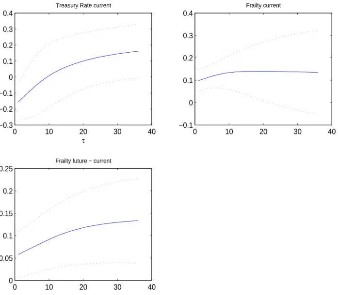
The patterns exhibited by the coefficients for the firm-specific attributes in Figure 2 are largely similar to those of of DSW (2012), and readers are referred to that paper for compar-ison. An important difference is that our inference is more conservative (wider confidence bands) by allowing unrestricted cross-sectional correlations in our pseudo-scores. Still, the coefficients on the firm-specific attributes remain fairly well identified. The situation changes for the common risk factors reported in Figure 3. The confidence bands are much wider than is the case for the macro variables in DSW (2012). This is likely due to our more conservative but more appropriate way of approaching the statistical inference. Similarly to DSW (2012), we find that coefficient of the 3-month Treasury bill rate switches signs. The current value of the frailty factor has a roughly constant effect on the forward intensities across the maturity spectrum, whereas the additional effect of the future path of the frailty factor increases with maturity.
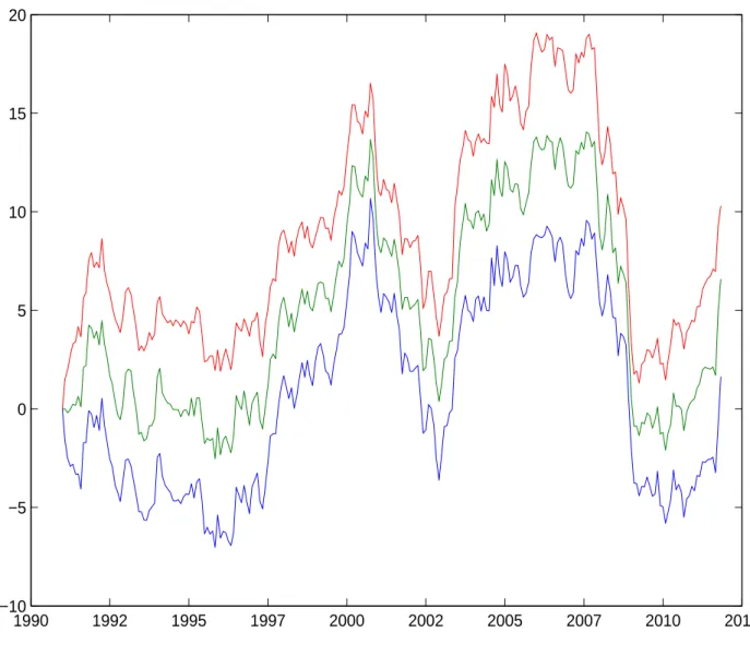
Figure 4 depicts the path of the filtered values for the frailty factor, using the particle filter computed at the full-sample parameter estimates. We observe positive frailty values in the default waves before 2008, signaling that variation of the observable covariates is insufficient to fully explain the default cycles. Similar to what have been found in Koopman, et al (2009), the frailty factor takes up negative values during the recent financial crisis, reflecting fewer than the expected number of defaults given the value of the observable covariates. Hence, the frailty factor is likely to have taken up the role of the bail-out dummy variable of DSW (2012) to capture the massive government intervention post-Lehman Brothers’ bankruptcy.
4.6
Portfolio default distributions
Allowing correlations among individual forward default intensities is of the first-order impor-tance when one is interested in the joint behavior of defaults. In this subsection, we use the PC-F model to illustrate this point. The PC-M model by partially-conditioning on future value of interest-rates can also produce similar results.
Figure 5 reports the difference in the log-pseudo-likelihoods at different time points be-tween the PC-F and DSW models. In contrast to the measures examined earlier, these log-pseudo-likelihoods reflect the goodness-of-fit of the different specifications on the whole portfolio. One can clearly see that the PC-F model easily beats the DSW model throughout the entire sample period. Its superiority is especially clear at the beginning of the sample period and during the default waves. We note that using the results in Vuong (1989) we could form a formal statistical test based on the full-sample log-pseudo-likelihood difference.
However, the Wald test on the parameter restrictions can be more easily conducted with the self-normalized approach described in Appendix.4
Next, we investigate the consequences of forward default correlations on the distribution for the number of defaults in the portfolio. We use a conditional Monte-Carlo simulation technique to compute the default distribution under the PC-F model. Specifically, we first simulate paths of the common factors, and on each simulated path, we compute the exact conditional distribution for the number of defaults using the convolution algorithm given in Duan (2010). The unconditional default distribution then follows by averaging the con-ditional probabilities. To flush out the effect of default correlations, we also compute the individual default probabilities under the same model, and construct a version of the distri-bution for the number of defaults by assuming no forward default correlation.
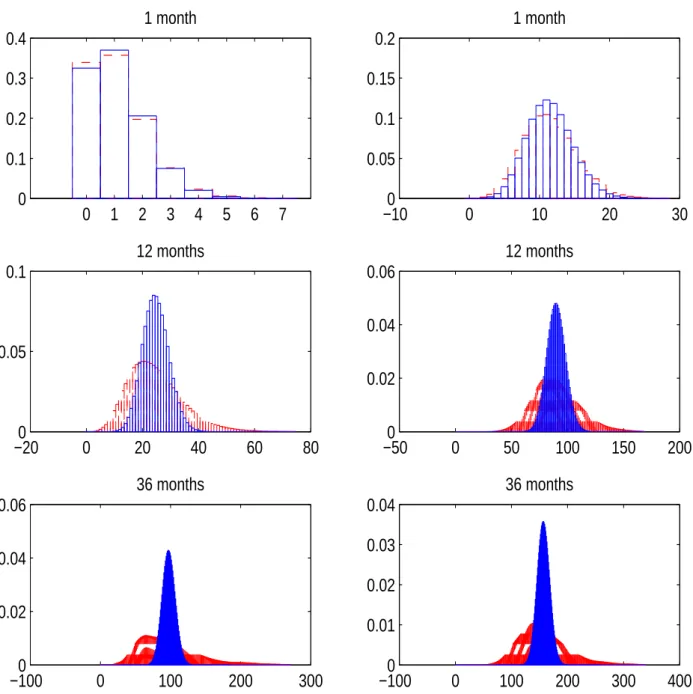
Figure 6 reports these two distributions at two dates for three prediction horizons. The left column shows the predictions in May 2007, before the blow-up of the BNP hedge funds which was one of the first signs of the financial crisis. The right column reports the predictions in October 2008, the month after Lehman Brothers’ bankruptcy. One can see in the top panel (one-month prediction horizon) that the distributions for the two dates are very different, with the one after the bankruptcy of Lehman Brothers being much closer to normality. The intuition is that much higher individual default probabilities allow the Central Limit Theorem to kick in faster to exhibit an approximate normality, whereas lower individual default probabilities make no default a more likely event and hence the portfolio default distribution exhibits a truncated look. Note also that the portfolio default distributions under two modeling assumptions are very similar. Forward default correlations has a rather minor effect simply because correlations in this case solely come from the latency of the frailty factor. The future value of the partial conditioning variable (i.e., the frailty factor in the PC-F model) cannot play any role for the one-month prediction horizon (i.e., τ = 0).
A sharp contrast can be seen in the middle panel for the 12-month prediction horizon where the two portfolio default distributions show a large difference. The one under the PC-F model without assuming away default correlations shows heavy tails. Forward default correlations arising from partial conditioning obviously make the default distribution much more spread out. Furthermore, the shape of the distribution is also changed. Under the conditional independence assumption, the number of defaults is symmetric and is fairly close to being normally distributed. Once forward default correlations are properly accounted for, a more skewed and heavy-tailed distribution emerges. This result is due to mixing different
4The quantities that would be needed for the likelihood-based tests are the inverse Hessian and an estimate
of the variance of the scores. The former is available from our algorithm (see Appendix) whereas the latter would need to be estimated by a HAC-type approach. Given strong dependence in the scores from the use of overlapping data points, we feel that invoking the usual consistency argument for the resulting variance estimator may be problematic.
conditional default distributions over the random future paths of the common factor (i.e., the frailty factor in the PC-F model). The bottom panel suggests that the effect of forward default correlations becomes even stronger when the prediction horizon is increased to 36 months.
To show that these results are not specific to a given date, Figure 7 presents the 99th percentile of the portfolio default distribution, with and without forward default correlations, over the sample period. The upper tail of the portfolio default distribution is of particu-lar interest to risk management (e.g., computing credit VaRs) and the rating and pricing of structured finance instruments like senior CDO tranches. Not surprisingly, Figure 7 suggests that ignoring forward default correlations as in the DSW model can lead to a severe underes-timation of the upper tail of the portfolio default distribution. A novel and interesting result conveyed by the plots in Figures 6 and 7 is that the effect of forward default correlations becomes more pronounced when the prediction horizon is increased. Since structured debts may have fairly long maturities, say 5 years, the issue of default correlations should not be taken lightly.
5
Appendix
5.1
Handling the latent frailty factor: particle filtering
As the frailty factor is unobserved, we need a filter to compute conditional expectations. We use the smooth particle filter of Malik and Pitt (2011) to sample from the filtering distribution
f (Fj∆t|Dj∆t) where Dj∆t is the information set at j∆t. To understand the algorithm, first
consider the the following theoretical recursion:
f (Fj∆t|Dj∆t)∝ f(Fj∆t|F(j−1)∆t) ( N ∏ i=1 Pi,j,0(Y(j−1)∆t, F(j−1)∆t) ) f (F(j−1)∆t|D(j−1)∆t) (21)
that follows from Bayes’ rule and conditional independence of the one-period exit proba-bilities. Here, the one-period probabilities, Pi,j,0(Y(j−1)∆t, F(j−1)∆t), are defined by equation
(16).
Also note the fact that the defaults in period j∆t only depend on the frailty in period (j− 1)∆t, a result of our assumption that the variables are observed at the end of a given month (for instance, default in February depends on the value of the macro variables and frailty at the end of January).
This equation can then be implemented using sequential importance sampling with re-sampling. In particular, assume that we have M particles representing f (F(j−1)∆t|D(j−1)∆t),
1. Attach importance weights wj∆t(m) to the particles w(m)j∆t = N ∏ i=1 Pi,j,0(Y(j−1)∆t, F (m) (j−1)∆t).
2. Resample the particles with weights proportional to wj∆t(m) using the smooth bootstrap sampling technique of Malik and Pitt (2011).
3. Sample from the transition density
Fj∆t(m) ∼ f(Fj∆t|F (m) (j−1)∆t).
The resulting particle cloud, Fj∆t(m)for m = 1,· · · , M, approximately represents f(Fj∆t|Fj∆t).
Then, to obtain the expectations over the path of the common variables ˜Zj∆t:j∆t+τ, we
sim-ulate M paths. To decrease Monte Carlo noise, we use the same random numbers for calls at different parameter values.
5.2
Parameter estimation by Sequential Monte Carlo (SMC)
Lack of decomposability means that the number of parameters to be estimated jointly will be very large. The conventional gradient-based optimization methods will not work well and statistical inference becomes challenging. Fortunately, a pseudo-Bayesian device can be used for estimation and inference under our model. Consider the following pseudo-posterior distribution: γt(θ) ∝ t ∏ j=0 Lj,min(T−j∆t,τ)(θ)π(θ), for t = 1,· · · , T ∆t− 1 (22)
and apply the sequential batch-resampling routine of Chopin (2002) together with tempering steps as in Del Moral, et al (2006). For each t, this procedure yields a weighted sample of
N points, (θ(i,t), w(i,t)) for i = 1,· · · , N, whose empirical distribution function will converge to γt(θ) as N increases. In what follows, the superscript i is for i = 1,· · · , N.
Initialization : Draw an initial random sample from the prior: (θ(i,0) ∼ π(θ), w(i,0) = 1 N)
Here, the only role of the prior, π(θ), is to provide the initial particle cloud from which the algorithm can start. Of course, the support of π(θ) must contain the true parameter value
θ0.
Recursions and defining the tempering sequence: Assume we have a particle cloud
(θ(i,t), w(i,t)) whose empirical distribution represents γ
t(θ). Then, we will arrive at a cloud
moving directly from γt(θ) to γt+1(θ) is too ambitious as the two distributions are too far
from each other. This will be reflected in highly variable importance weights if one resorts to direct importance sampling. Hence, following Del Moral, et al (2006), we build a tempered bridge between the two densities and evolve our particles through the resulting sequence of densities. In particular, assume that at t + 1, we have Pt+1 intermediate densities:
¯
γt+1,p(θ)∝ γt(θ)L ξp
t+1,min(T−(t+1)∆t,τ)(θ) (23)
This construction defines an appropriate bridge: when ξ0 = 0, ¯γt+1,0(θ) = γt(θ), and when
ξPt+1 = 1, ¯γt+1,Pt+1(θ) = γt+1(θ). We can initialize a particle cloud representing ¯γt+1,0(θ) as
(¯θ(i,t+1,0) = θ(i,t), ¯w(i,t+1,0) = w(i,t)). Then, for p = 1, . . . , Pt+1 we move through the sequence
as follows.
• Reweighting Step: In order to arrive at a representation of ¯γt+1,p(θ) we can simply
use the particles representing ¯γt+1,p−1(θ) and the importance sampling principle. This
leads to ¯ w(i,t+1,p) = w¯(i,t+1,p−1) γ¯t+1,p(¯θ (i,t+1,p)) ¯ γt+1,p−1(¯θ(i,t+1,p)) = ¯w(i,t+1,p−1)Lξp−ξp−1 t+1,min(T−(t+1)∆t,τ)(¯θ (i,t+1,p)) ¯ θ(i,t+1,p) = θ¯(i,t+1,p−1)
If one would keep on repeating the reweighting step, quickly all the weights would concentrate on a few particles, the well known phenomenon of particle impoverish-ment in sequential importance sampling. In the SMC literature, this is tackled by the resample-move step (see e.g Chopin (2002)). This is triggered whenever a measure of particle diversity, the efficient sample size, defined as ESS = (
∑N i=1w¯(i,t+1,p)) 2 ∑N i=1(w¯(i,t+1,p)) 2 falls
below a pre-defined constant, B. Here, resampling directs the particle cloud towards more likely areas of the sampling space, while move enriches particle diversity.
If ESS < B, perform the following resampling and move steps.
• Resampling Step: The particles are resampled proportional to their weights. If I(i,t+1,p) ∈
(1, . . . , N ) are particle indices sampled proportional to ¯w(i,t+1,p), the equally weighted
particles are obtained as ¯
w(i,t+1,p) = 1
N
¯
• Move Step: Each particle is passed through a Markov Kernel Kt+1,p(¯θ(i,t+1,p),·) that
leaves ¯γt+1,p(θ) invariant, typically a Metropolis-Hastings kernel:
1. Propose θ∗(i) ∼ Qt+1,p(· | ¯θ(i,t+1,p))
2. Compute the acceptance weight α = min (
1, ¯γt+1,p(θ∗(i))Qt+1,p(¯θ(i,t+1,p)|θ∗(i))
¯
γt+1,p(¯θ(i,t+1,p))Qt+1,p(θ∗(i)|¯θ(i,t+1,p))
) 3. With probability α, set ¯θ(i,t+1,p) = θ∗(i), otherwise keep the old particle
This step will enrich the support of the particle cloud while conserving its distribution. Importantly, given that we are in an importance sampling setup, the proposal distri-bution, Qt+1,p(· | ¯θ(i,t+1,p)), can be adapted using the existing particle cloud. In our
implementation, for instance, we use independent normal distribution proposals that are fitted to the particle cloud before the move. To improve the support of the particle cloud further, one can execute multiple such M-H steps each time.
When p = Pt+1is reached, we obtain a representation of γt+1(θ) as (θ(i,t+1) = ¯θ(i,t+1,Pt+1),
w(i,t+1) = ¯w(i,t+1,Pt+1)). Following Del Moral, et al (2011), we set the tempering
se-quence ξp automatically to ensure that the efficient sample size stays close to B. We
achieve this by a grid search, where we evaluate the ESS at a grid of candidate ξp and
then settle with the one that produces the closest ESS to B.
Pre-Estimated Macro Dynamics: It is important to point out an additional
compli-cation when the future path of some macro-variables is part of the conditioning set. As suggested in Section 4.3, the parameters of the macro-dynamics are estimated in a prelim-inary run, separately from the SMC procedure. Further, to properly conduct inference as described in the next section, we need an expanding data structure for all the parameter estimates. Hence, when moving from t to t + 1, the point estimate for the parameter of the macro-dynamics changes from ˆθM
t to ˆθMt+1. Then, for all j ≤ t + 1, the pseudo-likelihoods
change from Lj,min(T−j∆t,τ)(θ| ˆθMt ) to Lj,min(T−j∆t,τ)(θ| ˆθMt+1). To accommodate this change,
the following approach is used:
• First, the parameters of the macro-dynamics are kept fixed at ˆθM
t and the algorithm
described above allows us to obtain a representation of
t+1∏ j=0
Lj,min(T−j∆t,τ)(θ| ˆθtM)π(θ).
• Then, the new macro-parameter, ˆθM
t+1 is computed. We obtain a representation of
the new target,
t+1∏ j=0
Lj,min(T−j∆t,τ)(θ | ˆθMt+1)π(θ), by multiplying the weight: winc =
t+1∏ j=0 Lj,min(T−j∆t,τ)(θ|ˆθt+1M ) t+1∏ j=0 Lj,min(T−j∆t,τ)(θ|ˆθtM) .
5.3
Inference
Denote the pseudo-posterior mean of the parameter by ˆθt:
ˆ θt = 1 ∑N i=1w(i,t) N ∑ i=1 w(i,t)θ(i,t)
γt(θ) is not a true posterior because the likelihood function in equation (24) is not a true
likelihood function. Thus, it cannot directly provide valid Bayesian inference. However, we can turn to the results of Chernozhukov and Hong (2003) to give a classical inter-pretation to our simulation outcome. In particular, denote the log-pseudo posterior by
lt(θ) = t
∑
j=0
ln Lj,τ(θ) + ln π(θ). Let the pseudo-score matrix be st(θ) =∇θlt(θ) and the
nega-tive of the scaled Hessian be Jt(θ) =−∇θθ′lt(θ)/t. Then, Theorem 1 of Chernozhukov and
Hong (2003) states that for large t, γt(θ) is approximately a normal density with the random
mean parameter: θ0+ Jt(θ0)−1st(θ0)/t. This result implies that the pseudo posterior mean
ˆ
θt provides a consistent estimate for θ0, and the scaled estimation error can be characterized
by √
t(ˆθt− θ0)≈ Jt(θ0)−1st(θ0)/
√
t (24)
In addition to consistency, asymptotic normality follows by applying the Central Limit Theorem (CLT) to the scores. Chernozhukov and Hong (2003) showed that asymptotically, the covariance matrix of the pseudo-scores is equal to the inverse Hessian, Jt(θ0)−1, hence
the latter can be estimated by the former. In turn, the variance of the scores could be estimated by its empirical counterpart. All this would allow us to construct the sandwich matrix necessary for inference.
However, access to the recursive estimates ˆθt provides us a more direct way to construct
the confidence band using the self-normalized approach of Shao (2010). Thus, we can bypass the delicate issue of estimating asymptotic variance. Knowing that the pseudo-score is asymptotically normal, we assume that the functional CLT applies to the scaled pseudo-score: Jt(θ0)−1 1 √ ts[rt](θ0)→ d SW k(r), r∈ [0, 1] (25)
where S is an unknown lower triangular matrix, k is the number of parameter, and Wk(r) is
a k-dimensional Brownian motion.
Following Shao (2010), we define a norming matrix ˆ Ct= 1 t2 t ∑ l=1 l2(ˆθl− ˆθt)(ˆθl− ˆθt)′ (26)
Then, we can form the following asymptotically pivotal statistic
t(ˆθt− θ0) ˆCt−1(ˆθt− θ0)′ →d Wk(1)Pk(1)−1Wk(1) (27)
where the asymptotic random norming matrix Pk(1) =
∫1
0(Wk(r)−rWk(1))(Wk(r)−rWk(1))′dr
is a path functional of the Brownian bridge. The main insight is that the nuisance scale ma-trix S disappears from this quadratic form, and thus it need not be estimated.
The above result can be used to form tests. For example, we can test the hypothesis of the i -th element of θ0, denoted by θ
(i)
0 , equal to a by the following robust analogue to the
t-test: t∗ = ˆ θ(i)T /∆t−1− a √ ˆ δi,T /∆t−1 →d W (1) [∫1 0(W (r)− rW (1))2dr ]1/2 (28)
where ˆδi,T /∆t−1 is the ith diagonal element of ˆCT /∆t−1. The right-hand-side random variable
does not have a known distribution, but can be easily simulated. Kiefer, et al (2000) reported that the 95% quantile is 5.374 and the 97.5% quantile is 6.811. These values can also be used to set up confidence intervals.
We would like to point out a particular strength of our inference procedure. It does not require an explicit computation of the individual scores or the Hessian, and hence can be seamlessly extended to non-smooth objective functions without any extra work. In our case, specifications with multi-dimensional frailty factors (e.g., to allow for industry-level frailties as in Koopman, et al (2009)) would constitute such an example, because the smooth particle filter of Malik and Pitt (2011) only works for one-dimensional latency. In general, our combination of recursive parameter estimation and self-normalized inference is likely to be useful for the analysis of any dynamic model with a particle filter and involving pseudo-likelihoods. An alternative approach for such cases will be to use the sandwich matrix and to compute the scores using the marginalized score method advocated in Doucet and Shephard (2012).
5.4
Real-time updating
In reality, portfolio credit risk models need to be updated periodically as new data arrive and/or some old data get revised. In our notation, this would mean that the final date T is increased to T + 1. Note that for the ease of exposition, T in this section denotes the number of periods as opposed to the length of time used earlier. A particular strength of our methodology is that the estimation routine does not need to be re-initialized from the prior as the pseudo-posterior using data up to T will provide a much better proposal distribution.
Let the pseudo-posterior at T be denoted by
γTT(θ)∝
T∏−1 j=0
LTj,min((T−j)∆t,τ)(θ)π(θ)
whereas the pseudo-posterior at T + 1 by
γT +1T +1(θ)∝
T
∏
j=0
LT +1j,min((T +1−j)∆t,τ)(θ)π(θ)
The superscript is introduced to differentiate the pseudo likelihoods at T and T + 1. Due to data revisions, for example, it may be the case that LT +1j,k (θ) ̸= LT
j,k(θ).
Assume that from the previous run up to T we have a weighted set of particles (θ(i,T ), w(i,T ))
representing the pseudo-posterior γT
T(θ). Next, set θ(i,T +1)= θ(i,T ) and reweight by
w(i,T +1) = w(i,T )×γ T +1 T +1(θ (i,T +1)) γT T(θ(i,T +1)) (29) Since the denominator is already available from the previous run, one only needs to compute the numerator using the new and revised data set. Then, the weighted set (θ(i,T +1), w(i,T +1)) represents the new pseudo-posterior γT +1T +1(θ). If the weights are too uneven, intermediate tempered densities can be constructed and resample-move steps similar to those in Section 5.2 can be executed.
References
[1] Altman, E., 1968, Financial Ratios, Discriminant Analysis and the Prediction of Corpo-rate Bankruptcy, Journal of Finance 23, 589–609.
[2] Beaver, W., 1966, Financial Ratios as Predictors of Failure, Journal of Accounting
Re-search 4, 71–111.
[3] Bharath, S. T., and T. Shumway, 2008, Forecasting Default with the Merton Distance to Default Model, Review of Financial Studies 21, 1339–1369.
[4] Campbell, J. Y., J. Hilscher, and J. Szilagyi, 2008, In Search of Distress Risk, Journal of
Finance 63, 2899–2939.
[5] Chava, Sudheer, and Robert A. Jarrow, 2004, Bankruptcy Prediction with Industry Effects, Review of Finance 8, 537–569.
[6] Chernozhukov, V. and Hong, H., 2003, An MCMC Approach to Classical Estimation,
Journal of Econometrics 115, 293–346.
[7] Chopin, N., 2002, A Sequential Particle Filter Method for Static Models, Biometrika 89, 539–551.
[8] Crosbie, P., and J. Bohn, 2002, Modeling Default Risk, technical report, KMV LLC. [9] Del Moral P, Doucet A, Jasra A (2006) Sequential Monte Carlo Samplers, Journal of
Royal Statistical Society B 68, 411–436.
[10] Del Moral P, Doucet A, Jasra A (2011) An Adaptive Sequential Monte Carlo Method for Approximate Bayesian Computation. Statistics and Computing, DOI: 10.1007/s11222-011-9271-y.
[11] Doucet A, and Shephard N (2012) Robust Inference on Parameters via Particle Filters and Sandwich Covariance Matrices, working paper, Oxford-Man Institute, University of Oxford.
[12] Duan, J. C., 2010, Clustered Defaults, National University of Singapore working paper. [13] Duan, J.C., Sun, J. and T. Wang, 2012, Multiperiod Corporate Default Prediction - A
Forward Intensity Approach, Journal of Econometrics 170, 191–209.
[14] Duffie, D., A. Eckner, G. Horel and L. Saita, 2009, Frailty Correlated Default, Journal
[15] Duffie, D., L. Saita, and K. Wang, 2007, Multi-period Corporate Default Prediction with Stochastic Covariates, Journal of Financial Economics 83, 635–665.
[16] Kiefer, N. M., Vogelsang, T. J. and Bunzel, H., 2000, Simple Robust Testing of Regres-sion Hypotheses. Econometrica 68, 695-714
[17] Koopman, S.J., A. Lucas, and B. Shwaab, 2009, Macro, Industry and Frailty Effects in Defaults: The 2008 Credit Crisis in Perspective, forthcoming in Journal of Business and
Economic Statistics (2013).
[18] Malik, S., and M. K. Pitt, 2011, Particle Filters for Continuous Likelihood Evaluation and Maximisation, Journal of Econometrics 165, 190–209.
[19] Shao, X., 2010, A Self-Normalized Approach to Confidence Interval Construction in Time Series. Journal of the Royal Statistical Society: Series B 72, 343–366.
[20] Shumway, T., 2001, Forecasting Bankruptcy More Accurately: A Simple Hazard Model,
Journal of Business 74, 101–124.
[21] Vuong, Q.H, 1989, Likelihood Ratio Tests for Model Selection and Non-nested Hypothe-ses, Econometrica 57, 307–333.
Figure 1: Aggregate default rate predictions of the DSW and PC-F models 19910 1996 2001 2006 2011 20 40 60 1 month bp 19910 1996 2001 2006 2011 50 100 150 3 months bp 19910 1996 2001 2006 2011 100 200 300 6 months bp 19910 1995 2000 2005 2010 200 400 600 12 months bp 19910 1995 2000 2005 2009 200 400 600 800 24 months bp 19910 1995 1999 2004 2008 500 1000 1500 36 months bp
This figure presents the predicted default rates for two models: DSW (solid blue curve) and PC-F (dashed red curve). Realized default rates are the gray bars.
Figure 2: Parameter estimates for the firm-specific attributes in the forward default intensity function of the PC-F model
0 20 40 −6 −4 −2 Intercept τ 0 20 40 −2 −1 0 DTDlevel τ 0 20 40 −1 −0.5 0 DTDtrend τ 0 20 40 −4 −2 0 CASH/TAlevel τ 0 20 40 −3 −2 −1 CASH/TAtrend τ 0 20 40 −4 −2 0 NI/TAlevel τ 0 20 40 −2 −1 0 NI/TAtrend τ 0 20 40 −0.2 0 0.2 SIZElevel τ 0 20 40 −5 0 5 SIZEtrend τ 0 20 40 −0.2 0 0.2 M/B τ 0 20 40 −2 0 2 SIGMA τ
This figure shows the parameter estimates for the forward default intensity function corresponding to different prediction horizons under the PC-F model. DTD is the distance to default, CASH/TA is the sum of cash and short-term investments over the total assets, NI/TA is the net income over the total assets, SIZE is log of firm’s market equity over the average market equity value of the S&P500 company, M/B is the market to book equity value ratio, SIGMA is the 1-year idiosyncratic volatility. The subscript “level” denotes the average in the preceding 12 months, “trend” denotes the difference between its current value and the preceding 12-month average. The solid blue curve is for the parameter estimates and the dotted red curves depict the 90% confidence interval.
Figure 3: Parameter estimates for the common risk factors in the forward default intensity function of the PC-F model
0 10 20 30 40 −0.3 −0.2 −0.1 0 0.1 0.2 0.3 0.4
Treasury Rate current
τ 0 10 20 30 40 −0.1 0 0.1 0.2 0.3 0.4 Frailty current 0 10 20 30 40 0 0.05 0.1 0.15 0.2 0.25
Frailty future − current
This figure shows the parameter estimates for the forward default intensity function corresponding to different prediction horizons under the PC-F model.“Treasury Rate” is the 3-month US Treasury rate, “Frailty” is the common latent factor. The solid blue curve is for the parameter estimates and the dotted red curves depict the 90% confidence interval.
Figure 4: Estimates of the frailty factor time series under the PC-F model 1990 1992 1995 1997 2000 2002 2005 2007 2010 2012 −10 −5 0 5 10 15 20
This figure shows the 5, 50 and 95 % quantiles of the filtered frailty factor under the PC-F model. The frailty factor is obtained by applying the full-sample parameter estimates to the particle filter.
Figure 5: Log-pseudo-likelihood differences between the PC-F and DSW models 1990 1992 1995 1997 2000 2002 2005 2007 2010 2012 −10 0 10 20 30 40 50 60 70 80
Figure 6: Portfolio default distributions implied by the PC-F model with and without default correlations under two market conditions
0 1 2 3 4 5 6 7 0 0.1 0.2 0.3 0.4 1 month −100 0 10 20 30 0.05 0.1 0.15 0.2 1 month −200 0 20 40 60 80 0.05 0.1 12 months −500 0 50 100 150 200 0.02 0.04 0.06 12 months −1000 0 100 200 300 0.02 0.04 0.06 36 months −1000 0 100 200 300 400 0.01 0.02 0.03 0.04 36 months
This figure shows the distribution for the number of defaults in the full population implied by the two models at two different dates. The dotted histogram depicts the distribution implied by the PC-F model, whereas the solid histogram is the distribution when default correlations are ignored. The left column shows the predicted distributions in May 2007, before the onset of financial crisis, whereas the right column is for the distributions in October 2008, after Lehman Brothers’ bankruptcy. The top panel shows the results for the


![Table 3: Estimates for the forward other-exits intensity function ϱ 0 ϱ 1 ϱ 2 d Intercept -3.951 1.045 0.6421 55.27 [-4.536 -3.366] [-0.7154 2.806] [-0.6826 1.967] [37.29 73.25] DTD level 0.03655 -0.09309 -0.03917 20.8 [-0.03562 0.1087] [-0.1984 0.01219] [](https://thumb-eu.123doks.com/thumbv2/123dok_br/18233545.878270/36.892.163.761.221.769/table-estimates-forward-exits-intensity-function-intercept-level.webp)
