ESTIMATE OF STAND DENSITY INDEX FOR EUCALYPTUS UROPHYLLA
USING DIFFERENT FIT METHODS
1Ernani Lopes Possato2*, Natalino Calegario3, Gilciano Saraiva Nogueira4, Elliezer de Almeida Melo2 and Joyce de Almeida Alves2
1 Received on 21.01.2014 accepted for publication on 16.09.2016.
2 Universidade Federal de Lavras, Programa de Pós-Graduação em Engenharia Florestal, Lavras, MG - Brasil. E-mail: <[email protected]>, <[email protected]> and <[email protected]>.
3 Universidade Federal de Lavras, Departamento de Ciências Florestais, Lavras, MG - Brasil. E-mail: <[email protected]>. 4 Universidade Federal dos Vales do Jequitinhonha e Mucuri - Campus JK, Faculdade de Ciências Agrária, Departamento de Engenharia Florestal, Diamantina, MG - Brasil. E-mail: <[email protected]>.
*Corresponding author.
ABSTRACT – The Reineke stand density index (SDI) was created on 1933 and remains as target of researches due to its importance on helping decision making regarding the management of population density. Part of such works is focused on the manner by which plots were selected and methods for the fit of Reineke model parameters in order to improve the definition of SDI value for the genetic material evaluated. The present study aimed to estimate the SDI value for Eucalyptus urophylla using the Reineke model fitted by the method of linear regression (LR) and stochastic frontier analysis (SFA). The database containing pairs of data number of stems per hectare (N) and mean quadratic diameter (Dq) was selected in three intensities, containing the 8, 30 and 43 plots of greatest density, and models were fitted by LR and SFA on each selected intensities. The intensity of data selection altered slightly the estimates of parameters and SDI when comparing the fits of each method. On the other hand, the adjust method influenced the mean estimated values of slope and SDI, which corresponded to -1.863 and 740 for LR and -1.582 and 810 for SFA.
Keywords: Reineke Index; Stochastic Frontier Analysis; Linear Regression
ESTIMATIVA DO ÍNDICE DE DENSIDADE DO POVOAMENTO PARA
EUCALYPTUS UROPHYLLA UTILIZANDO DIFERENTES MÉTODOS DE
AJUSTES
RESUMO – O índice de densidade do povoamento (IDP) de Reineke, concebido na década de 1930, continuou sendo objeto de pesquisas em razão de sua importância no auxílio de tomada de decisões relacionadas à condução da densidade de um povoamento. Parte destes trabalhos se concentra na forma de seleção de parcelas e em métodos de ajuste dos parâmetros do modelo de Reineke, visando aprimorar a definição do valor do IDP para o material genético avaliado. Objetivou-se neste estudo estimar o valor do IDP, para Eucalyptus urophylla, utilizando o modelo de Reineke, ajustado pelo método de regressão linear (RL) e pela análise de fronteira estocástica (AFE). A base de dados, contendo os pares de dados número de fustes por hectare (N) e diâmetro quadrático médio (Dq), foi selecionada em três intensidades, contendo 8, 30 e 43 parcelas de maior densidade, sendo em cada uma delas realizados os ajustes do modelo pelos diferentes métodos. A intensidade de seleção dos dados pouco alterou as estimativas dos valores dos parâmetros do modelo e do IDP, entre os ajustes de cada método. Por outro lado, o método de ajuste influenciou nos valores médios estimados da inclinação da reta e do IDP sendo iguais a, respectivamente, -1,863 e 740, para RL, -1,582 e 810, para AFE.
1. INTRODUCTION
The importance to know the growth, dynamics of canopy, mortality of trees, among other aspects interesting to the manager are strongly associated to the number of trees and their dimensions, especially their diameter. In this sense the use of Stand Density Index is common, which reflects quantitatively the degree of trees occupation of a given area, what may be directly associated to the growth of each individual and the population as a whole (AVERY; BURKHART, 1994). The self-thinning law (YODA et al., 1963), which evaluates the relationship between biomass and number of individuals per unit of area, and also the stand density index (SDI) proposed by Reineke (1933) based on the relationship between the number of stems per area (N) and mean quadratic diameter (Dq) stand out among the works regarding density of trees. The last author observed that the shape of maximum density curve in even-aged stands is the same, independently of their age, site or plantation density, and among different species the slope (considering the logarithmic base (Ln)) was -1.605, with differences only on the intercept, k (1).
Ln(N) = k – 1.605Ln(Dq)
According to Reineke (1933), the SDI consists on the maximum number of trees per unit of area in which the stand Dq is equal to 10 inches or 25.4 cm. Thus, when isolating k and substituting in (1), one finds (2):
Ln(SDI) = k – 1.605Ln(25.4):. Ln(SDI) =
Ln(N) +1.605Ln
Therefore, SDI represents a measurement of density based on the two components of basal area – number of stems per hectare and mean quadratic diameter (AVERY; BURKHART, 1994). Since it was created, many researchers endeavored to validate or improve the estimate of SDI value, or even to attest the independency of factors like age and productive capacity (BREDENKAMP; BURKHART, 1990; TANG et al., 1994; ZEIDE, 1995; PRETZSCH; BIBER, 2005). Other aspect mentioned when estimating the SDI value of a given species is the database used for this purpose. The insistence to validate the density indices exists in function of the need for an accurate estimate of its value, since its use may influence the management of a stand density.
Considering that the index deals with a maximum limit, one of the principles that must be considered on determining the SDI is the selection of database for the model fit. According to Reineke (1933), the data used (N and Dq) must came from measurements of fully stocked stands, it means, in a situation of intense competition, and then the fit will lead to a slope of -1.605, as recommended by the author.
Since the density involves at least two variables, N and Dq, the selection of plots in a scenario of high competition is not a trivial task. A stand may be in high competition when the Dq value is low and N is high, as well as in situations of low N and high Dq, or in conditions of intermediate values of such variables. Furthermore, one may consider the subjectivity to define when a stand may be considered close to the limit of maximum competition in relation to the pairs N and Dq.
Other important issue was defined by Weller (1990), who distinguished two types of self-thinning limit line: static and dynamics. Despite the study considers the self-thinning law, its theory is applicable to the Reineke model. The static limit is related to the maximum possible density supported by a given species and the dynamic limit represents the maximum of a determined studied stand, which in many cases is inferior to the static limit of that species. One of the reasons of the difference between the dynamic and static limits is the mortality caused by competition or not occur before the stand attain the maximum line of density (del RÍO et al; BRAVO, 2001).
Several methods for selection of plots were used in studies involving the SDI, for example, relative density (DREW; FLEWELLING, 1979; MEYER et al., 2013; SOLOMON; ZHANG, 2002), subdivision of Dq or N in classes (YANG; TITUS, 2002; ZHANG et al., 2005a), beginning of the occurrence of mortality when longitudinal data is available (HARVEY et al., 2011; del RÍO et al., 2001), among others.
On the other hand, some researches use different techniques to adjust the parameters of density models. The analysis of stochastic frontier, which has been used for years in economy, was evaluated in works estimating parameters of the self-thinning law model (BI et al., 2000; BI, 2004; ZHANG et al., 2005b).). This method was originally developed to estimate a function of productivity expressing the maximum production (1)
(2)
Dq 25.4 _____
of a given input in the productive process associated to a technological process (AIGNER et al., 1977). It estimates parameters of the line by decomposing the error in two components, what dispenses the manual intervention after fit, as made to determine the SDI by linear regression.
Studies involving SDI mostly use species of conifers as raw material. In the original work of Reineke (1933), only one species from 14, Eucalyptus globulus, belongs to the group of hardwoods. Such trend has been kept and nowadays there are few studies on the estimate of SDI for species of such group. Some exceptions were the works developed by Kumar, Long and Kumar (1995) with Tectona grandis and Bredenkamp and Burkhart (1990) with Eucalyptus grandis. The present work aimed to determine the limit of density in Eucalyptus urophylla stands (including its natural hybrids) by estimating the SDI considering different methods of fit of the Reineke model (linear regression and stochastic frontier analysis) in three intensities of plot selection.
2. MATERIAL AND METHODS 2.1. Database
Data were selected from inventories of Eucalyptus
urophylla even-aged stands (including its natural
hybrids) located on Western and Northern Goiás state, Brazil. Initially information on the number of stems per hectare (N), mean quadratic diameter (Dq) and stand age were selected from each sampling unit. Overall, 761 plots were selected containing only one measurement made on 2012 from stands implanted with the genetic material of interest.
The soil under the evaluated plantations is predominantly Red Latosol in both regions from where the data came from. The mean annual precipitation in Catalão is 1409 mm and 1522 in Niquelândia, with rains concentrated between October and March (GOIÁS, 2006). Plantations were implanted with different spacings, and the most common were 3.00 x 1.70 (37.8% of plots); 3.50 x 2.38 (18.6% of plots); 3.00 x 2.00 (17.7% of plots) and 3.00 x 1.50 (11.3% of plots). Other spacings were used (3.00 x 1.60; 3.50 x 1.70; 4.00 x 1.20; 4.00 x 1.5), but in only 14.6% of plots. The values ranged from 290 to 3753 for N, with means of 1295, from 8.0 to 24.9 cm for Dq, with means of 14.0 cm, and from 2.7 to 9.2 for age, with means of 5.7 years.
2.2. Selection of plots in competition
The preparation of data for the fit of SDI model started with the selection of plots under high competition. Thereunto, plots were subdivided into Dq classes with amplitude of 2.0 cm. Then, plots with more stems per hectare (N) on each class were selected in three intensities: Selection 1 (S1), in which only the plot with the highest N was selected on each Dq class; Selection 2 (S2), corresponding to the selection of four plots with the highest N on each class; Selection 3 (S3), which consisted on the six plots with highest N of each class. Then, three subsets were formed from the general database and the fit of Reineke model was conducted on each subset.
2.3. Determination of the stand density index value
The Reineke model (3) fitted by linear regression (LR) and stochastic frontier analysis (SFA) was used to determine the SDI of the genetic material
where Ln = neperian logarithm; N = number of stems per hectare; Dq = mean quadratic diameter (cm); = parameters of the equation; i = random error associated to the estimate of the i-th plot.
The fit of Equation (3) by LR was conducted using the method of ordinary least squares, which provides the fit of the mean line of data dispersion. In this method it was necessary to interfere manually in the fit to stablish the SDI of the species, since the line corresponds to the mean of plots in competition and not to the upper limit to them. Thereunto, the value of intercept fitted by regression was altered as the line passed by the plot with highest density, considering the pair of data N and Dq (4). In this case, the value of parameter 1 line slope fitted by LR was not altered.
where IDP = modified intersection parameter related to the maximum SDI; 1 = parameter related to the fitted line slope; Npi and Dqpi = values of N and Dq corresponding to the plot with highest density, which resulted in a higher IDP value.
The other method for fit was conducted by the stochastic frontier analysis. Such method dispenses the manual intervention to determine the intercept of maximum competition line, since parameters are fitted (3)
Ln(Ni) = 0 + 1Ln(Dqi)+i
as the line passes by the upper limit of data. Thereunto, the error (i) (3) is compounded by two random variables, i = vi + ui and both are independent and identically distributed (i.i.d) in relation to the data. The component
v assumes a normal distribution with means equal to zero and constant variance, N (0, ²), and is related to the error of random effect, while the second component of error (u) attends the condition of ui < 0, which in Econometrics is related to the technical and economic efficiency and presents asymmetric distribution (AIGNER et al.,1977).
The value 25.4 cm was considered to determine the SDI of the studied genetic material for each fit in the different selected database (S1, S2 and S3), with (5) for linear regression and (6) for stochastic frontier analysis.
The fit of SDI model by LR and SFA was conducted using the functions lm and sfa (package: frontier), respectively, contained in the software R (R DEVELOPMENT CORE TEAM, 2013).
2.4. Evaluation of fit methods
The methods used to adjust models were not compared in relation to the quality of fit. However, the estimated parameters were compared between themselves and also in relation to the value -1.605 recommended by Reineke (1933) by means of the determination of confidence interval (7).
in which 1 = estimated value of the parameter;
SE = standard error; DFres = degrees of freedom of residual; = reference value in the t distribution table for linear regression, and normal distribution for the function of stochastic frontier with á percent of significance in n-2 degrees of freedom. However, it is important to highlight that in this type of study the evaluation of fitted parameters is basically numeric, since the line slope was fixed by Reineke (1933) at -1.605, independently of the species, site or age of the stand. Therefore, the determination of confidence interval represents a statistical tool for the evaluation of the used methods of fit.
3. RESULTS
The presence of a density upper limit in the relationship between N and Dq was observed with negative exponential behavior and many individuals per hectare in lower values of Dq, thus reducing the N at each increase of Dq. Such reduction of N is strongly inclined next to the limit of density between 3500 and 2000 stems per hectare and Dq of until 15 cm, then reducing the decrease rate in lower densities of stems per hectare and Dq above this value. When the variables were transformed by the neperian logarithm, the relationship Ln(N)/Ln(Dq) assumed a decreasing linear behavior with the presence of a distinct upper limit corresponding to the limit of density (Figure 1).
The plots of database were distributed in nine classes of Dq, with the center of class ranging from 9.0 and 25.0 cm. The class with more plots were 15.0 cm (206 plots), followed by the class 13.0 (187 plots) and 17.0 cm (141 plots). In the class of 23.0 cm there were no plots, while the classes 21.0 and 25.0 cm contained only five and two sampling units, respectively. The other classes (9.0, 11.0 and 19.0 cm) contained respectively 55, 192 and 36 plots. Therefore, overall eight classes of Dq contained plots. Due to the reduced number of plots in the classes 21.0 and 25.cm, when four (S2) and six (S3) plots with the highest N were selected, eight plots were selected for S1, 30 for S2 and 43 for S3. The selected plots are illustrated on Figure 2 in logarithmic scale of N and Dq, and also a dashed line with slope of -1.605 used as illustrative reference of the line defined by Reineke (1933).
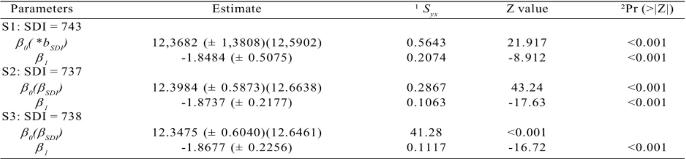
The presence of more disperse plots and distant from the density limit were observed in the selection of data S2 and S3 in lower classes, and mainly in those of highest Dq, when compared to plots of intermediate classes which are grouped and close to the limit (Figure 2). The parameters of Reineke model (3) fitted by LR were significant (p < 0.001), with â1 equal to -1.8484 (S1), -1.8737 (S2) and -1.8677 (S3) (Table 1) and statistically different from -1.605 (p < 0.05) when the equation was fitted using data S2 and S3. However, the values of slope did not differ (p < 0.05) among the fit in the three selection of plots, thus resulting in a total variation of only six stems per hectare among the SDI estimates, which corresponded to 743 (S1), 737 (S2) and 738 (S3) (Table 1).
(5) (6)
SDI = exp(SDI) 25.41
SDI = exp(0) 25.41
(7)
vDFres
SE < <
+
vDFres
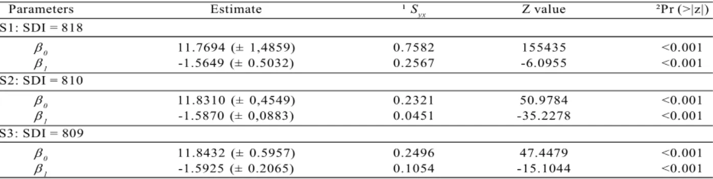
For the fit of Reineke model using SFA the parameters were significant (p < 0.001) for the three plot selections (Table 2). The values of line slope, -1.5649 (S1), -1.5870 (S2) and -1.5925 (S3), were numerically similar and statistically equal to the value of the original model of Reineke (-1.605) (p < 0.05). Similarly, to the fit by LR, the estimated values of SDI were little influenced by the data selection, varying in only nine stems per hectare, corresponding to 818 (S1), 810 (S2) and 809 (S3).
The mean values of intercept and slope were 12.633 and -1.863 for LR and 11.815 and -1.582 for SFA. Such means resulted in SDI of 740 for LR and 810 for SFA. Comparing the estimated values of parameters and SDI between the fit methods it is possible to observe that the slope was 0.2817 superior, it means, it presented a lower line slope, while the index was 70 stems per hectare higher by SFA than by LR.
Figure 1 – Relationship between number of stems per hectare (N) and quadratic mean diameter (Dq) in absolute values
and after transformation by natural logarithm (Ln).
Figura 1 – Relação entre número de fustes por hectare (N) e diâmetro quadrático médio (Dq), em valores absolutos e após transformação por logaritmo natural (Ln).
Figure 2 – Relationship between the number of stems per ha and quadratic mean diameter of the selection of one (S1), 4 (S2) and 6 (S3) plots by diameter class (dashed line: reference line with slope of -1.605).
Figura 2 – Relação entre o número de fustes por ha e diâmetro
quadrático médio da seleção de 1 (S1), 4 (S2) e 6 (S3) parcelas por classe de diâmetro (linha pontilhada: reta de referência com coeficiente angular de -1,605).
Table 1 – Estimates of parameters of Reineke model for each subset of data selected using linear regression as fit method.
Tabela 1 – Estimativas dos parâmetros do modelo de Reineke, para cada conjunto de dados selecionados, utilizando a regressão linear como método de ajuste.
Parameters Estimate ¹ Syx Z value ²Pr (>|Z|) S1: SDI = 743
0( *bSDI) 12,3682 (± 1,3808)(12,5902) 0.5643 21.917 <0.001
1 -1.8484 (± 0.5075) 0.2074 -8.912 <0.001 S2: SDI = 737
0(SDI) 12.3984 (± 0.5873)(12.6638) 0.2867 43.24 <0.001
1 -1.8737 (± 0.2177) 0.1063 -17.63 <0.001 S3: SDI = 738
0(SDI) 12.3475 (± 0.6040)(12.6461) 41.28 <0.001
1 -1.8677 (± 0.2256) 0.1117 -16.72 <0.001
of the plantation spacing, for example, 3.0 x 3.0 m, 3.0 x 2.0 m, which are common for the genus Eucalyptus, and also in function of the higher concentration of sampling in plantations from three to seven years old. The presence of plots with high N corresponds to high density plantations and/or in coppice with two, three or more stems per stumps, while plots with high Dq represented stains with age superior to seven years old without thinning.
The lower intensity selection (S1) represented punctually the superior limit of data for each Dq class, while S2 added three more information per Dq class, thus providing a better continuity of data for Dq variation. It was possible to observe a greater dispersion of plots below the maximum limit of density in S3, it means, plots potentially representative of understocked stands mainly in the first and two last classes of Dq.
The lowest slope obtained by the fit by SFA in the three selections of database favored the greatest proximity of the maximum line of density to the data, in most of Ln(Dq) ranging from 2.2 (9.0 cm) to 2.85 (17.3 cm). On the other hand, when the fit was made by LR the greatest dispersion of data in extreme classes of Dq influenced the value of line slope, making it more steep, what provided the proximity between the limit of data and the line of maximum density after the modification of intercept only between Ln(Dq) equal to 2.63 (13.9 cm) and 2.85 (17.3 cm). It occurred even in S1, when there was no data dispersion in function of a punctual selection by class. However, it was noticed that plots of classes of 21.0 and 25.0 cm were distant from the maximum density line formed by plots of inferior classes, thus resulting in a greater slope.
Parameters Estimate ¹ Syx Z value ²Pr (>|z|) S1: SDI = 818
0 11.7694 (± 1,4859) 0.7582 155435 <0.001
1 -1.5649 (± 0.5032) 0.2567 -6.0955 <0.001 S2: SDI = 810
0 11.8310 (± 0,4549) 0.2321 50.9784 <0.001
1 -1.5870 (± 0,0883) 0.0451 -35.2278 <0.001 S3: SDI = 809
0 11.8432 (± 0.5957) 0.2496 47.4479 <0.001
1 -1.5925 (± 0.2065) 0.1054 -15.1044 <0.001 ¹ Standard error; ² probability
Table 2 – Estimates of Reineke model parameters for each subset of data selected using stochastic frontier analysis.
Tabela 2 – Estimativas dos parâmetros do modelo de Reineke, para cada conjunto de dados selecionados, utilizando a análise de fronteira estocástica como método de ajuste.
4. DISCUSSION
The greater concentration of plots on intermediate classes of Dq, between 12.0 and 18.0 cm, containing from 1000 to 1600 stems per hectare occurred in function
(a)
(b)
Figure 3 – Lines of linear regression fit (dashed line) and stand
density index (solid line) estimated by linear regression (LR) (a) and stochastic frontier analysis (SFA) (b)
for each selection of plots (S1, S2 and S3).
A greater influence of plots from extreme classes of Dq on the estimates of parameters and SDI when fit were made by LR was expected in function of a characteristic inherent of the method, which aims to minimize the sum of squared errors. Thus, the presence of more disperse data in the two extremities of Dq classes affected directly the parameters to attend such objective. The presence of plots distant from the maximum line of density appeared proportionally in the extreme classes as the number of plots selected by class increased, therefore there was a little variation of the â1 value and consequently of SDI among the different selection of data.
The mean value of SDI estimated by SFA (810) was inferior to those found by Reineke (1933) in all the evaluated species, including for Eucalyptus globulus
stands, equal to 1210. The author considered the index as reduced because the data used to estimate the SDI of E. globulus came from young stands with large spacing. Considering that the eucalypt species was the unique that did not belong to the conifers group in those study and also that it presents a fast growth, it possibly supports a lower density than those with moderate or slow growth, as most of the conifers.
The mean values of SDI estimated by the two methods, 740 and 810, are within the interval found by Bredenkamp and Burkhart (1990) for different indices of density in E. grandis stands, among them the Reineke index. These authors concluded that the SDI value is dependent of the age, ranging from approximately 551 to 1430 stems per hectare in stands with 10 to 35 years old.
Considering species with SDI value superior to those found in the present study, there are some examples like 1200 for Tectona grandis (KUMAR; LONG and KUMAR, 1995) and Taxodium distichum (KEIM et al., 2010), 1444 for Pinus sylvestris (del RÍO et al., 2001), 1470 for Pseudotsuga menziesii, 2050 for Abies concolor
and Ponderosa pine and 2470 for Sequoia sempervirens
(DEAN; BALDWIN JR., 1996).
Values estimated for the line slope were similar to those recommended by the original model of Reineke (-1.605) when the fit was made by SFA. However, it is possible to observe that the line estimate coincides with the slope of data until approximately 2.9 (18.2 cm) of Ln(Dq). This fact may be associated to the behavior described by Zeide (1995) in which in fact the limit
of density is a line only on intermediate values of the logarithmic relationship between N and Dq, and then it assumes a concave behavior in the extremities, passing below the line of maximum density.
Other possible explanation for the distance between the observation with larger Dq and the line of maximum density estimated by SFA is on the characteristic of database. Information from inventories of eucalypt stands with high Dq and N, for example, higher than 20.0 cm and close to 1000 stems per hectare are scarce. Therefore, there is the possibility that the sampled stands with Dq superior to 20 cm are understocked in function of the low number of stems per hectare (approximately 800, at maximum).
The slope value estimated by SFA (-1.582) was higher, it means, it presented a lower slope than the mean value found by Bredenkamp and Burkhart (1990) for Eucalyptus grandis (-2.51). These authors contested the independence of age to establish the values of slope and intercept of the Reineke model, decomposing its values in function of the stand age, which ranged from -2.84 and -2.16.
or even by the method chosen to adjust the model, among other factors. In Reineke (1933), two of the 14 evaluated species were not in accordance with the slope value of -1.605, which was attributed by the author to the occurrence of fire in the sampled stands. However, the importance to know the behavior of a given species in function of the tolerance of density represents one of the basic tools to define the management of thinning, rotation time and determinatin of initial spacing for plantation.
5. CONCLUSIONS
The stochastic frontier analysis is consistent to estimate the density limit even in different intensities of selection of database due to the greater proximity between the limit of data and the estimate line.
The value of slope estimated by SFA was numerically close to the original value of -1.605 and resulted in a stand density index for E. urophylla (including its natural hybrids) of 810, it means, the maximum number of stems per hectare supported by this genetic material in a mean quadratic diameter of 25.4 cm.
6. ACKNOWLEDGMENTS
To Fundação de Amparo à Pesquisa do Estado
de Minas Gerais (FAPEMIG) through the project PPM
00334-10 and to Conselho Nacional de Desenvolvimento Científico e Tecnológico (CNPq) by the financial support (Process N. 309212/2011-1).
7. REFERÊNCIAS
AIGNER, D.; LOVELL, C.A.K.; SCHMIDT, P. Formulation and estimation of stochastic frontier production function models. Jurnal of
Econometrics, v.6, n.1, p.21–37, 1977.
AVERY, T.E.; BURKHART, H.E. Forest
measurements. 4th ed. New York: McGraw-Hill,
1994. 408p.
BI, H. Stochastic frontier analysis of a classic self-thinning experiment. Austral Ecology, v.29, n.4, p.408–417, 2004.
BI, H.; WAN, G.; TURVEY, N.D. Estimating the self-thinning boundary line as a
density-dependent stochastic biomass frontier. Ecology, v.81, n.6, p.1477–1483, 2000.
BREDENKAMP, B.V.; BURKHART, H.E. An examination of spacing indices for Eucalyptus
grandis. Canadian Journal of Forest
Research, v.20, n.12, p.1909–1916, 1990.
DEAN, T.J.; BALDWIN JR., V.C. The relationship between Reineke’s stand-density index and physical stem mechanics. Forest Ecology
and Management, v.81, n.1-3, p.25–34, 1996.
DREW, T.J.; FLEWELLING, J.W. Stand density management - an alternative aproach and its application to Douglas-fir plantations. Forest
Science, v.25, n.3, p.518–532, 1979.
GOIÁS (Estado). Secretaria de Indústria e Comércio. Superintendência de Geologia e Mineração. Caracterização climática do
Estado de Goiás. Goiânia: 2006. 133p.
HARVEY, B.J.; HOLZMAN, B.A.; DAVIS, J.D. Spatial variability in stand structure and density-dependent mortality in newly established post-fire stands of a California closed-cone pine forest. Forest Ecology and
Management, v.262, n.11, p.2042–2051, 2011.
KEIM, R.F.; DEAN, T.J.; CHAMBERS, J.L.; CONNER, W.H. Stand density relationships in baldcypress. Forest Science, v.56, n.4, p.336– 343, 2010.
KUMAR, B.M.; LONG, J.N.; KUMAR, P. A density management diagram for teak plantations of Kerala in peninsular india. Forest Ecology
and Management, v.74, n.1-3, p.125–131,
1995.
MEYER, E.A.; FLEIG, F.D.; PEREIRA, L.D.; VUADEN, E. Ajuste do modelo de reineke para estimativa da linha de máxima densidade na floresta estacional decidual no Rio Grande do Sul. Revista Árvore, v.37, n.4, p.669–678, 2013.
PRETZSCH, H.; BIBER, P. A re-evaluation of Reineke’s rule and stand density index. Forest
Science, v.51, n.4, p.304–320, 2005.
[acessado em: 20 mar. 2014]. Disponível em: http://www.r-project.org.
REINEKE, L.H. Perfecting a stand-density index for even-aged forests. Journal of
Agricultural Research, v.46, n.7,
p.627-638, 1933.
del RÍO, M.; MONTERO, G.; BRAVO, F.
Analysis of diameter–density relationships and self-thinning in non-thinned even-aged Scots pine stands. Forest Ecology and
Management, v.142, n.1-3, p.79–87, 2001.
SOLOMON, D.S.; ZHANG, L.J. Maximum size-density relationships for mixed softwoods in the northeastern USA. Forest Ecology
and Management, v.155, n.1-3, p.163–170,
2002.
TANG, S.; MENG, C.H.; MENG, F-R.; WANG, Y.H. A growth and self-thinning model for pure even-age stands: theory and applications.
Forest Ecology and Management, v.70,
n.1–3, p.67–73, 1994.
VANDERSCHAAF, C.L.; BURKHART, H.E. Comparison of methods to estimate Reineke’s maximum size-density relationship species boundary line slope. Forest Science, v.53, n.3, p.435–442, 2007.
VANDERSCHAAF, C.L. Estimating individual stand size-density trajectories and a maximum
size-density relationship species boundary line slope, Forest Science, v.56, n.4, p.327–335, 2010.
WELLER, D.E. Will the real self-thinning rule please stand up/ ? - a reply to Osawa and Sugita. Ecology, v.71, n.3, p.1204–1207, 1990.
YANG, Y.; TITUS, S.J. Maximum size–density relationship for constraining individual tree mortality functions. Forest Ecology and
Management, v.168, n.1-3, p.259–273, 2002.
YODA, K.; KIRA, T.; OGAWA, H.; HOZUMI, H. Self-thinning in overcrowded pure stands under cultivated and natural conditions.
Journal of Biology, v.14, n.1, p.107–129,
1963.
ZEIDE, B. A relationship between size of trees and their number. Forest Ecology and
Management, v.72, n.2-3, p.265–272, 1995.
ZHANG, J.W.; OLIVER, W.; POWERS, R. Long-term effects of thinning and fertilization on growth of red fir in northeastern California.
Canadian Journal of Forest
Research, v.35, n.6, p.1285–1293, 2005a.
ZHANG, L.; BI, H.; GOVE, J.H.; HEATH, L.S. A comparison of alternative methods for estimating the self-thinning boundary line. Canadian
Journal of Forest Research, v.35, n.6,