A stretched simulated annealing algorithm for locating all global maximizers
Ana I.P.N. Pereira1, Edite M.G.P. Fernandes2∗1[email protected], Polytechnic Institute of Braganca, Braganca, Portugal 2[email protected], University of Minho, Braga, Portugal
Abstract
In this work we consider the problem of finding all the global maximizers of a given multimodal optimization problem. We propose a new algorithm that combines the simulated annealing (SA) method with a function stretching technique to generate a sequence of global maximization problems that are defined whenever a new maximizer is identified. Each global maximizer is located through a variant of the SA algorithm. Results of numerical experiments with a set of well-known test problems show that the proposed method is effective. We also compare the performance of our algorithm with other multi-global optimizers.
Keywords: Global optimization. Simulated annealing. Stretching technique. Multimodal optimiza-tion.
1
Introduction
The multi-global optimization problem consists of finding all the global solutions of the following maxi-mization problem
max
t∈T g(t) (1)
where g : IRn → IR is a given multimodal objective function and T is a compact set defined by
T ={t∈IRn:a
i≤ti≤bi, i= 1, ..., n}.
So, our purpose is to find all pointst∗∈T such that
∀t∈T, g(t∗)≥g(t).
This type of problem appears in many practical situations, for example, in ride comfort optimization [7] and in some areas of the chemical engineering (such as process synthesis, design and control) [8]. Reduction methods for solving semi-infinite programming problems also require multi-global optimizers [23, 29].
The most used methods for solving a multimodal optimization problem rely on, for example, evo-lutionary algorithms (such as the genetic algorithm [2] and the particle swarm optimization algorithm [21]) and variants of the multi-start algorithm (clustering, domain elimination, zooming, repulsion) [32]. Other contributions can be found in [14, 26, 31].
The simulated annealing (SA), proposed in 1983 by Kirkpatrick, Gelatt and Vecchi, and in 1985 by C¨erny, appeared as a method to solve combinatorial optimization problems. Since then, the SA algorithm has been applied in many areas such as the graph partitioning, graph coloring, number partitioning, circuit design, composite structural design, data analysis, image reconstruction, neural networks, biology, geophysics and finance [11, 13, 25]. Usually the SA method converges to just one global solution in each run.
Recently, a new technique based on function stretching has been used in a particle swarm optimization context [21], in order to avoid the premature convergence of the method to local (non-global) solutions. In this paper, we propose to use the function stretching technique with a simulated annealing algo-rithm to be able to compute all the global solutions of problem (1). Each time a global maximizer is
detected by the SA algorithm, the objective function of the problem is locally transformed by a function stretching that eliminates the detected maximizer leaving the other maximizers unchanged. This process is repeated until no more global solution is encountered.
This paper is organized as follows. Section 2 describes the simulated annealing method. Section 3 contains the basic ideas behind the function stretching technique. Our proposed algorithm is presented in Section 4 and the numerical results and some conclusions are shown in Sections 5 and 6, respectively.
2
Simulated annealing method
The simulated annealing method is a well-known stochastic method for global optimization. It is also one of the most used algorithms in global optimization, mainly due to the fact that it does not require any derivative information and specific conditions on the objective function. Furthermore, the asymptotical convergence to a global solution is guaranteed.
The main phases of the SA method are the following: the generation of a new candidate point, the acceptance criterion, the reduction of the control parameters and the stopping criterion.
The generation of a new candidate point is crucial as it should provide a good exploration of the search region as well as a feasible point. A generating probability density function, ftky(.), is used to
find a new point ybased on the current approximation, tk. We refer to Bohachevskyet al. [1], Corana
et al. [3], Szu and Hartley [28], Dekkers and Aarts [4], Romeijn and Smith [24], Ingber [11] and Tsallis and Stariolo [30] for details.
The acceptance criterion allows the SA algorithm to avoid getting stuck in local solutions when searching for a global one. For that matter, the process accepts points whenever an increase of the objective function is verified.
The acceptance criterion is described as
tk+1=
½
y if τ ≤Atky(ckA)
tk otherwise (2)
where tk is the current approximation to the global maximum, y is the new candidate point, τ is a
random number drawn fromU(0,1) andAtky(ckA) is the acceptance function. This function represents
the probability of accepting the pointywhentkis the current point, and it depends on a positive control
parameterck
A and on the difference of the function values at the pointsy andtk.
The acceptance criterion based on the following acceptance function
Atky(ckA) = min (
1, e−
g(tk)−g(y)
ckA )
is known as Metropolis criterion. This criterion accepts all points where the objective function value increases, i.e., g(tk) ≤ g(y). However, if g(tk) > g(y), the point y might be accepted with some
probability. During the iterative process, the probability of descent movements decreases slowly to zero. Different acceptance criteria are proposed in Ingber [11] and Tsallis and Stariolo [30], for example.
The control parameterck
A, also known as temperature or cooling schedule, must be updated in order
to define a positive decreasing sequence, verifying
lim
k→∞c
k A= 0.
When ckA is high, the maximization process searches in the whole feasible region, looking up for promising regions to find the global maximum. As the algorithm develops,ck
A is slowly reduced and the
All stopping criteria for the SA are based on the idea that the algorithm should terminate when no further changes occur. The usual stopping criterion limits the number of function evaluations, or defines a lower limit for the value of the control parameter. See Corana et al. [3], Dekkers and Aarts [4] and Ingber [11] for different alternatives.
2.1
A variant of the ASA algorithm
Adaptive Simulated Annealing (ASA) proposed by Ingber, in 1996, is today the most used variant of the SA method and it is characterized by two functions: the generating probability density function,
ftky(ckG), and the acceptance function,Atky(ckA). Both functions depend on the current approximation,
on the new candidate point and on the control parameters,ck
G∈IRn and ckA∈IR, respectively.
In the ASA algorithm, the new candidate point is determined as follows:
yi=tki +λi(bi−ai) for 1≤i≤n (3)
whereai andbi are the lower and upper bounds for theti variable, respectively. The valueλi∈(−1,1)
is given by
λi= sign
µ
u−1 2
¶µµ
1 + 1
ck Gi
¶|2u−1| −1
¶
ckGi (4)
where uis a uniformly distributed random variable in (0,1) and sign(.) is the well-known three-valued sign function.
If y is not a feasible point, then one of the following three procedures: repetition, projection or reflection, should be applied. A brief description follows.
Procedure I: Repetition
This technique was proposed by Ingber in the context of the ASA algorithm [11]. In this case, the equations (3) and (4) are applied repeatedly until a feasible point is encountered.
Procedure II: Projection
The main idea of this procedure is to project the candidate point onto the feasible region using the following transformation
yi=
ai ifai> yi
yi ifai≤yi≤bi
bi ifbi< yi
fori= 1, ..., n.
Procedure III: Reflection
This transformation was proposed by Romeijnet al. in the context of an SA algorithm for mixed-integer and continuous optimization. The main idea is to reflect the candidate point onto the feasible region
yi=
2ai−yi ifai> yi
yi ifai≤yi≤bi
2bi−yi ifbi< yi
fori= 1, ..., n.
For more details see [25]. The control parameters ck
Gi, in the ASA algorithm, are updated according to (
kGi=kGi+ 1
ck Gi =c
0
Gie
−κ(kGi)
1
wherec0
Gi is the initial value of the control parametercGi andκis defined byκ=−ln(ǫ)e
−ln(nNǫ). The
values forǫandNǫ are determined using
½
cfGi=c0Giǫ kf=N
ǫ,
beingcfGi an estimate of the final value of the control parametercGi, andk
f represents a threshold value
for the maximum number of iterations. To see how the values ofǫ and Nǫ influence the algorithm we
refer to the work of Niu [18].
Similarly, when the new candidate pointy is accepted, the control parameterck
A is updated by
(
kA=kA+ 1
ck
A=c0Ae−κ(kA)
1
n (6)
for an initial valuec0A.
To speed up the search process, our variant of the ASA algorithm also considers the reannealing of the process. This means that the control parameters are redefined during the iterative process.
For example, at the end of every cycle of NAmax accepted points or after NGmax iterations, the
quantitieskGi, reported in the updating scheme (5), are redefined according to
kGi= ½ £
−κ1ln (ρi)
¤n
if ρi<1
1 otherwise, (7)
where
ρi=
smax
si
ck Gi
c0Gi
for alli, wheresmax= max{si} andsi represents the absolute value of an approximation to the partial
derivative with respect to the variabletiatt∗, the best approximation to the global maximizer found so
far, and is given by
si=
¯ ¯ ¯ ¯
g(t∗+δei)−g∗
δ
¯ ¯ ¯ ¯,
whereg∗ is the best approximation to the global maximum,δis a small real parameter ande
i ∈IRn is
theitheuclidian vector.
Similarly, wheneverNAmax accepted points are reported or at everyNGmax iterations, the
parame-tersc0
AandkA in the updating scheme (6), are redefined as follows:
c0A= min©c0A,max©|g(tk)|,|g∗|,|g(tk)−g∗|ªª (8)
and
kA=
· −1 κln µ¯ cA c0 A ¶¸n (9)
where ¯cA= min
©
c0A,max©|g(tk)−g∗|, ckAªª.
A description of our variant of the ASA algorithm follows.
We consider the following initial values. A randomly selected initial feasible approximation t0,
fixed numbers of accepted points NAmax and iterations NGmax for reannealing, κ = −ln(ǫ)e−
ln(Nǫ)
n ,
k =kA = kGi = 0, c
0
Gi = 1.0, nA = nG = 0, t
∗ = t0, g∗ = g(t∗) and n
f e = 1. The initial control
parameterc0A is computed through a preliminary analysis of the objective functiong.
Variant of ASA Algorithm
while stopping criterion is not reached do
generate a new candidate pointy through equations (3) and (4)
end if
setk=k+ 1 andnG=nG+ 1
calculateg¯=g(y)and setnf e=nf e+ 1
if the acceptance criterion is satisfied (condition (2)) then
set nA=nA+ 1
set tk =y andgk = ¯g
if gk > g∗ then
if ¡|gk−g∗|< εabs g∗
¢
or³|gk|g−kg|∗| < εrelg∗
´
then set ng∗
eq =ng
∗
eq+ 1
else setng∗
eq = 0
end if
sett∗=y andg∗=gk
end if
else settk =tk−1 andgk=gk−1
end if
if nA≥NAmax or nG ≥NGmax then
redefine kGi,c
0
A andkA, using equations (7), (8) and (9)
set nA= 0andnG= 0
end if
update the control parametersck
GiandkGi with equations (5)
if ywas accepted andnG6= 0thenupdate the control parametersckAandkAwith equations (6)
end if end while end algorithm
The iterative process terminates if the found approximation to the global solution does not change for a fixed number of iterations, that is
ngeq∗ ≥Mgmax∗
or a maximum number of function evaluations is reached, herein represented by
nf e> nM¯f emax,
where ¯Mmax
f e respresents a threshold value. This last condition is motivated by the fact that the efficiency
of ASA algorithm substantially depends on the problem dimension. For details on the algorithm convergence analysis, see [11, 12].
3
Stretching technique
the search to a global solution. This technique works in the following way. When a local maximizer ¯tis detected, a two-stage transformation of the original objective function is carried out as follows:
¯
g(t) =g(t)−δ1 2kt−¯tk
¡
sign¡g(¯t)−g(t)¢+ 1¢, (10)
e
g(t) = ¯g(t)−δ2 2
sign (g(¯t)−g(t)) + 1
tanh (µ(¯g(¯t)−¯g(t))), (11) whereδ1,δ2 andµare positive constants.
At pointst that verifyg(t)< g(¯t), the transformation defined in (10) reduces the original objective function values by δ1kt−¯tk. The second transformation (11) emphasizes the decrease of the original
objective function by making a substantial reduction on the objective function values.
For all pointstsuch thatg(t)≥g(¯t), the objective function values remain unchanged, so allowing the location of the global maximizer. When applying the global algorithm to the functioneg, the method is capable of finding other local solutions,et, that satisfyg(et)≥g(¯t). If another local (non-global) solution is found, the process is repeated until the global maximum is encountered.
Parsopoulos and Vrahatis also proposed in [21] a different version of the particle swarm optimiza-tion algorithm for locating multiple global soluoptimiza-tions. Based on the funcoptimiza-tion stretching technique (or a deflation technique), the algorithm isolates sequentially points that have objective function values larger than a threshold value, and performs a local search (with a small swarm) in order to converge to a global solution, while the big swarm continues searching the rest of the region for other global solutions.
4
Stretched simulated annealing algorithm
The Stretched Simulated Annealing (SSA) algorithm herein proposed is capable of locating all global solutions of problem (1) combining our variant of the ASA algorithm, described in Section 2, with local applications of the function stretching technique. In our case, this technique is applied not to avoid local solutions but to find all global maxima, since ASA algorithm convergence to a global solution is guaranteed with probability one. Assume now that the following assumption is verified.
Assumption 1: All global solutions of problem (1) are isolated points.
Considering the Assumption 1, and since the feasible region is a compact set, then we can guarantee that the problem (1) has a finite number of local solutions.
At each iteration k, the SSA algorithm solves, using the ASA algorithm, the following global opti-mization problem:
max
t∈T Φk(t)≡
½
g(t) if k= 1
w(t) if k >1,
where the functionw(t) is defined as
w(t) =
½ e
g(t) ift∈Vε(¯ti)
g(t) otherwise,
and ¯ti (i= 1,2, ...,m¯) denotes a previously found global maximizer. V
ε(¯ti) represents a neighborhood of
¯
ti, with rayε, ¯mis the number of previously found global solutions of (1) andgeis the function defined
in (11).
The SSA algorithm resorts in a sequence of global optimization problems whose objective functions are the original g, in the first iteration, and the transformed w in the subsequent iterations. As the function stretching technique is only applied in a neighborhood of an already detected global maximizer, the ASA global algorithm is able to identify the other global maximizers that were not yet found.
To illustrate this idea, we consider the test function (herein named Parsopoulos) reported in [20],
CS(t) =−¡cos2(t
with feasible region [−5,5]2. In this hypercube, the function CS has 12 global maximizers. The plot of
CS(t) is given in the left figure of Figure 1.
Figure 1: Original function CS and stretched CS
Applying the function stretching in a neighborhood of one global maximizer, for examplet∗= (π
2,0)T,
we obtain the ”stretched function CS” that can be seen on the right of Figure 1. Figure 2 illustrates with more detail the application of function stretching, in the neighborhood of the optimum. The plot on the left shows the function ¯g (obtained after the first transformation) and the one on the right represents the function ˜g (after the second transformation).
Figure 2: Stretched function CS: first and second transformations
As we can see, when the function stretching is applied in a neighborhood of a global maximizer, this maximum disappears and the other global solutions are left unchanged (see Figure 1). Thus, our SSA algorithm is able to detect all global solutions of problem (1).
This iterative process terminates if no new global maximizer is detected, in a fixed number of suc-cessive iterations,Nmax
g∗ , or a maximum number of function evaluations,Nf emax=nN¯f emaxis reached, for
a threshold ¯Nmax f e .
5
Numerical results
The proposed algorithm was implemented on a Pentium II Celeron 466 Mhz with 64Mb of RAM, in the C programming language and connected with AMPL [9] to provide the coded problems. AMPL is a mathematical programming language that allows the codification of optimization problems in a powerful and easy to learn language. AMPL also provides an interface that can be used to communicate with a solver.
For the stopping criterion of the ASA algorithm we chose the following parameters: Mmax g∗ = 5,
¯
Mmax
f e = 10000,ǫ= 10−5, Nǫ= 102, NAmax = 20,NGmax = 1000, εabsg∗ = 10−8 andεrelg∗ = 10−6. The
constants in equations (10) and (11) were set toδ1 = 100, δ2 = 1 and µ = 10−3. Finally, in the SSA
algorithm we considered the following parameters: Nmax
g∗ = 3, ¯Nf emax = 50000 andε= 0.25. To obtain
the initial control parameter c0
A, a preliminary analysis for each test function was carried out with a
Each problem was run 10 times with randomly selected initial approximations.
5.1
Numerical experiences with SSA algorithm
First we compare the performance of the SSA algorithm when equipped with the three procedures: repetition, projection and reflection. For that, we use a set of 21 benchmark functions that have more than one global solution (see the Appendix for more details). The numerical results are presented in the Tables 1, 2 and 3. These tables report averaged numbers of: percentage of frequency of occurrence (Freq. Occur.), number of ASA calls (NASA), number of function evaluations (NF E), CPU time (in seconds)
and best function value (g∗
m). The last column reports the best function value obtained in all 10 runs
(g∗). The percentage of frequency of occurrence is the ratio between the number of detected global
maximizers and the number of known maximizers. Thus, 100% means that all known global maximizers were detected in all 10 runs.
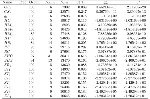
Table 1: Numerical results of SSA algorithm equipped with the repetition procedure.
Name Freq. Occur. NASA NF E CPU g∗m g∗
CS1 100 6 7302 0.039 3.55211e−11 2.11205e-20
CS2 99 12 28573 0.247 9.36766e−11 3.89995e-13
g1 100 6 12696 0.078 −1.0e+02 -1.0e+02
HC 100 5 19017 0.116 -1.03163e+00 -1.03163e+00
HM1 100 5 8823 0.036 3.10239e-08 1.95652e-15
HM2 100 5 10426 0.042 -4.81447e+00 -4.81447e+00
HM3 85 5 27448 0.128 7.88236e-09 2.98634e-12
HP 100 5 24636 0.195 4.79688e-08 4.65555e-08
HS1 84 14 16811 0.205 -1.76542e+02 -1.76542e+02
P S 98 15 29716 0.297 3.05417e-011 3.16409e-12
RC 90 6 27693 0.175 3.97887e-01 3.97887e-01
SHC 97 31 36311 0.616 -1.86731e+02 -1.86731e+02
SHS 91 13 13470 0.164 -2.40625e+01 -2.40625e+01
SR1 100 5 13630 0.088 4.73862e-10 4.11784e-12
ST1 100 5 14932 0.086 -4.07462e-01 -4.07462e-01
ST2 100 5 27470 0.152 -1.80587e+01 -1.80587e+01
ST3 100 5 18374 0.108 -2.27766e+02 -2.27766e+02
ST4 100 5 28201 0.155 -2.42941e+03 -2.42941e+03
ST5 100 9 25304 0.156 -2.47765e+04 -2.47765e+04
ST6 100 9 30016 0.184 -2.49293e+05 -2.49293e+05
Table 2: Numerical results of SSA algorithm equipped with the projection procedure.
Name Freq. Occur. NASA NF E CPU g∗m g∗
CS1 100 6 12502 0.059 1.78308e-10 4.67848e-15
CS2 98 13 39034 0.336 5.58567e-11 8.56119e-13
g1 85 4 3449 0.027 -1.0e+02 -1.0e+02
HC 100 5 17212 0.105 -1.03163e+00 -1.03163e+00
HM1 100 5 6338 0.03 2.19735e-09 4.20732e-15
HM2 100 5 7928 0.037 -4.81447e+00 -4.81447e+00
HM3 100 5 25842 0.12 3.28845e-09 1.07687e-11
HP 100 5 21308 0.164 4.71572e-08 4.65129e-08
HS1 72 12 13571 0.169 -1.76542e+02 -1.76542e+02
P S 96 16 42373 0.412 1.90246e-11 2.50598e-14
RC 100 7 25294 0.138 3.97887e-01 3.97887e-01
SHC 94 28 29183 0.494 -1.86731e+02 -1.86731e+02
SHS 91 13 14554 0.183 -2.40625e+01 -2.40625e+01
SR1 100 5 17707 0.127 6.79291e-10 5.04302e-12
ST1 100 5 33652 0.202 -4.07462e-01 -4.07462e-01
ST2 100 5 15490 0.084 -1.80587e+01 -1.80587e+01
ST3 100 5 26065 0.138 -2.27766e+02 -2.27766e+02
ST4 100 5 23282 0.12 -2.42941e+03 -2.42941e+03
ST5 100 8 34704 0.237 -2.47765e+04 -2.47765e+04
ST6 100 7 32551 0.184 -2.49293e+05 -2.49293e+05
ZL2 100 6 8439 0.048 -1.20312e+01 -1.20312e+01
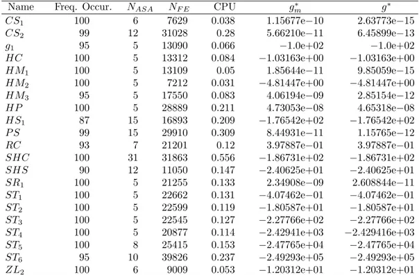
Table 3: Numerical results of SSA algorithm equipped with the reflection technique.
Name Freq. Occur. NASA NF E CPU g∗m g∗
CS1 100 6 7629 0.038 1.15677e−10 2.63773e−15
CS2 99 12 31028 0.28 5.66210e−11 6.45899e−13
g1 95 5 13090 0.066 −1.0e+02 −1.0e+02
HC 100 5 13312 0.084 −1.03163e+00 −1.03163e+00
HM1 100 5 13109 0.05 1.85644e−11 9.85059e−15
HM2 100 5 7212 0.031 −4.81447e+00 −4.81447e+00
HM3 95 5 17550 0.083 4.06194e−09 2.85154e−12
HP 100 5 28889 0.211 4.73053e−08 4.65318e−08
HS1 87 15 16893 0.209 −1.76542e+02 −1.76542e+02
P S 99 15 29910 0.309 8.44931e−11 1.15765e−12
RC 93 7 21201 0.12 3.97887e−01 3.97887e−01
SHC 100 31 31863 0.556 −1.86731e+02 −1.86731e+02
SHS 90 12 11050 0.147 −2.40625e+01 −2.40625e+01
SR1 100 5 21255 0.133 2.34908e−09 2.608844e−11
ST1 100 5 22662 0.131 −4.07462e−01 −4.07462e−01
ST2 100 5 22599 0.119 −1.80587e+01 −1.80587e+01
ST3 100 5 22545 0.127 −2.27766e+02 −2.27766e+02
ST4 100 5 20877 0.114 −2.42941e+03 −2.429416e+03
ST5 100 8 25415 0.153 −2.47765e+04 −2.47765e+04
ST6 95 10 39826 0.237 −2.49293e+05 −2.49293e+05
ZL2 100 6 9009 0.053 −1.20312e+01 −1.20312e+01
In one dimensional problems, all variants of the SSA algorithm find all global solutions requiring a small number of function evaluations. The three variants find good precision approximations to the global solutions, with absolute errors (difference between the average best function value and the best function value obtained in all runs) smaller than 10−7. For the other tested problems we obtain absolute
errors smaller than 10−6 or relative errors smaller than 10−6.
The three variants of the SSA algorithm have a similar behavior. Table 4 reports the cumulative results of each variant for the 21 tested problems. The column Freq. Occur. displays the mean values of the previous tables.
Table 4: Cumulative results of the SSA variants.
Variant Freq. Occur. NASA NF E CPU
SSA with repetition 97.33% 177 431494 3.333 SSA with projection 96.95% 170 450478 3.414 SSA with reflection 97.76% 177 426924 3.251
It seems that the SSA algorithm equipped with the reflection procedure need less number of function evaluations, CPU time and has a higher mean frequency of occurrence considering that the number of ASA calls is the same as in the repetition procedure.
In some well-known multimodal problems, the existence of many local maximizers makes it quite difficult for most global algorithms to determine the global solution. The algorithms usually stop pre-maturely in a local solution. We decided to analyze the behavior of our SSA algorithm with the reflection procedure in this class of problems. Therefore, Table 5 reports on the obtained numerical results with problems that have only one global but many local solutions.
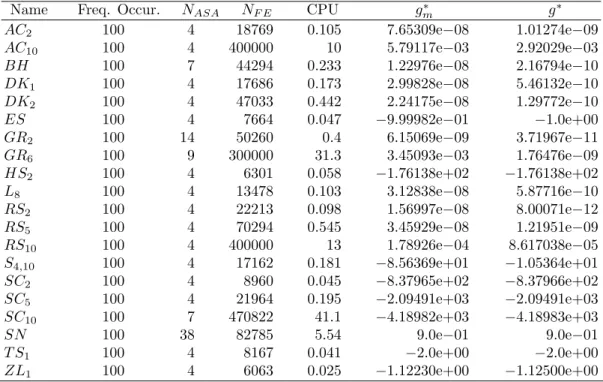
Table 5: Numerical results of test problems with one global and more than ten local solutions.
Name Freq. Occur. NASA NF E CPU g∗m g∗
AC2 100 4 18769 0.105 7.65309e−08 1.01274e−09
AC10 100 4 400000 10 5.79117e−03 2.92029e−03
BH 100 7 44294 0.233 1.22976e−08 2.16794e−10
DK1 100 4 17686 0.173 2.99828e−08 5.46132e−10
DK2 100 4 47033 0.442 2.24175e−08 1.29772e−10
ES 100 4 7664 0.047 −9.99982e−01 −1.0e+00
GR2 100 14 50260 0.4 6.15069e−09 3.71967e−11
GR6 100 9 300000 31.3 3.45093e−03 1.76476e−09
HS2 100 4 6301 0.058 −1.76138e+02 −1.76138e+02
L8 100 4 13478 0.103 3.12838e−08 5.87716e−10
RS2 100 4 22213 0.098 1.56997e−08 8.00071e−12
RS5 100 4 70294 0.545 3.45929e−08 1.21951e−09
RS10 100 4 400000 13 1.78926e−04 8.617038e−05
S4,10 100 4 17162 0.181 −8.56369e+01 −1.05364e+01
SC2 100 4 8960 0.045 −8.37965e+02 −8.37966e+02
SC5 100 4 21964 0.195 −2.09491e+03 −2.09491e+03
SC10 100 7 470822 41.1 −4.18982e+03 −4.18983e+03
SN 100 38 82785 5.54 9.0e−01 9.0e−01
T S1 100 4 8167 0.041 −2.0e+00 −2.0e+00
ZL1 100 4 6063 0.025 −1.12230e+00 −1.12500e+00
With the problems BH,SN,GR2 and GR6, the SSA algorithm was also able to detect some local
For the high dimensional problemsAC10,RS10,SC10, the SSA algorithm identifies the region where
the global maximum is located, but with a lower accuracy.
The function stretching efficiency is more evident in the problems GR2, GR6 and SN. We run
separately the ASA algorithm and obtained percentages of frequency of occurrence of 20%, 30% and 30%, respectively. When we use the SSA algorithm these percentages climb to 100% (see Table 5).
5.2
Comparison with other solvers
It does not seem an easy task to compare the performance of our algorithm with other multi-global solvers as some authors failed to report on important data, namely the number of function evaluations required to reach the solutions with a certain accuracy. For example, for the problemP S that was also solved by a version of PSO algorithm in [20], the authors claim to find all global solutions after 12 cycles of the method with accuracy 10−5, probably in a single run. No other information is reported concerning
this problem. In all 10 runs, our SSA algorithm found all solutions with accuracy 10−10 requiring on
average 15 ASA calls and 29910 function evaluations.
Meng et al. [17] proposed the adaptive swarm algorithm for multi-global optimization problems
and presented numerical results for the three problems: CS1, CS2 and HS1. Table 6 contains a brief
comparison. For the test functionHS1, Menget al. consider the feasible region [−5,5]2and only indicate
that the four global solutions were obtained after 17127 function evaluations. The SSA algorithm required 13002 function evaluations and 0.13 seconds of CPU time to reach the same solutions. For these cases, our SSA framework seems to perform favorably against the adaptive swarm algorithm.
Table 6: A comparison of results with those obtained by Menget al..
Adaptive swarm algorithm Stretched simulated annealing Freq. occur. Best solution Worst solution Freq. occur. Best solution Worst solution
CS1 93% 6.34×10⁻⁷ 1.05×10⁻³ 100% 4.43×10⁻¹³ 4.42×10⁻⁷
CS2 78% 5.12×10⁻⁵ 3.58×10⁻² 100% 3.09×10⁻¹⁰ 1.03×10⁻⁵
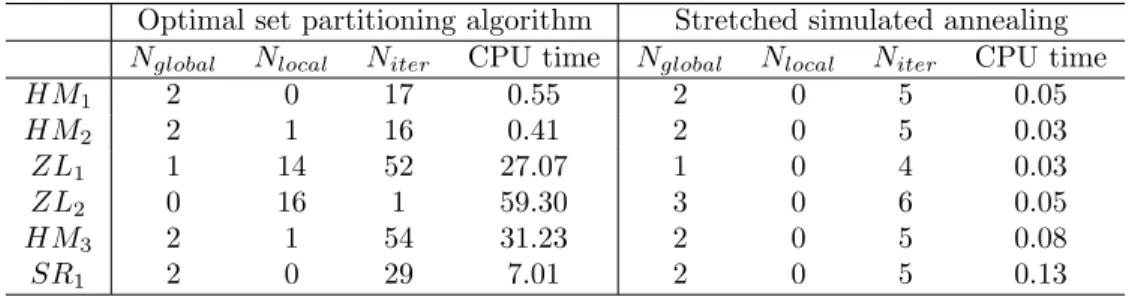
Kiseleva and Stepanchuk [14] proposed a global solver based on a method of optimal set partitioning to find all solutions of the problem (1). Some of their numerical results are presented in Table 7. The Kiseleva and Stepanchuk algorithm did not find the global solutions of problemZL2. The SSA algorithm
found all global solutions within a few number of iterations and a reduced CPU time. Considering these problems, our algorithm outperforms the one presented in [14].
Table 7: A comparison of results with those obtained by Kiseleva and Stepanchuk.
Optimal set partitioning algorithm Stretched simulated annealing
Nglobal Nlocal Niter CPU time Nglobal Nlocal Niter CPU time
HM1 2 0 17 0.55 2 0 5 0.05
HM2 2 1 16 0.41 2 0 5 0.03
ZL1 1 14 52 27.07 1 0 4 0.03
ZL2 0 16 1 59.30 3 0 6 0.05
HM3 2 1 54 31.23 2 0 5 0.08
SR1 2 0 29 7.01 2 0 5 0.13
6
Conclusions
In this work, we propose a new stochastic algorithm for locating all global solutions of multimodal optimization problems through the use of local applications of the function stretching technique and a variant of the adaptive simulated annealing method. Our computational experiments show that the SSA algorithm is capable of detecting with high rates of success all the global optima within an acceptable number of function evaluations. The numerical results also indicate that the SSA algorithm is a useful tool for detecting a global optimum when the problem has a large number of local solutions.
In our view, we may adapt the SSA algorithm to find all the global solutions as well as some local (non-global) ones, probably the ”best”, in the sense that these local solutions have function values that satisfy
|g(t∗)−g(t∗i)|< η
wheret∗ represents the global maximizer andt∗
i are the desired non-global maximizers, for a fixed
posi-tiveη. This issue is now under investigation.
References
[1] I. Bohachevsky, M. Johnson, and M. Stein,Generalized simulated annealing for function optimiza-tion, Technometrics28 (1986), no. 3, 209–217.
[2] R. Chelouah and P. Siarry, A continuous genetic algorithm designed for the global optimization of multimodal functions, Journal of Heuristics6(2000), 191–213.
[3] A. Corana, M. Marchesi, C. Martini, and S. Ridella,Minimizing multimodal functions of continuous
variables with the ”simulated annealing” algorithm, ACM Transactions on Mathematical Software
13(1987), no. 3, 262–280.
[4] A. Dekkers and E. Aarts,Global optimization and simulated annealing, Mathematical Programming
50(1991), 367–393.
[5] R. Desai and R. Patil, SALO: Combining simulated annealing and local optimization for efficient
global optimization, Proceedings of the 9th Florida AI Research Symposium (FLAIRS - 96), 1996,
pp. 233–237.
[6] I. Dixon and G. Szeg¨o,Towards global optimisation 2, North-Holland Publishing Company, 1978.
[7] P. Eriksson and J. Arora,A comparison of global optimization algorithms applied to a ride comfort optimization problem, Structural and Multidisciplinary Optimization24(2002), 157–167.
[8] C. Floudas,Recent advances in global optimization for process synthesis, design and control:
enclo-sure of all solutions, Computers and Chemical Engineering (1999), S963–973.
[9] R. Fourer, D. Gay, and B. Kernighan, A modeling language for mathematical programming, Man-agement Science36 (1990), no. 5, 519–554, http://www.ampl.com.
[10] A.-R. Hedar and M. Fukushima,Heuristic pattern search and its hybridization with simulated
an-nealing for nonlinear global optimization, Optimization Methods and Software19 (2004), no. 3-4,
291–308.
[11] L. Ingber,Adaptive simulated annealing (ASA): Lessons learned, Control and Cybernetics25(1996), no. 1, 33–54.
[13] D. Johnson, C. Aragon, L. McGeoch, and C. Schevon, Optimization by simulated annealing: An
experimental evaluation; part II, graph coloring and number partitioning, Operations Research 39
(1991), no. 3, 378–406.
[14] E. Kiseleva and T. Stepanchuk,On the efficiency of a global non-differentiable optimization
algo-rithm based on the method of optimal set partitioning, Journal of Global Optimization 25(2003),
209–235.
[15] P. Van Laarhoven and E. Aarts, Simulated annealing: Theory and applications, Mathematics and Its Applications, Kluwer Academic Publishers, 1987.
[16] K. Madsen,Test problems for global optimization, http://www2.imm.dtu.dk/∼km/GlobOpt/testex
2000.
[17] T. Meng, T. Ray, and P. Dhar, Supplementary material on parameter estimation using swarm algorithm, Preprint submitted to Elsevier Science (2004).
[18] X. Niu, An integrated system of optical metrology for deep sub-micron lithography, Ph.D. thesis, University of California, 1999.
[19] K. Parsopoulos, V. Plagianakos, G. Magoulas, and M. Vrahatis, Objective function stretching to alleviate convergence to local minima, Nonlinear Analysis47(2001), 3419–3424.
[20] K. Parsopoulos and M. Vrahatis, Modification of the particle swarm optimizer for locating all
the global minima, Artificial Neural Networks and Genetic Algorithms (V. Kurkova, N. Steele,
R. Neruda, and M. Karny, eds.), Springer, 2001, pp. 324–327.
[21] , Recent approaches to global optimization problems through particle swarm optimization,
Natural Computing1(2002), 235–306.
[22] H. Pohlheim, Gea - toolbox examples of objective functions, http://www.systemtechnik.tu-ilmenau.de/∼pohlheim/ga toolbox, 1997.
[23] C. Price,Non-linear semi-infinite programming, Ph.D. thesis, University of Canterbury, 1992.
[24] H. Romeijn and R. Smith,Simulated annealing for constrained global optimization, Journal of Global Optimization5(1994), 101–126.
[25] H. Romeijn, Z. Zabinsky, D. Graesser, and S. Neogi,New reflection generator for simulated annealing
in mixed-integer/continuous global optimization, Journal of Optimization Theory and Applications
101(1999), no. 2, 403–427.
[26] S. Salhi and N. Queen,A hybrid algorithm for identifying global and local minima when optimizing
functions with many minima, European Journal of Optimization Research155(2004), 51–67.
[27] R. Storn and K. Price,Differential evolution - a simple and efficient heuristic for global optimization over continuous spaces, Journal of Global Optimization11(1997), 341–359.
[28] H. Szu and R. Hartley,Fast simulated annealing, Physics Letters A122(1987), no. 3-4, 157–162.
[29] S.Sanmat´ıas T. Le´on and H. Vercher, A multi-local optimization algorithm, Top 6 (1998), no. 1, 1–18.
[30] C. Tsallis and D. Stariolo,Generalized simulated annealing, Physics Letters A233(1996).
[31] I. Tsoulos and I. Lagaris, Gradient-controlled, typical-distance clustering for global optimization, www.optimization.org (2004).
[33] Q. Zhang, J. Sun, E. Tsang, and J. Ford, Hybrid estimation of distribution algorithm for global
optimization, Engineering Computations21 (2004), no. 1.
Appendix
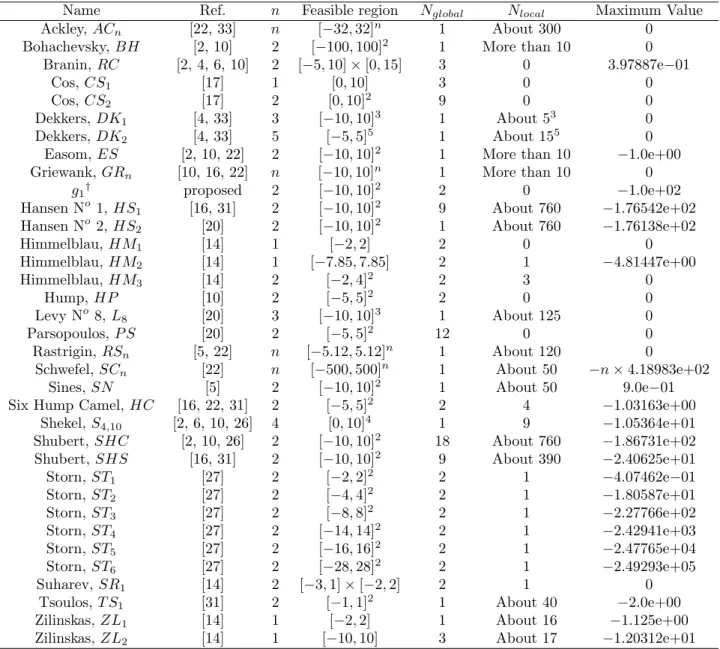
Table 8 shows the main characteristics of the multimodal test problems, namely the name of the problem, the reference from where we took the problem (Ref.), the number of variables (n), the feasible region, the number of known global maximizers (Nglobal), the number of known local (non-global) maximizers
(Nlocal) and the known global maximum value.
Table 8: Test problems.
Name Ref. n Feasible region Nglobal Nlocal Maximum Value
Ackley,ACn [22, 33] n [−32,32]n 1 About 300 0
Bohachevsky, BH [2, 10] 2 [−100,100]2 1 More than 10 0
Branin,RC [2, 4, 6, 10] 2 [−5,10]×[0,15] 3 0 3.97887e−01
Cos,CS1 [17] 1 [0,10] 3 0 0
Cos,CS2 [17] 2 [0,10]2 9 0 0
Dekkers,DK1 [4, 33] 3 [−10,10]3 1 About 53 0
Dekkers,DK2 [4, 33] 5 [−5,5]5 1 About 155 0
Easom,ES [2, 10, 22] 2 [−10,10]2 1 More than 10 −1.0e+00
Griewank,GRn [10, 16, 22] n [−10,10]n 1 More than 10 0
g1† proposed 2 [−10,10]2 2 0 −1.0e+02
Hansen No 1,HS1 [16, 31] 2 [−10,10]2 9 About 760 −1.76542e+02
Hansen No 2,HS2 [20] 2 [−10,10]2 1 About 760 −1.76138e+02
Himmelblau,HM1 [14] 1 [−2,2] 2 0 0
Himmelblau,HM2 [14] 1 [−7.85,7.85] 2 1 −4.81447e+00
Himmelblau,HM3 [14] 2 [−2,4]2 2 3 0
Hump,HP [10] 2 [−5,5]2 2 0 0
Levy No8,L
8 [20] 3 [−10,10]3 1 About 125 0
Parsopoulos,P S [20] 2 [−5,5]2 12 0 0
Rastrigin, RSn [5, 22] n [−5.12,5.12]n 1 About 120 0
Schwefel,SCn [22] n [−500,500]n 1 About 50 −n×4.18983e+02
Sines, SN [5] 2 [−10,10]2 1 About 50 9.0e−01
Six Hump Camel,HC [16, 22, 31] 2 [−5,5]2 2 4 −1.03163e+00
Shekel,S4,10 [2, 6, 10, 26] 4 [0,10]4 1 9 −1.05364e+01
Shubert,SHC [2, 10, 26] 2 [−10,10]2 18 About 760 −1.86731e+02
Shubert,SHS [16, 31] 2 [−10,10]2 9 About 390 −2.40625e+01
Storn,ST1 [27] 2 [−2,2]2 2 1 −4.07462e−01
Storn,ST2 [27] 2 [−4,4]2 2 1 −1.80587e+01
Storn,ST3 [27] 2 [−8,8]2 2 1 −2.27766e+02
Storn,ST4 [27] 2 [−14,14]2 2 1 −2.42941e+03
Storn,ST5 [27] 2 [−16,16]2 2 1 −2.47765e+04
Storn,ST6 [27] 2 [−28,28]2 2 1 −2.49293e+05
Suharev,SR1 [14] 2 [−3,1]×[−2,2] 2 1 0
Tsoulos,T S1 [31] 2 [−1,1]2 1 About 40 −2.0e+00
Zilinskas,ZL1 [14] 1 [−2,2] 1 About 16 −1.125e+00
Zilinskas,ZL2 [14] 1 [−10,10] 3 About 17 −1.20312e+01
†g