Problems with Parallel Stretched Simulated
Annealing
Ana I. Pereira1,2(B)and Jos´e Rufino1,3
1
Polytechnic Institute of Bragan¸ca, 5301-857 Bragan¸ca, Portugal
{apereira,rufino}@ipb.pt
2
Algoritmi R&D Centre, University of Minho, Campus de Gualtar, 4710-057 Braga, Portugal
3
Laboratory of Instrumentation and Experimental Particle Physics, University of Minho, Campus de Gualtar, 4710-057 Braga, Portugal
Abstract. Constrained multilocal programming optimization problems may be solved by solving a sequence of unconstrained problems. In turn, those unconstrained problems may be solved using techniques like the Stretched Simulated Annealing (SSA) method. In order to increase the solving performance and make possible the discovery of new optima, parallel approaches to SSA have been devised, like Parallel Stretched Simulated Annealing (PSSA). Recently, Constrained PSSA (coPSSA) was also proposed, coupling the penalty method with PSSA, in order to solve constrained problems. In this work, coPSSA is explored to solve four test problems using thel1penalty function. The effect of the variation of the reduction factor parameter of thel1penalty function is also studied.
Keywords: Unconstrained optimization
·
Parallel computing1
Introduction
Multilocal programming aims to identify all local maximizers of unconstrained or constrained nonlinear optimization problems. More formally, a constrained multilocal programming problem may be defined by the following formulation:
maxf(x)
s.t.hk(x) = 0, k∈E gj(x)≤0, j∈I
−li≤xi≤li, i= 1, . . . , n
(1)
where at least one of then-dimensional functionsf, hk, gj :Rn→Ris nonlinear, and E andI are index sets of equality and inequality constraints, respectively. Since concavity is not assumed, the nonlinear optimization problem can have many global and local (non-global) maxima. Consider the feasible region (search space) defined by R ={x∈ Rn : −li ≤ xi ≤ li, i = 1, . . . , n; hk(x) = 0, k ∈
c
Springer International Publishing Switzerland 2015
E; gj(x)≤0, j∈I}. Thus, the purpose of the maximization problem (1) is to find all local maximizers,i.e., all pointsx∗∈ Rsuch that condition (2) holds:
∀x∈Vǫ(x∗)∩ R, f(x∗)≥f(x). (2) where Vǫ(x∗) is a neighborhood ofx∗, with a positive rayǫ.
It is also assumed that problem (1) has a finite number of isolated global and local maximizers. The existence of multi-solutions (local and global) makes this problem a great challenge that may be tackled with parallel solving techniques. Methods for solving multilocal optimization problems include evolutionary algorithms, such as genetic [1] and particle swarm [13] algorithms, and additional contributions, like [6,15,20,23,24]. Stretched Simulated Annealing (SSA) was also proposed [14], combining simulated annealing and a stretching function technique, to solve unconstrained multilocal programming problems.
In previous work [16,18], Parallel Stretched Simulated Annealing (PSSA) was introduced as a parallel version of SSA, based on the decomposition of the feasible region in several subregions to which SSA is independently applied by a set of processors. Several domain decomposition and distribution approaches were explored, leading to successively increasing levels of numerical efficiency.
More recently, the parallel solving of constrained multilocal programming problems was also proposed, through coPSSA [19] (constrained PSSA), that couples the penalty method with PSSA. Basically, coPSSA creates a homoge-neous partition of the iteration set of thel1 penalty function [11]; each iteration
subset is run in parallel, by different processors of a shared memory system, and each specific iteration invokes PSSA; this, in turn, involves additional processors; these processors are usually from a distributed memory cluster, but may also be from the same shared memory host, once PSSA is a MPI-based application [8]. In this paper, coPSSA is explored, with thel1penalty function, to solve four
well known test problems [4], in order to analyze the kind of performance gains that may be expected with a reasonable set of parallel configurations. Moreover, the effect of the variation of the reduction factor parameterτ of thel1 function
is analyzed to investigate the existence of values leading to faster convergence. The rest of the paper is organized as follows. Section2revises the basic ideas behind SSA and PSSA. Section 3 covers the basics of penalty method with l1
penalty function, and provides some details on coPSSA design and implementa-tion. Section 4 presents performance and numerical results from the evaluation of coPSSA. Finally, Section 5concludes and defines directions for future work.
2
Unconstrained Optimization
2.1 Stretched Simulated Annealing
Stretched Simulated Annealing (SSA) is a multilocal programming method that solves bound constrained optimization problems. These may be described as:
max
where ϕ:Rn →Ris a given n-dimensional multimodal objective function and X is the feasible region defined byX ={x∈Rn : −li ≤xi≤li, i= 1, ..., n}.
SSA solves a sequence of global optimization problems in order to compute the local solutions of the maximization problem (3). The objective function of each global problem is generated using a stretching function technique [12].
Letx∗ be a solution of problem (3). The mathematical formulation of the global optimization problem is as follows:
max
x∈XΦl(x)≡
ˆ
φ(x) ifx∈Vε(x∗)
ϕ(x) otherwise (4)
whereVε(x∗) is the neighborhood of solutionx∗ with a rayε >0. The ˆφ(x) function is defined as
ˆ
φ(x) = ¯φ(x)−δ2[sign(ϕ(x
∗)−ϕ(x)) + 1]
2 tanh(κ( ¯φ(x∗)−φ¯(x)) (5) whereδ1,δ2 andκare positive constants, and ¯φ(x) is
¯
φ(x) =ϕ(x)−δ1
2 x−x
∗ [sign(ϕ(x∗)−ϕ(x)) + 1]. (6)
To solve the global optimization problem (4) the Simulated Annealing (SA) method is used [5]. The Stretched Simulated Annealing algorithm stops when no new optimum is identified afterrconsecutive runs. [15,16] provide more details.
2.2 Parallel Stretched Simulated Annealing
As a parallel implementation of the SSA method, PSSA was thoroughly described in previous work [16]. In this section, only a brief description is pro-vided.
of the feasible region, leading to an unpredictable number of subregions, of vari-able size, dynamically generated and processed on-demand, until certain stop criteria are met. PSSA-HoS and PSSA-HoD have the same numerical efficiency (i.e., both find the same number of optima), but PSSA-HoD is faster due to its workload auto-balancing. PSSA-HeS usually finds more optima, but is also the slowest of the PSSA variants, once it typically searches many more subregions.
PSSA was written in C, runs on Linux systems, and it builds on MPI [8] (thus following the message passing paradigm). It is a SPMD (Single Program, Multiple Data) application that operates in amaster-slavesconfiguration (slave tasks run SSA in subregions, under coordination of amastertask), and may be deployed in shared-memory systems and/or in distributed-memory clusters.
3
Constrained Optimization
3.1 l1 Penalty Method
There are three main classes of methods to solve constrained optimization prob-lems [9,25]: 1) methods that use penalty functions, 2) methods based on biasing feasible over infeasible solutions, and 3) methods that rely on multi-objective optimization concepts. In this work constraints are handled using a class 1 method with the l1 penalty function. This function is a classic penalty [11]
defined by
ϕ(x, μ) =f(x)− 1
μ
⎡
⎣
k∈E
|hk(x)|+ j∈I
[gj(x)]+
⎤
⎦
where μ is a positive penalty parameter that progressively decreases to zero, alongkmaxiterations. A lower boundμminis defined andμis updated as follows:
μk+1= max
τ μk, μmin (7)
where k∈ {1, ..., kmax} represents the iteration,μmin≈0 and 0< τ <1.
To solve the constrained problem (1), the penalty method solves a sequence of bound constrained problems, based on the l1 penalty function, as defined by
max x∈Xϕ(x, μ
k
). (8)
Problem (8) is solvable using PSSA. It is possible to prove that the solutions sequence{x∗(μk)}from (8) converges to the solutionx∗ of problem (1) [11,15]. The penalty method stops when a maximum number of iterations (kmax) is reached, or successive solutions are similar, accordingly with the next criteria:
f(xk)−f(xk−1)
≤ǫ1 ∧
xk−xk−1
≤ǫ2 (9)
where kis a given iteration of the penalty method.
The optimum value for the reduction factorτ of the update expression (7) is an open research issue in the optimization field [10,21]. This paper presents an analysis of the effect of the variation ofτ in thel1 penalty function method,
3.2 Constrained PSSA
Constrained PSSA (coPSSA) was already introduced in [19], albeit in the context of a simpler evaluation scenario than the one explored in this paper. Here coPSSA is revised, and some clarification is provided on its design and implementation.
As stated in the previous section, problem (8) may be solved using SSA, including its parallel implementations, like PSSA. However, coupling PSSA with a serial implementation of the penalty method is of limited benefit performance-wise: in the end, some extra optima may be detected (due to the extra efforts of PSSA), but the penalty method will not run faster. A possible approach to increase the performance of the penalty method is to parallelize its execution.
As it happens, the parallelization of the penalty method is trivial: this method will execute a certain maximum number of times or iterations, as defined by the parameterkmax; each iteration uses successively lower values of the penalty parameterμ; these values are completely deterministic, as given by (7); therefore, a partition of the iteration space{1, ..., kmax}may be defined, a priori, such that mutually disjoint subintervals of this space are assigned to different processors or search tasks (with one task per processor); each task will then run the penalty method along its iteration subspace; as soon as a task reaches convergence (in accordance to criteria (9)), the others will stop the search (before moving on to its next iteration, a task checks if other has already converged to the solutions). Having different processors/tasks starting the optima search with different values of μ, scattered along the interval of possible values {μ1, ..., μkmax}, may allow to reach convergence sooner, as compared to a single full sequential scan of that interval. However, it was noted that this strategy does not necessarily pay off; it must be tested for each and different constrained optimization problem, once the value(s) ofμthat lead to convergence are unpredictable by nature.
coPSSA adopts the strategy above, for the parallelization of the penalty method, by performing a homogeneous decomposition of the iteration space: givenP search tasks andkmax iterations, any search tasktp (withp= 1, ..., P) will iterate through approximately the same number of iterations,w=⌈kmax
P )⌉, where ⌈x⌉ is the smallest integer value not less thanx; the iteration subinter-val for a task tp is then{kplef t, ..., k
p
right}, where k p
lef t = ((p−1)×w) + 1 and kpright = p×w; when a uniform width w is not possible (kmaxmod P = 0), coPSSA makes the necessary adjustments in the last iteration subinterval (the one for task p); for instance, with kmax = 100 and P = 2, it is obtained w = ⌈50.0⌉ = 50 and so t1 will iterate through {1, ...,50} and t2 will iterate
through{51, ...,100}; withP = 3 it is obtainedw=⌈33.3(3)⌉= 34, and sot1,t2
andt3 will iterate through{1, ...,34},{35, ...,68}and{69, ...,100}, respectively.
Like PSSA, coPSSA was also coded in C, for performance reasons, and also to reuse previous code from one of the authors. In coPSSA, search tasks are con-ventional UNIX processes, that synchronize and exchange data using classical System V IPC mechanisms, like semaphores and shared memory1. When coPSSA
1
starts, it forksPchild processes (one per search task), whereP is usually defined to be the number of CPU-cores of the host running coPSSA. Each child (search task) will then run the penalty method through a specific iteration subinterval; for each particular iteration, PSSA must be invoked; this is simply accomplished using thesystemprimitive, that spawns second-level childs to run thempiexec
command2; in turn, this command runs PSSA, in a MPI master-slaves
config-uration, in a set of hosts / CPU-cores that are defined by coPSSA; basically, coPSSA is supplied with a base MPI “machinefile”, from which extracts the computing resources to be assigned to each PSSA execution; the results pro-duced by PSSA executions are written in specific files, which are then checked by the search tasks, in order to detect a possible convergence.
Fig. 1.The coPSSA application and its interactions with PSSA (tpare coPSSA search tasks;mandsare PSSA tasks (master and slaves);fpare result files from PSSA)
Figure1is a representation of coPSSA, including its interactions with PSSA. coPSSA may thus be viewed as a hybrid application, in the sense that combines its internal usage of shared-memory based parallelism, with an external compo-nent (PSSA) specially suited to exploit distributed-memory parallelism.
4
Evaluation
4.1 Setup
The experimental evaluation performed in the context of this work was carried in a commodity cluster of 9 hosts (1 frontend, and 8 worker nodes), with one Intel Core-i7 4790K 4.0GHz quad-core CPU per node, under Linux ROCKS version 6.1.1, with the Gnu C Compiler (GCC) version 4.4.7 and OpenMPI version 1.5.4. coPSSA was always executed in the cluster frontend, with the number of search tasks (P) ranging from 1 to 8 (no overload was observed for P > 4,
2
despite the frontend having only a 4-core CPU). PSSA executions took place in the 8 worker nodes; these offer a total of 32 CPU-cores, fully specified in the base MPI hostfile supplied to coPSSA, that are used, four at a time, to service the PSSA execution requests of each coPSSA task; thus, each PSSA execution always consumed 4 cores, with 1 core for the master process, and 3 cores for slave processes; in order to fully utilize these 3 cores, the number of subregions for each PSSA execution was set to be as close as possible (in excess) of 3; for 2-dimensional problems, like the ones tested, this implies 4 subregions [16]. The PSSA variant used throughout the tests was always PSSA-HoD: not only it is appropriate for a fixed number of subregions, but is also the fastest variant.
All tests shared the penalty algorithm parameterskmax=100,μ0=1.0,μmin=
10−6 and τ ∈ {0.1, ...,0.9}, and the convergence parameters ǫ
1 = ǫ2 = 10−4.
The PSSA numerical parameters werer= 5,δ1= 1.5,δ2= 0.5 andκ= 0.05.
4.2 Search Times
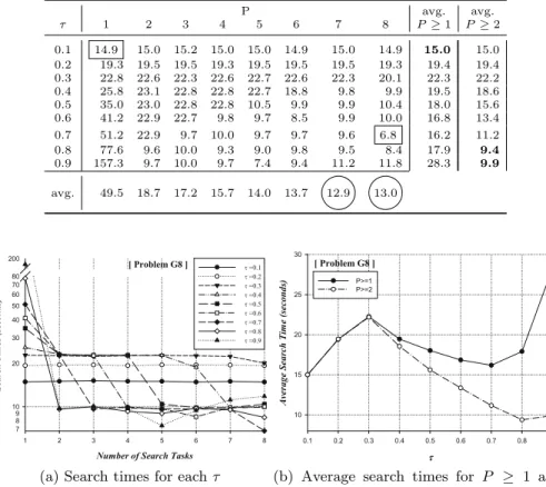
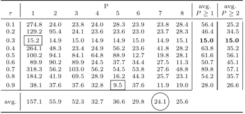
Tables4to7 show the search times measured for the selected benchmark prob-lems, for all valid combinations of P (number of coPSSA search tasks) and τ (the penalty reduction factor under evaluation), with P = 1,2, ...,8 and τ = 0.1,0.2, ...,0.9. The search times are the times required by coPSSA to converge to the constrained problem optima. Figures 2 to 5 represent the data of the tables, with four subfigures per table, that offer four different and complemen-tary perspectives on search times (the first two – (a) and (b) – build on a hori-zontal reading of the table, and the last two – (c) and (d) – build on a vertical reading):
(a) “Search times for eachτ”: one curve perτ value, based on the search times obtained with a fixedτ, when varying the number P of search tasks; allows to verify the influence of the variation of the degree of search parallelism (P) on the search times produced by a specificτ; allows also to identify the τ value that ensures the lowest (absolute minimum) search times;
(b) “Average search times for P ≥1 and P ≥2”: one curve, where each point is the average of the search times obtained with a fixedτ and all possible values of P (i.e., P ≥ 1); another curve, where each point is the average of the search times obtained with a fixed τ and all values of P ≥ 2; the first curve allows to deduce the bestτ, irregardless of the use of sequential (P = 1) or parallel (P ≥2) searches; the second curve allows to conclude whichτ value is the best when only parallel searches are made;
(c) “Search times for eachP”: one curve perP value, based on the search times obtained with a fixedP, when varyingτ; allows to verify the influence of the variation of the value ofτ on the search times produced by a specificP; allows also to identify theP value that ensures the lowest search times; (d) “Average search times for all τ values”: a single curve, where each point
For each of the above perspectives, these are the main conclusions that may be derived from the experimental data3:
(a) in all problems, when increasing the number of search tasks, the trend fol-lowed by the search times for each τ is mostly downwards, eventually fol-lowed by stabilization; this trend is more regular for Problems G6 and G8 (see Figures 2a and 3a), slightly less regular in Problem G12 (see Figure 5a), and much more irregular in Problem G11 (see Figure 4a); it is also possible to identify the values ofτ that attain the absolute minimum search times; these times are boxed (within a tolerance of 5%), in Tables4to7; the corresponding values ofτ are gathered in the following table:
Table 1.Values ofτ that ensure the absolute minimum search times
Problem P= 1 P≥2
G6 0.1 0.5 , 0.6
G8 0.1 0.7
G11 0.3 0.9
G12 0.1 0.6 to 0.9
the previous table allows to conclude that when only sequential searches are used (P = 1), the absolute minimum values for search times are attained with small values ofτ; however, if only parallel searches are conducted (P ≥2), the lowest search times are achieved with higher (mid range to maximum) values of τ; one should note, though, that these observations cannot be generalized, because theτvalues that produce the absolute minimum search times may not be the ones that produces the lowest average search times; (b) the values of τ that ensure the lowest average search times depend on the
specific problem, and also depend on whether both sequential or parallel searches are admitted (P ≥1), or only parallel searches (P≥2) are allowed; in Tables 4 to 7, the columns “avg.P ≥ 1” and “avg. P ≥ 2” show the average search times attained by eachτ, whenP ≥1 andP ≥2, respectively; in each column, the lowest average search time is in bold (within a tolerance of 5%); the related values ofτ are gathered in the following table:
Table 2.Values ofτ that ensure the lowest average search times
Problem P≥1 P≥2
G6 0.1 0.1 to 0.6
G8 0.1 0.8 , 0.9
G11 0.3 0.3
G12 0.1 0.1 to 0.6
the previous table allows to conclude that if using a sequential or a parallel search is indifferent (P ≥1), then single small values ofτ are best in order 3
Note: for Problem G6, no values are shown forτ = 0.9, because no convergence was reached within the maximum ofk
to attain the lowest search times, on average (coincidentally, such values ofτ match the values in Table1that ensure the absolute minimum search times forP = 1); however, if only parallel searches are admissible (P ≥2), there may be several best values ofτ to chose from, like in problems G6 and G12, that share the same range of values (0.1 to 0.6), or like in problem G8, with another range (0.8 to 0.9); problem G11, though, is an exception, because the bestτvalue is always the same (0.3) for sequential and parallel searches; (c) when increasing τ, problem G6 (Figure 2c) and problem G12 (Figure 5c) exhibit a similar trend on the search times for eachP (these times progres-sively increase for P = 1, but for P ≥ 2 they are substantially lower and stable, and only start to increase for higher values of τ); for problem G8 (Figure 3c), the trend is also upwards for P = 1, but now is reversal for P≥2 (asτ values increase, the search times will decay); finally, for problem G11 (Figure4c), the pattern is very irregular, independently ofP(increasing τ may lead to an unpredictable surge or decline of search times);
(d) irregardless ofτ, the use of parallel searches typically pays off for all problems (in general, increasing the level of parallelism (P) will decrease the search times); this downwards trend is more regular in problems G8 (Figure3d), G11 (Figure4d), and G12 (Figure5d), where the lowest average search times are achieved with the higher values ofP (values 7 and/or 8); in problem G6 (Figure2d), bothP = 4 andP = 7 provide the best average search times; all these times are shown encircled in the tables (within a tolerance of 5%).
4.3 Number of Optima
Another important issue is the number of optima found. Table 3 shows that number as an average: for each problem, sequential only (P = 1) and parallel only (P ≥2) searches are considered; for each of these categories, it is presented the mean of the number of optima found with all values ofτ tested (0.1,...,0.9); along with the mean, the coefficient of variation is also presented, in parenthesis.
Table 3.Average number of optima found (and coefficient of variation)
Problem P= 1 P≥2
G6 4.9 (20.3%) 5.7 (12.7%)
G8 6.0 (0%) 6.0 (0%)
G11 11.4 (21.5%) 11.9 (18.4%) G12 10.8 (7.7%) 10.2 (6.9%)
Table 4.Search times values for Problem G6 (seconds)
P avg. avg.
τ 1 2 3 4 5 6 7 8 P≥1 P≥2
0.1 33.7 7.7 7.7 7.7 7.7 7.7 7.7 7.7 10.9 7.7
0.2 41.8 7.7 7.7 7.7 7.7 7.7 7.7 7.7 11.9 7.7
0.3 70.7 7.7 7.7 7.7 7.7 7.7 7.7 7.7 15.6 7.7
0.4 95.8 7.7 7.7 7.7 7.7 7.7 7.7 7.6 18.7 7.7
0.5 85.8 7.7 7.7 7.7 7.7 7.7 7.1 7.8 17.4 7.6
0.6 142.4 7.7 7.7 7.7 7.9 8.2 7.2 8.7 24.7 7.8
0.7 159.9 7.8 7.7 7.8 9.0 7.6 8.8 8.7 27.1 8.2
0.8 263.2 91.3 31.7 8.7 14.8 17.6 8.7 12.7 56.10 26.5 0.9
avg. 111.7 18.1 10.7 7.8 8.8 9.0 7.8 8.6
(a) Search times for eachτ (b) Average search times for P ≥ 1 and P ≥ 2
(c) Search times for eachP (d) Average search times for allτ values
Table 5.Search times values for Problem G8 (seconds)
P avg. avg.
τ 1 2 3 4 5 6 7 8 P≥1 P≥2
0.1 14.9 15.0 15.2 15.0 15.0 14.9 15.0 14.9 15.0 15.0 0.2 19.3 19.5 19.5 19.3 19.5 19.5 19.5 19.3 19.4 19.4 0.3 22.8 22.6 22.3 22.6 22.7 22.6 22.3 20.1 22.3 22.2 0.4 25.8 23.1 22.8 22.8 22.7 18.8 9.8 9.9 19.5 18.6 0.5 35.0 23.0 22.8 22.8 10.5 9.9 9.9 10.4 18.0 15.6 0.6 41.2 22.9 22.7 9.8 9.7 8.5 9.9 10.0 16.8 13.4
0.7 51.2 22.9 9.7 10.0 9.7 9.7 9.6 6.8 16.2 11.2
0.8 77.6 9.6 10.0 9.3 9.0 9.8 9.5 8.4 17.9 9.4
0.9 157.3 9.7 10.0 9.7 7.4 9.4 11.2 11.8 28.3 9.9
avg. 49.5 18.7 17.2 15.7 14.0 13.7 12.9 13.0
(a) Search times for eachτ (b) Average search times for P ≥ 1 and P ≥ 2
(c) Search times for eachP (d) Average search times for allτ values
Table 6.Search times values for Problem G11 (seconds)
P avg. avg.
τ 1 2 3 4 5 6 7 8 P≥1 P≥2
0.1 274.8 24.0 23.8 24.0 28.3 23.9 23.8 28.4 56.4 25.2 0.2 129.2 95.4 24.1 23.6 23.6 23.0 23.7 28.3 46.4 34.5 0.3 15.2 14.9 15.0 14.9 14.9 15.0 14.9 15.1 15.0 15.0
0.4 264.1 48.3 23.4 24.9 56.2 23.6 41.8 28.2 63.8 35.2 0.5 100.2 94.1 84.1 64.8 88.9 12.7 19.8 28.1 61.6 56.1 0.6 89.9 90.2 89.9 24.5 37.7 34.4 27.5 11.3 50.7 45.1 0.7 318.3 56.2 103.0 56.2 54.5 53.8 27.6 48.8 89.8 57.1 0.8 184.2 41.9 69.5 28.9 16.2 44.3 25.7 23.1 54.2 35.7 0.9 38.1 37.6 37.6 32.8 9.5 37.6 11.9 19.0 28.0 26.6 avg. 157.1 55.9 52.3 32.7 36.6 29.8 24.1 25.6
(a) Search times for eachτ. (b) Average search times for P ≥ 1 and P ≥ 2
(c) Search times for eachP (d) Average search times for allτ values
Table 7.Search times values for Problem G12 (seconds)
P avg. avg.
τ 1 2 3 4 5 6 7 8 P≥1 P≥2
0.1 67.6 14.1 14.1 14.1 14.1 14.1 14.1 14.1 20.8 14.1
0.2 79.5 14.1 14.1 14.1 14.1 14.1 14.1 14.1 22.3 14.1
0.3 87.3 14.1 14.1 14.1 14.1 14.1 14.1 13.5 23.2 14.0
0.4 116.9 14.2 14.1 14.1 14.1 13.5 14.1 14.1 26.9 14.0
0.5 154.9 14.1 14.1 14.1 14.1 14.3 14.1 15.2 31.8 14.3
0.6 142.4 14.1 14.1 14.1 14.1 16.3 13.1 16.4 30.6 14.6
0.7 202.1 21.4 14.2 15.2 16.3 16.3 13.3 13.1 39.0 15.7 0.8 92.4 90.1 13.1 36.7 16.3 15.1 16.3 15.0 36.9 29.0 0.9 124.7 125.6 83.6 19.1 45.1 12.9 13.3 12.8 54.6 44.6 avg. 118.7 35.8 21.7 17.3 18.0 14.5 14.1 14.3
(a) Search times for eachτ (b) Average search times for P ≥ 1 and P ≥ 2
(c) Search times for eachP (d) Average search times for allτ values
5
Conclusions and Future Work
In this paper coPSSA is explored, as a hybrid application that solves constrained optimization problems, by integrating a numerical l1 penalty method with a
parallel solver of unconstrained (bound constrained) problems (PSSA).
The effect of the variation of the number of search tasks, and of the penalty parameter reduction factor (τ) was studied, in the context of the l1 penalty
function. With base on the analysis of the results obtained with the four tested problems, it is possible to conclude: i) increasing the number of search tasks typically decreases the search times; ii) for the tested problems, smaller values of τ typically imply lower average search times; iii) for some problems, the number of optima found does not depend on the number of search tasks neither on the value ofτ, while other problems are sensitive to the variation of those factors.
In the future, the research team intends to refine this work, by solving more constrained problems (including problems with more than 2 dimensions), and exploring higher levels of parallelism (i.e., by running coPSSA withP >>8). Acknowledgments. This work was been supported by FCT (Funda¸c˜ao para a Ciˆencia e Tecnologia) in the scope of the project UID/CEC/00319/2013.
References
1. Chelouah, R., Siarry, P.: A continuous genetic algorithm designed for the global optimization of multimodal functions. Journal of Heuristics6, 191–213 (2000) 2. Eriksson, P., Arora, J.: A comparison of global optimization algorithms applied
to a ride comfort optimization problem. Structural and Multidisciplinary Opti-mization24, 157–167 (2002)
3. Floudas, C.: Recent advances in global optimization for process synthesis, design and control: enclosure of all solutions. Computers and Chemical Engineering, 963–973 (1999)
4. Hedar, A.-R.: Global Optimization Test Problems. http://www-optima.amp.i. kyoto-u.ac.jp/member/student/hedar/Hedar files/TestGO.htm
5. Ingber, L.: Very fast simulated re-annealing. Mathematical and Computer Mod-elling12, 967–973 (1989)
6. Kiseleva, E., Stepanchuk, T.: On the efficiency of a global non-differentiable opti-mization algorithm based on the method of optimal set partitioning. Journal of Global Optimization 25, 209–235 (2003)
7. Le´on, T., Sanmat´ıas, S., Vercher, H.: A multi-local optimization algorithm. Top 6(1), 1–18 (1998)
8. Message Passing Interface Forum.http://www.mpi-forum.org/
9. Michalewicz, Z.: A survey of constraint handling techniques in evolutionary com-putation methods. In: Proceedings of the 4th Annual Conference on Evolutionary Programming, pp. 135–155 (1995)
10. Mongeau, M., Sartenaer, A.: Automatic decrease of the penalty parameter in exact penalty function methods. European Journal of Operational Research83, 686–699 (1995)
12. Parsopoulos, K., Plagianakos, V., Magoulas, G., Vrahatis, M.: Objective function stretching to alleviate convergence to local minima. Nonlinear Analysis47, 3419– 3424 (2001)
13. Parsopoulos, K., Vrahatis, M.: Recent approaches to global optimization problems through particle swarm optimization. Natural Computing1, 235–306 (2002) 14. Pereira, A.I., Fernandes, E.M.G.P.: Constrained multi-global optimization using
a penalty stretched simulated annealing framework. In: AIP Conference Pro-ceedings Numerical Analysis and Applied Mathematics, vol. 1168, pp. 1354–1357 (2009)
15. Pereira, A.I., Ferreira, O., Pinho, S.P., Fernandes, E.M.G.P.: Multilocal program-ming and applications. In: Zelinka, I., Snasel, V., Abraham, A. (eds.) Handbook of Optimization. ISRL, vol. 38, pp. 157–186. Springer, Heidelberg (2013) 16. Pereira, A.I., Rufino, J.: Solving multilocal optimization problems with a
recursive parallel search of the feasible region. In: Murgante, B., Misra, S., Rocha, A.M.A.C., Torre, C., Rocha, J.G., Falc˜ao, M.I., Taniar, D., Apduhan, B.O., Gervasi, O. (eds.) ICCSA 2014, Part II. LNCS, vol. 8580, pp. 154–168. Springer, Heidelberg (2014)
17. Price, C.J., Coope, I.D.: Numerical experiments in semi-infinite programming. Computational Optimization and Applications6, 169–189 (1996)
18. Ribeiro, T., Rufino, J., Pereira, A.I.: PSSA: parallel stretched simulated anneal-ing. In: AIP Conference Proceedings, Numerical Analysis and Applied Mathe-matics, vol. 1389, pp. 783–786 (2011)
19. Rufino, J., Pereira, A.I., Pidanic, J.: coPSSA - Constrained parallel stretched simulated annealing. In: Proceedings of the 25th Int. Conference Radioelektronika 2015, pp. 435–439 (2015)
20. Salhi, S., Queen, N.: A Hybrid Algorithm for Identifying Global and Local Minima When Optimizing Functions with Many Minima. European Journal of Operations Research155, 51–67 (2004)
21. Shandiz, R.A., Tohidi, E.: Decrease of the Penalty Parameter in Differentiable Penalty Function Methods. Theoretical Economics Letters1, 8–14 (2011) 22. Surjanovic, S., Bingham, D.: Virtual Library of Simulation Experiments: Test
Functions and Datasets.http://www.sfu.ca/ssurjano
23. Tsoulos, I., Lagaris, I.: Gradient-controlled, typical-distance clustering for global optimization.http://www.optimization.org(2004)
24. Tu, W., Mayne, R.: Studies of multi-start clustering for global optimization. Inter-national Journal Numerical Methods in Engineering53, 2239–2252 (2002) 25. Wang, Y., Cai, Z., Zhou, Y., Fan, Z.: Constrained optimization based on hybrid