programming by means of a global stochastic
approach
Ana I.P.N. Pereira1 and Edite M.G.P. Fernandes2
1
Polytechnic Institute of Braganca, Braganca, Portugal, [email protected]
2
University of Minho, Braga, Portugal, [email protected]
Summary. We describe a reduction algorithm for solving semi-innite program-ming problems. The proposed algorithm uses the simulated annealing method equipped with a function stretching as a multi-local procedure, and a penalty tech-nique for the nite optimization process. An exponential penalty merit function is reduced along each search direction to ensure convergence from any starting point. Our preliminary numerical results seem to show that the algorithm is very promising in practice.
Key words: Semi-innite programming. Reduction method. Simulated an-nealing. Penalty method. Exponential function.
1 Introduction
We consider the semi-innite programming (SIP) problem in the form:
SIP : minf(x)subject tog(x, t)≤0, for every t∈T
where T ⊆ IRm is a compact set dened by T = {t ∈ IRm : hj(t) ≥ 0, for
j∈J},J is a set with nite cardinality,f :IRn→IR andg:IRn× T → IR
are twice continuously dierentiable functions with respect tox,gis a
contin-uously dierentiable function with respect totandhj are twice continuously dierentiable functions with respect tot, forj∈J.
SIP problems appear in the optimization of a nite number of decision vari-ables that are subject to an (potentially) innite number of constraints. Such problems arise in many engineering areas, such as, computer aided design, air pollution control and production planning. For a more thorough review of applications the reader is referred to [9, 23, 25].
In a discretization method, a nite problem is obtained by replacing the innite set by a nite subset of T (usually dened by a grid). As the process
develops the grid is rened until a stopping criterion is satised. The increase of the number of constraints as the process develops is its main disadvantage (e.g. [9, 22, 29]).
In an exchange method (or semi-continuous method), a change of con-straints is made, at each iteration, where some old concon-straints may be re-moved and/or some new constraints may be added (see e.g. [9, 22]).
A reduction method (or continuous method), under some assumptions, re-places the SIP problem by a locally reduced nite problem. The need to com-pute all the local maximizers of the constraint function is the main drawback of this type of method, unless an ecient multi-local algorithm is provided.
In this paper we propose a new reduction algorithm to nd a stationary point of the SIP problem. It is based on a global stochastic method (simulated annealing) combined with a function stretching technique, as the multi-local procedure, and on a penalty technique as a nite optimization procedure. A line search with an exponential merit function is incorporated in the algo-rithm to promote global convergence. The novelty here is related to a local implementation of the stretching technique that coupled with the simulated annealing method is able to compute sequentially the local maxima of a multi-modal function (the constraint function). We also propose a new continuous exponential merit function, denotedE∞, to be used in the globalization
pro-cedure that performs well when compared with a standard exponential merit function.
The paper is organized as follows. In Section 2, we present the basic ideas behind the local reduction to nite problems. Section 3 is devoted to the global reduction method herein proposed. The general algorithm is presented in Subsection 3.1, the new multi-local algorithm is described in Subsection 3.2, and the penalty technique for solving the reduced nite problem is explained in Subsection 3.3. Subsection 3.4 describes the globalization procedure for the reduction method, and Subsection 3.5 presents the termination criteria of the iterative process. The Section 4 contains some numerical results, including a comparison with other reduction methods, and the conclusions and ideas for future work make Section 5.
2 Local reduction to a nite problem
A reduction method is based on the local reduction theory proposed by Hettich and Jongen [8]. The main idea of this theory is to replace the SIP problem by a sequence of nite problems. We shortly describe the main ideas of the local reduction theory.
For a givenx¯∈IRn, consider the following so-called lower-level problem
O(¯x) : max
Let Tx¯ ={t1, ..., t|L(¯x)|} be the set of its local solutions that satisfy the fol-lowing condition ¯
¯g¡x, t¯ l¢−g∗¯¯≤δM L, l∈L(¯x), (1)
whereL(¯x)represents the index set ofTx¯,δM Lis a positive constant andg∗ is the global solution value of O(¯x). Condition (1) aims to generate a nite
programming problem with few constraints that is, locally, equivalent to the SIP problem. Other conditions with similar goals are presented by [27, 30, 31]. Dene the active index set, at a point¯t, as J0(¯t) = {j ∈J : hj(¯t) = 0} and the Lagrangian function associated to the problemO(¯x)as
¯
L(¯x, t, u) =g(¯x, t) +
|J|
X
j=1
ujhj(t),
whereujrepresents the Lagrange multiplier associated to the constrainthj(t). Throughout this section, we assume that the following condition is satis-ed.
Condition 1 The linear independence constraint qualication (LICQ) holds at¯t∈T, i.e.,
{∇hj(¯t)}j∈J0(¯t)
are linearly independent. LetF(¯t) ={ξ∈IRm:ξT∇h
j(¯t) = 0, j∈J0(¯t)}be the tangent set. Denition 1.([11])
(a) A point ¯t ∈ T is called a critical point of O(¯x) if there exist u¯j,
j∈J0(¯t), such that
∇tL¯(¯x,¯t,u¯) =∇tg(¯x,¯t) +
X
j∈J0(¯t) ¯
uj∇hj(¯t) = 0.
(b) A point¯t∈T is called a nondegenerate critical point if the following
conditions are satised:
(i) ¯t∈T is a critical point;
(ii)u¯j6= 0, for j∈J0(¯t), and (iii) ∀ξ∈F(¯t)\{0},ξT∇2
ttL¯(¯x,¯t,u¯)ξ6= 0.
To be able to apply the theory of the local reduction to the SIP problem, the setTx¯ must be nite.
Denition 2.([22]) Problem O(¯x), with x¯∈IRn, is said to be regular if all
Whenx¯is a feasible point andO(¯x)is a regular problem, each local
maxi-mizer of the problemO(¯x)is nondegenerate and consequently an isolated local
maximizer. Since the set T is compact, then there exists a nite number of
local maximizers of the problem O(¯x). As each tl ∈Tx¯ is an isolated point, the implicit function theorem can be applied.
Then there exist open neighborhoods U(¯x), of x¯, and V(tl), of tl, and implicit functionst1(x), ..., t|L(¯x)|(x)dened as:
i)tl:U(¯x)→V(tl)∩T, forl∈L(¯x); ii)tl(¯x) =tl,forl∈L(¯x);
iii) ∀x ∈ U(¯x), tl(x) is a nondegenerate and isolated local maximizer of the problemO(¯x).
We may then conclude that {x∈U(¯x) : g(x, t)≤0, for everyt ∈T} ⇔ {x∈U(¯x) :gl(x)≡g(x, tl(x))≤0, l∈L(¯x)}.
So, when the problemO(¯x)is regular, it is possible to replace the innite
constraints of the SIP problem by nite constraints that are, locally, sucient to dene the feasible region. This nite locally reduced problem is dened by
Pred(¯x) : min
x∈U(¯x)f(x)subject to g
l(x)≤0, l∈L(¯x).
For allx∈U(¯x),gl(x)is a twice continuously dierentiable function with respect tox, andxis a feasible point if and only ifgl(x)≤0. It can be proven that x∗∈U(¯x)is a strict, isolated local minimizer of the SIP problem if and only if x∗ is a strict, isolated local minimizer of the problemP
red(¯x)[22].
3 A global reduction method for SIP
Consider the following condition. Let xk ∈IRn be an approximation to the solution of the SIP problem.
Condition 2 The problem O(xk) is regular.
In what follows, we assume that both Conditions 1 and 2 are satised. Thus a reduction type method for SIP resorts in an iterative process, indexed by k, with two major steps. Firstly, all local solutions of O(xk)that satisfy (1) should be computed; then some iterations of a nite programming method should be implemented to solve the reduced problem Pred(xk).
If a globalization technique is incorporated in the algorithm, the iterative process is known as a global reduction method (GRM).
Some procedures to nd the local maximizers of the constraint function usually consist of two phases: rst, a discretization of the setT is made and all
In reduction type methods, the most used nite programming algorithm is the sequential quadratic programming method [7] with augmented Lagrangian and BFGS updates [5], with L1 and L∞ merit functions or trust regions [1, 20, 27, 30].
3.1 General scheme for the GRM
The global reduction method consists of three main phases. These are the multi-local optimization procedure, the computation of a search direction solving a reduced nite optimization problem, and a line search with a merit function to ensure global convergence. The general scheme can be given as in Algorithm 1.
Algorithm 1
Given an initial approximationx0. Set k= 0.
Step 1: Compute the local solutions ofO(xk).
Step 2: SolvePred(xk).
Step 3: Analyze the globalization procedure.
Step 4: If the termination criteria are not satised go to Step 1 with
k=k+ 1.
Details for each step of this algorithm follow.
3.2 Multi-local procedure
The multi-local procedure is used to compute all the local solutions of the problem O(xk) that satisfy (1). We propose to use a simulated annealing (SA) algorithm which is a stochastic global optimization method that does not require any derivative information and specic conditions on the objective function. This type of algorithm is well documented in the literature and we refer to [2, 3, 10, 17, 24, 26] for details. To guarantee convergence to a global solution with probability one we choose to implement the adaptive simulated annealing (ASA) variant proposed by [10].
In general, global optimization methods nd just one global solution. To be able to compute multiple solutions, deation techniques have to be in-corporated in the algorithm. We propose the use of a SA algorithm equipped with a function stretching technique to be able to compute sequentially the lo-cal solutions of problemO(xk). Consider for simplicity the following notation
g(t) =g(xk, t).
the search to a global one. When a local (non-global) solution,bt, is detected,
this technique reduces by a certain amount the objective function values at all pointst that verify g(t)< g(tb), remaining g(t)unchanged for allt such that g(t)≥g(bt). The process is repeated until the global solution is encountered.
In our case, the ASA algorithm guarantees the convergence to a global maximum of the objective function. However, as we need to compute global as well as local solutions, the inclusion of the function stretching technique aims to prevent the convergence of the ASA algorithm to an already detected solution. Lett1be the rst computed global solution. At this pointTxk
={t1}. The function stretching technique is then applied, locally, in order to transform
g(t) in a neighborhood of t1, say V
ε(t1), ε > 0. So, the decrease of g(t) is carried out only on the regionVε(t1)leaving all the other maxima unchanged. The maximumg(t1)disappears but all other maxima are left unchanged. The ASA algorithm is then applied to the new objective function to detect a global solution of the new problem. This process is repeated until no other global solution is found.
In this sequential simulated annealing algorithm we solve a sequence of global optimization problems with dierent objective functions. The mathe-matical formulation of the algorithm together with the transformations that are carried out are the following:
max
t∈T Ψ(t)≡
½
h(t)ift∈Vεl(tl), l∈L(xk)
g(t) otherwise (2)
whereh(t)is dened as
h(t) =w(t)−δ2[sgn(g(t
l)−g(t)) + 1]
2 tanh(κ(w(tl)−w(t))) (3) and
w(t) =g(t)−δ1 2kt−t
lk[sgn(g(tl)−g(t)) + 1] (4) with δ1, δ2 and κ positive constants and sgn denes the well-known sign function. Transformations (4) and (3) stretch the neighborhood of tl, with ray εl, downwards assigning lower function values to those points. The εl value should be chosen so that the condition
¯
¯g(tl)−g(et)¯¯≤δM L
is satised for a specic random point et at the boundary of Vεl(tl). This condition aims to prevent the stretching of the objective function at points that are candidate to local maximizers that satisfy (1). The ASA algorithm is again applied to problem (2)and whenever a global maximizer is found, it
is added to the optimal set Txk
Algorithm 2
Givenε0,εmax andδM L. Set l= 1anda= 0.
Step 1: Compute a global solution of problem (2) using ASA algorithm. Let tl be the global maximizer.
Step 2: Set a = a+ 1 and ∆ = aε0. For j = 1, . . . ,2m, randomly generate etj such that etj belongs to the boundary of V
∆(tl). Let egmax =
max{g(et1), ..., g(et2m)}. Step 3: If¯¯g¡tl¢−eg
max
¯
¯> δM L and∆ < εmax go to Step 2.
Step 4: LetTxk
=Txk
∪ {tl} andεl=∆.
Step 5: If the termination criterion is not satised go to Step 1 with
l=l+ 1 anda= 0.
This multi-local algorithm is halted when the optimal set does not change for a xed number of iterations, which by default is 4. This value has been shown to be adequate for all problems we have tested to date which are mostly small problems (in semi-innite programming and global optimization context [18]).
Although there is no guarantee that all maximizers will be detected a-fter a nite number of iterations, the asymptotical convergence of the ASA algorithm to a global maximizer and the inclusion of a scheme that sequen-tially eliminates previously detected maximizers, have been given high rates of success as we have observed in previous work with a set of multi-modal test problems [18]. We will return to this issue in the conclusions.
3.3 Finite optimization procedure
The nite optimization procedure is used to provide a descent direction for a merit function atxk, solving the reduced problemP
red(xk). A penalty method based on the exponential function proposed by Kort and Bertsekas [12] is used. The algorithm still incorporates a local adaptation procedure as explained later on.
In a penalty method a solution to Pred(xk) is obtained by solving a se-quence of unconstrained subproblems, indexed by i, of the form
F(x, ηi, λi) =f(x) + 1
ηi |L(xk)|
X
l=1
λi l
h
eηigl(x)
−1i, fori= 1, ..., nk, (5)
for an increasing sequence of positive ηi values where n
k is the maximum number of iterations allowed in this inner iterative process. Each function
For each ηi and λi, the minimum of F(x, ηi, λi)is obtained by a BFGS quasi-Newton method. In this sequence process, the Lagrange multipliers are updated by
λil+1 =λi leη
i
gl(xk,i), l∈L(xk)
wherexk,i= arg minF(x, ηi, λi)andηi is the penalty parameter.
The classical denition of a reduction type method considersnk= 1to be able to guarantee that the optimal setTxkdoes not change. Whenn
k>1, the values of the maximizers do probably change asxk,ichanges along the process even if|L(xk)|does not change. Our experience with this reduction method has shown that we gain in eciency if more than one iteration is made in solving the problem Pred(xk). This fact was already noticed by Haaren-Retagne [6] and later on by Hettich and Kortanek [9] and Gramlich, Hettich and Sachs [5]. However, in this case, a local adaptation procedure is incorporated in the algorithm.
This procedure aims to correct the maximizers, if necessary, each time a new approximation is computed, xk,i. For each tl, l ∈ L(xk), we compute
5mrandom points etj =tl+p, where each componentp
i ∼U[−0.5,0.5] (i =
1, . . . , m),j = 1, . . . ,5m. Then, the one with largestg value, sayets, is com-pared withtl. Ifg(xk,i,ets)> g(xk,i, tl)the pointetsreplacestl.
3.4 Globalization procedure
To promote global convergence a line search procedure is implemented to ensure a sucient decrease of a merit function. Two merit functions were tested. One is the Kort and Bertsekas [12] exponential penalty function
E1(x, µ, v) =f(x) +
1
µ
|LX(x)|
l=1
vl[eµg l(
x)−1]
whereµis a positive penalty parameter andvlrepresents the Lagrange multi-plier associated to the constraintgl(x). The cardinality of the set of maximi-zers,|L(x)|, is not constant over the iterative process, thus in the SIP context
the functionE1 is not continuous.
Based on this exponential paradigm, we propose a new continuous ex-tension of E1 for SIP, herein denoted by E∞ merit function, which is given by
E∞(x, µ, ν) =f(x) +ν
µ[e
µθ−1]
where θ(x) = max
t∈T[g(x, t)]+, µ is a positive penalty parameter and ν ≥0 . Clearly θ(x) is the innity norm of the constraint violations, hence E∞ is continuous for everyx∈IRn [15].
the optimal set may change. Thus to be able to carry on with the globalization procedure, the multi-local procedure has to be called again to solve problem
O(xk,nk). Let the optimal set beT˜={˜t1,˜t2, . . . ,˜t|L(xk,nk)|}. IfT˜ agrees withTxk
the set of constraints in the merit function are the same atxk andxk,nk.
If there exists ˜tj such that ˜tj ∈ T˜ and ˜tj ∈/ Txk
, then g(xk,nk, t) has one new maximizer that must be accounted for in the merit function. A new multiplier that is associated to the new constraint must then be initialized.
However, if there existstjsuch thattj∈/ T˜andtj∈Txk
, then this point is no longer a solution of the problemO(xk,nk)that satises (1), the constraint associated to this maximizer no longer exists and the corresponding Lagrange multiplier should be removed.
To decide which direction could be used to dene the next approximation to the SIP problem, we test the corresponding reduction in the merit function. First we assume that xk+1=xk,nk andd=xk+1−xk.
For theE∞ merit function, if the sucient descent condition
Ek+1
∞ (xk+1, µk, νk)≤E∞k(xk, µk, νk) +σαDE∞k (xk, µk, νk, d), (6) for 0 < σ < 1, holds withα = 1, then we go to the next iteration.
Other-wise, the algorithm recovers the direction dk,1, selectsα as the rst element of the sequence {1,1/2,1/4, . . .} to satisfy (6) and sets xk+1 = xk+αdk,1.
DEk
∞(xk, µk, νk, d)is the directional derivative of the penalty function atxk in the direction d.
For the merit functionE1, the more appropriate extended Armijo condition is used
E1k+1(xk+1, µk, vk)≤E1k(xk, µk, vk) +σαDE1k(xk, µk, vk, d) +πk,
where πk = min{τkkαdk2, ρπk−1} for 0 < τk ≤ 0.5 and 0 < ρ < 1. The positive sequence{πk}
k≥1is such that lim k→∞π
k=0.
The process continues with the updating of the penalty parameter
µk+1= min©µmax, Γkª
where µmax is a positive constant andΓ > 1, and the Lagrange multipliers are updated as
vk+1 l =v
k leµ
kgl(xk+1
), l∈L(xk)
and
νk+1= max{vk+1
l , l∈L(x k+1)}
3.5 Termination criteria
As far as the termination criteria are concerned, the reduction algorithm stops at a pointxk+1 if one of these conditions
C1: |DEk+1(xk+1, µk, ., d)| ≤ǫ
DE and max{g(xk+1, tl), l∈L(xk+1)}< ǫg;
C2: the number of iterations exceedskmax
holds. Other conditions could be used but this choice permits a comparison to be made with the results in the literature of other reduction methods.
We remark that for some merit functions, e.g., theL∞merit function used in [19, 21], if a pointxis feasible and is a critical point of the merit function
thenxis also a stationary point of the SIP problem.
Although we have not proven yet this property for the two herein tested merit functions, we remark that the solutions reached when the condition C1 is satised are similar to the ones presented by [1].
4 Computational results
The proposed reduction method was implemented in the C programming lan-guage on a Pentium II, Celeron 466 Mhz with 64Mb of RAM. For the compu-tational experiences we consider eight test problems from Coope and Watson [1] (problems 1, 2, 3, 4, 5, 6, 7, 14 (c= 1.1)). The used initial approximations
are the ones reported by [1].
We x the following constants: δ1 = 100, δ2 = 1, κ = 10−3, ε0 = 0.25,
εmax = 1, δM L = 5.0, Γ = 1.2, σ = 10−4, µmax = 103, ρ = 0.95, τk =
min{kHkk−1
∞,2−1}, kmax = 100, ǫx = 10−8, ǫg = 10−5 and ǫDE = 10−5. The matrixHk is a BFGS quasi-Newton approximation to the Hessian of the penalty function (5).
We assign µk to the initial value of the penalty parameter η1 and set
λ1=vk in (5).
4.1 Comparison of the two merit functions
The following tables report on the number of the tested problem, the number of variables, n; the dimension of the set T, m; the number of maximizers
satisfying (1) at the nal iterate, |T∗|; the objective function value at the nal iterate,f∗; the number of iterations needed by the presented variant of a reduction method,kRM; the number of multi-local optimization calls needed,
kM L; the average number of iterations needed by the multi-local algorithm, kM L
a ; the average number of function evaluations in the multi-local procedure,
F EM L
kQN
a ; and the termination criterion satised at the nal iterate, T C. Tables 2 and 4 also present the average number of iterations needed in the penalty method,kP M
a . Besides the limit on the number of iterations,nk, the penalty algorithm terminates when the deviation between two consecutive iterates is smaller than ǫx. In the tables, columns headed D contain the magnitude of
the directional derivative of the corresponding penalty function at the nal iterate.
The Tables 1 and 2 present the numerical results obtained by the reduc-tion method with the E1 merit function for nk = 1 and nk = 5 respec-tively. To simplify the notation we use, for instance,−2.51802(−1)instead of −2.51802× 10⁻¹.
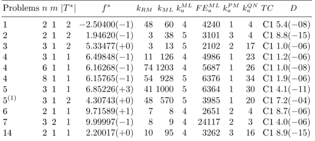
Tables 3 and 4 report on the numerical results obtained by the reduction method combined withE∞ andnk = 1andnk= 5, respectively.
Here we describe some modications that we had to introduce in the de-fault values dened above, for example, on the initial approximation and on the stopping tolerances, in order to obtain convergence.
On problem 2, the runs withE1 andE∞,nk = 1, did not converge to the solution reported in the literature.
On problem 4 withn= 6, the algorithm only converged in the case E∞ withnk = 5. For bothE1andE∞, withnk= 1, usingx0= (0,0.5,0,0,0,0)T, the algorithm found the solution reported in [1]. In one of these runs we had to increase the tolerance ǫg to 10−3. For the run with E1 and nk = 5, an increase ofǫDE to10−4solved the problem.
To be able to converge to the solution of problem 5 with both merit func-tions andnk= 5, the following initial approximation(0.5,0.5,0)and stopping tolerancesǫDE= 10−3 andǫg= 10−2 had to be used.
When solving problems 4 withn= 6 (E∞, nk = 1) and 5 (E∞, nk = 5) with the default values, we observed that although the components ofxwere
not changing in the rst four decimal places the stopping criterion C1 was not satised and from a certain point on the algorithm starts to diverge. This is probably due to the Maratos eect.
Finally, on problem 1 (E1andE∞, withnk= 1) relaxingǫgto10−4makes the termination criterion C1 to be satised.
Details of the corresponding results are reported in the tables.
When the process does not need to recover the rst direction dk,1, the number of iterations of the reduction method equals the number of multi-local optimization calls.
Table 1. Computational results withE1 andnk= 1
Problemsn m|T∗| f∗ k
RM kM L kM La F EaM LkQNa T C D
1 2 1 2 −2.51802(−1) 100 1337 5 2897 3 C27.0(−15)
1(1) 2 1 2 −2.54318(−1) 52 581 5 3062 3 C11.6(−13) 2 2 1 2 4.02110(−1) 7 13 7 4466 5 C18.6(−13)
3 3 1 2 5.33515(+0) 40 41 5 4429 10 C19.3(−06)
4 3 1 2 6.57032(−1) 9 186 5 8576 32 C13.7(−10)
4 6 1 1 1.18871(+1) 100 1070 5 3554 32 C21.4(−03)
4(2) 6 1 2 6.21080(−1) 23 167 5 12137 41 C19.3(−06) 4 8 1 2 6.19758(−1) 7 110 4 3171 36 C12.0(−14)
5 3 1 2 4.43969(+0) 39 181 6 3159 14 C11.8(−07)
6 2 1 1 9.71588(+1) 51 53 4 2958 4 C16.3(−08)
7 3 2 1 9.99999(−1) 45 48 4 24046 4 C17.9(−08)
14 2 1 1 2.22412(+0) 47 173 4 3373 10 C11.1(−12)
(1) -ǫ
g= 10 −4 (2) -x0
= (0,0.5,0,0,0,0)T
Table 2. Computational results withE1 andnk= 5
Problemsn m|T∗| f∗ kRM kM LkM La F EaM LkP Ma kaQN T C D
1 2 1 2 −2.51823(−1) 51 345 5 3065 3 3 C11.4(−07)
2 2 1 2 1.95428(−1) 4 8 5 4214 2 4 C14.8(−13)
3 3 1 2 5.34115(+0) 18 56 5 3390 1 11 C15.9(−10)
4 3 1 2 6.75377(−1) 15 183 5 11180 1 28 C11.2(−10)
4 6 1 1 9.34036(+7) 100 2290 4 3735 1 24 C29.7(+00)
4(1) 6 1 1 6.60021(−1) 84 2084 4 3632 1 22 C12.9(−05) 4 8 1 2 6.28445(−1) 6 47 4 4079 1 39 C15.7(−15)
5 3 1 2 4.30057(+0) 100 1190 5 8092 1 26 C23.8(−03)
5(2) 3 1 2 4.29811(+0) 47 823 5 7112 1 27 C15.1(−04)
6 2 1 1 9.71590(+1) 11 52 4 3343 3 4 C17.0(−09)
7 3 2 1 1.00011(+0) 15 85 4 24130 2 4 C11.2(−07)
14 2 1 1 2.20002(+0) 12 79 4 3268 4 13 C11.6(−09)
(1) -ǫ
DE= 10 −4 (2) -x0
= (0.5,0.5,0)T,
ǫDE= 10 −3
Table 3. Computational results withE∞ andnk= 1
Problemsn m|T∗| f∗ k
RM kM LkaM LF EaM LkQNa T C D
1 2 1 2 −2.52545(−1) 100 377 5 2854 3 C24.9(−11) 1(1) 2 1 2 −2.54386(−1) 61 144 5 3081 4 C11.4(−06) 2 2 1 2 4.76293(−1) 3 38 6 4057 7 C12.7(−13) 2(2) 2 1 2 2.57526(−1) 4 39 6 4324 8 C15.7(−13)
3 3 1 2 5.34326(+0) 21 22 6 5928 10 C11.6(−12)
4 3 1 1 6.76364(−1) 52 573 4 4165 27 C11.4(−07)
4 6 1 1 2.21882(+9) 100 481 4 5871 37 C23.8(+01)
4(3) 6 1 1 6.16754(−1) 25 592 5 3662 32 C13.2(−07) 4 8 1 2 6.18975(−1) 15 157 5 6009 33 C17.4(−13)
5 3 1 2 4.43589(+0) 32 430 6 3616 9 C12.3(−14)
6 2 1 1 9.71589(+1) 44 55 4 2917 4 C14.3(−07)
7 3 2 1 9.99999(−1) 45 48 4 22753 4 C15.3(−07)
14 2 1 1 2.21643(+0) 40 95 4 3158 8 C12.3(−08)
(1) -ǫ
g = 10 −4 (2) -x0
= (−1,0)
T
(3) -x0
= (0,0.5,0,0,0,0)T,ǫ g= 10
−3
Table 4. Computational results withE∞ andnk= 5
Problemsn m|T∗| f∗ k
RM kM LkM La F EaM LkP Ma kaQN T C D
1 2 1 2 −2.50400(−1) 48 60 4 4240 1 4 C15.4(−08)
2 2 1 2 1.94620(−1) 3 38 5 3101 3 4 C18.8(−15)
3 3 1 2 5.33477(+0) 3 13 5 2102 2 17 C11.0(−06)
4 3 1 1 6.49848(−1) 11 126 4 4986 1 23 C11.2(−06)
4 6 1 1 6.16268(−1) 74 1203 4 5687 1 26 C11.0(−08)
4 8 1 1 6.15765(−1) 54 928 5 6376 1 34 C11.9(−06)
5 3 1 1 6.85226(+3) 41 1000 5 6364 1 30 C14.1(−11)
5(1) 3 1 2 4.30743(+0) 48 570 5 3985 1 20 C17.2(−04)
6 2 1 1 9.71589(+1) 7 8 4 2651 2 4 C18.7(−06)
7 3 2 1 9.99997(−1) 8 9 4 24117 2 3 C14.0(−06)
14 2 1 1 2.20017(+0) 10 95 4 3262 3 16 C18.9(−15)
(1) -x0
= (0.5,0.5,0)T,
ǫDE= 10 −3
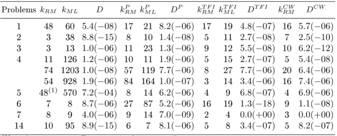
4.2 Comparison with other reduction methods
We include Table 5 in order to allow a comparison between our reduction method and other well-known reduction methods. kRM and kM L represent the number of iterations needed by each reduction method and the number of multi-local optimization calls, respectively. The superscripts P, TFI and CW refer to the results obtained by Price [19], Tanaka, Fukushima and Ibaraki [28] and Coope and Watson [1], respectively.
For a straight comparison we include the results of our variant with E∞ andnk = 5under the columns without the superscript. Although the results of problems 2, 3, 6 and 7 are quite satisfactory for an algorithm that relies on a quasi-Newton based method, some improvements may be obtained on the remaining problems if new strategies as explained in the next section are implemented.
Table 5. Numerical results obtained by reduction methods
Problems kRM kM L D kPRM kM LP DP kRMT F I kM LT F I DT F I kCWRM DCW
1 48 60 5.4(−08) 17 21 8.2(−06) 17 19 4.8(−07) 16 5.7(−06)
2 3 38 8.8(−15) 8 10 1.4(−08) 5 11 2.7(−08) 7 2.5(−10)
3 3 13 1.0(−06) 11 23 1.3(−06) 9 12 5.5(−08) 10 6.2(−12)
4 11 126 1.2(−06) 10 11 1.9(−06) 5 15 2.7(−07) 5 5.4(−08)
74 12031.0(−08) 57 119 7.7(−06) 8 27 7.7(−06) 20 6.4(−06)
54 928 1.9(−06) 84 164 1.0(−07) 3 14 3.4(−06) 16 7.4(−06)
5 48(1) 570 7.2(−04) 8 14 6.2(−06) 4 9 6.8(−07) 4 6.9(−06) 6 7 8 8.7(−06) 27 87 5.2(−06) 16 19 1.3(−18) 9 1.1(−08)
7 8 9 4.0(−06) 9 14 7.0(−09) 2 4 0.0(+00) 3 0.0(+00)
14 10 95 8.9(−15) 6 7 8.1(−06) 5 8 3.4(−07) 5 8.2(−07)
(1) -x0
= (0.5,0.5,0)T,
ǫDE= 10−
3
,ǫg= 10−
2
5 Conclusions and future work
The multi-local algorithm herein presented turns out well in detecting mul-tiple solutions of a nite problem, although we are not able to guarantee that all required solutions are detected. It came to our knowledge that Topological Degree theory [15] may be used to obtain information on the number as well as the location of all the solutions.
It has been recognized that the choice of the penalty parameter value at each iteration,µk, is not a trivial matter. In particular with the two proposed exponential merit functions we have observed that a slight increase in its value rapidly generates some instability. We feel that this problem may be solved using a lter technique that has been proven to be ecient in the nite case [4].
Although our computed solutions can be considered reasonable it remains to be proven that a feasible point that is a critical point to the two merit functions used in this paper also is a stationary point of SIP. Another issue that should be addressed in the future is concerned with the inclusion of a second order correction to prevent the Maratos eect from occurring [14].
Acknowledgments
The authors wish to thank two anonymous referees for their careful reading of the manuscript and their fruitful comments and suggestions.
This work has been partially supported by the Algoritmi Research Center and by Portuguese FCT grant POCI/MAT/58957/2004.
References
1. I. D. Coope and G. A. Watson, A projected Lagrangian algorithm for semi-innite programming, Mathematical Programming 32 (1985), 337356. 2. A. Corana, M. Marchesi, C. Martini, and S. Ridella, Minimizing multimodal
functions of continuous variables with the "simulated annealing" algorithm, ACM Transactions on Mathematical Software 13 (1987), no. 3, 262280. 3. A. Dekkers and E. Aarts, Global optimization and simulated annealing,
Mathe-matical Programming 50 (1991), 367393.
4. R. Fletcher and S. Leyer, Nonlinear programming without a penalty function, Mathematical Programming 91 (2002), 239269.
5. G. Gramlich, R. Hettich, and E. W. Sachs, Local convergence of SQP methods in semi-innite programming, SIAM Journal of Optimization 5 (1995), no. 3, 641658.
6. E. Haaren-Retagne, A semi-innite programming algorithm for robot trajectory planning, Ph.D. thesis, Universitat Trier, 1992.
8. R. Hettich and H. Th. Jongen, Semi-innite programming: conditions of op-timality and applications, Lectures Notes in Control and Information Science, vol. 7, springer ed., 1978, pp. 111.
9. R. Hettich and K. O. Kortanek, Semi-innite programming: Theory, methods and applications, SIAM Review 35 (1993), no. 3, 380429.
10. L. Ingber, Adaptive simulated annealing (ASA): Lessons learned, Control and Cybernetics 25 (1996), no. 1, 3354.
11. H. Th. Jongen and J.-J. Rückmann, On stability and deformation in semi-innite optimization, Semi-Innite Programming (R. Reemtsen and J.-J. Rück-mann, eds.), Nonconvex Optimization and Its Applications, vol. 25, Kluwer Academic Publishers, 1998, pp. 2967.
12. W. B. Kort and D. Bertsekas, A new penalty function method for constrained minimization, In Proceedings of the 1972 IEEE Conference on Decision and Control (1972), 162166.
13. T. León, S. Sanmatías, and H. Vercher, A multi-local optimization algorithm, Top 6 (1998), no. 1, 118.
14. J. Nocedal and S. Wright, Numerical optimization, Springer Series in Operations Research, Springer, 1999.
15. J. M. Ortega and W. C. Rheinboldt, Iterative solution of nonlinear equations in several variables, Academic Press, 1970.
16. K. Parsopoulos, V. Plagianakos, G. Magoulas, and M. Vrahatis, Objective func-tion stretching to alleviate convergence to local minima, Nonlinear Analysis 47 (2001), 34193424.
17. A. I. Pereira and E. M. Fernandes, A study of simulated annealing variants, In Proceedings of the XXVIII Congreso Nacional de Estadística e Investigacion Operativa, ISBN 84-609-0438-5, Cadiz (2004).
18. , A new algorithm to identify all global maximizers based on simulated annealing, Proceedings of the 6th World Congress on Structural and Multidisci-plinary Optimization, J. Herskowitz, S. Mazorche and A. Canelas (Eds.), ISBN: 85-285-0070-5 (CD-ROM) (2005).
19. C. J. Price, Non-linear semi-innite programming, Ph.D. thesis, University of Canterbury, 1992.
20. C. J. Price and I. D. Coope, An exact penalty function algorithm for semi-innite programmes, BIT 30 (1990), 723734.
21. , Numerical experiments in semi-innite programming, Computational Optimization and Applications 6 (1996), 169189.
22. R. Reemtsen and S. Görner, Numerical methods for semi-innite programming: a survey, Semi-Innite Programming (R. Reemtsen and J.-J. Rückmann, eds.), Nonconvex Optimizaion and Its Applications, vol. 25, Kluwer Academic Pub-lishers, 1998, pp. 195275.
23. R. Reemtsen and J.-J. Rückmann (eds.), Semi-innite programming, Nonconvex Optimization and its Applications, Kluwer Academic Publishers, 1998. 24. H. Romeijn and R. Smith, Simulated annealing for constrained global
optimiza-tion, Journal of Global Optimization 5 (1994), 101126.
25. O. Stein, Bi-level strategies in semi-innite programming, Nonconvex Optimiza-tion and Its ApplicaOptimiza-tions, vol. 71, Kluwer Academic, 2003.
27. Y. Tanaka, M. Fukushima, and T. Ibaraki, A comparative study of several semi-innite nonlinear programmnig algorithms, European Journal of Operations Re-search 36 (1988), 92100.
28. , A globally convergence SQP method for semi-innite non-linear opti-mization, Journal of Computational and Applied Mathematics 23 (1988), 141 153.
29. A. I. F. Vaz, E. M. G. P. Fernandes, and M. P. S. F. Gomes, Discretization methods for semi-innite programming, Investigação Operacional 21 (2001), 37 46.
30. G. A. Watson, Globally convergent methods for semi-innite programming, BIT 21 (1981), 362373.