Models
Imen Ghattassi
∗Nour Meddahi
Banque de France Toulouse School of Economics
April 30, 2012
Abstract
The main goal of the paper is to characterize the impact of temporal aggregation on the estimation of the preference’s parameters of a representative agent in a consumption based asset pricing model (CCAPM). We assume that the true economy is at a high frequency (say monthly), that is we model the endowments and the preference of representative agent and then we characterize the asset prices at the high frequency. We then assume that the econometrician observes data at a lower frequency (say annual) and he postulates a model for the endowments and the preferences at the high frequency and he uses the data (implied by the high frequency economy) to estimate the parameters of the model at the low frequency. We are then able to characterize the mapping between the preference’s parameters at low frequency with those of the high frequency. This mapping is analytical in many examples. The model is misspecified at a low frequency, therefore the estimated parameters will depend on the statistical method and the moments that are matched. We therefore follow the CCAPM literature by focusing on matching the means of the risk free rate and the excess returns.
Key Words: Consumption–based asset pricing models, Preferences parameters, decision interval, time–aggregation
JEL Class.: G12, E21, C68
∗Corresponding author: Banque de France, Financial Economics Research Service (DGEI DEMFI
-RECFIN), 31 rue Croix des Petits Champs, 75049 Paris Cedex 01. Tel.: 00 33 (0)1 42 92 49 65. Email: [email protected]
1
Introduction
Asset market data ought to contain valuable information about both investors’ behavior and the sources of systemic and macroeconomic risks that concern investors and hence drive asset markets. Consumption–based asset pricing models (C)CAPM provide a good theoretical tool to access simultaneously the effects of sources of systemic risks and pref-erences.
Following the seminar paper of Lucas (1978), a large theoretical literature has been de-voted to develop (C)CAPM models with different and fully specified endowment process and preferences to replicate a large set of empirical asset pricing facts (the high equity premium, the low risk free rate, the predictability of the price–dividend ratio and the shape of the real and nominal term structure curves...). Typically, the (C)CAPM models proposed in the literature differ by (i) the specification of preferences, (ii) the specification of the state variables, (iii) the interval decision of the consumer or/and (iv ) the sampling interval at which the model is empirically evaluated. Kocherlakota (1996), Campbell (2003) and Cochrane (2007) provide a thorough survey of this literature. For instance, Campbell and Cochrane (1999) solved for equilibrium asset prices in a (C)CAPM with habit formation and when the endowment growth rate follows an i.i.d process. They evaluated the model at monthly frequency and then conducted annual asset pricing mo-ments. Wachter (2006) applied the Campbell and Cochrane (1999) model to access its term structure implications. However, the model was evaluated at quarterly frequency. Piazzesi and Schneider (2006) provided solutions for the equilibrium yield curves under the assumptions of recursive preferences and a state-space specifications of both consump-tion growth rate and inflaconsump-tion. The model was evaluated at quarterly frequency. Bansal and Yaron (2004) developed a long–run risks (LRR) asset pricing model with recursive preferences and when the consumption growth rate presents both predictable and uncer-tainty components. They calibrated the model at monthly frequency. In Bansal, Kiku and Yaron (2010), the long–run risks model was estimated using annual financial and macroeconomic data and assuming that the decision interval of the consumer is monthly. They also evaluated empirically the effects of ignoring the time–aggregation if the decision interval was annual.
In this paper, we propose a tractable analytical tool to evaluate the effects of (i) ignoring time–averaging and/or (ii) misspecified state variables or preferences. Without loss of generality, we first assume that the decision interval is monthly. We solve for the con-sumer maximization program. Then, we assume that the econometrician observes annual data and believes that the decision interval of the consumer is annual. Therefore, the
asset pricing implications of the consumer model and the monthly state variables are aggregated at annual level. Based on the consumer and the econometrician programs, we provide the analytical relationship between the monthly preferences parameters of the consumer (ignored by the econometrician) and the annual preferences parameters (that the econometrician manages to estimate) that provide the same unconditional means of the risk–free rate and the equity premium. Thanks to our analytical formulas, we are able to conduct a thorough comparative analysis between models by taking different special cases of (i) the utility function or/and (ii) the law of motion of the endowment growth process and by taking small variations in preferences parameters.
On the empirical side, we evaluate the effects of ignoring time–aggregations on two classes of (C)CAPM models: (i) the (C)CAPM model with separable preferences and i.i.d en-dowment process and (ii) the long–run risks model of Bansal and Yaron (2004). We show that relationship between monthly and annual preferences parameters deeply depends on the specification of the state variables and the utility function.
Note that having an analytical formula will make it a lot easier to study the empirical investigation of others classes of (C)CAPM models. Moreover, our theoretical framework allows us to extend our theoretical and empirical works to a larger set of moments for returns, namely the standard deviation of the equity premium and the risk–free rate and the mean and the volatility of the price–dividend ratio.
2
Consumption, Asset Returns Moments, and
Time-Aggregation
The goal of the present section is to characterize the link between the moments of con-sumption growth at monthly and annual frequencies, as well those of financial variables like the risk-free rate and the excess returns. The connection from a frequency to another one of these moments will play a central role in the paper.
2.1
Temporal Aggregation Effects on Consumption Growth
Let Cm,t and ∆cm,t = log
³
Cm,t
Cm,t−1
´
denote the monthly consumption and the monthly consumption growth at date t respectively.
We assume that the econometrician only observes consumption data at annual frequency. Annual consumption Ca,12t at date 12t is defined as the sum of monthly consumptions
spanning the period from 12(t − 1) to 12t, that is, Ca,12t=
P11
i=0Cm,12t−i. It follows that
the annual consumption growth ∆ca,12t= log
³
Ca,12t
Ca,12(t−1)
´ .
Following Bansal, Kiku and Yaron (2007), we log-linearize the annual consumption growth around the expected values of each month consumption growth and we get:
∆ca,12(t+1)∼=
23 X
i=0
τi∆cm,12(t+1)−i (1)
where τi,i=0,...,23, are given by:
τi = Pi m=0exp ¡ (12 − m)∆cm ¢ P11 j=0exp ¡ (12 − j)∆cm ¢ if i < 12 P11 j=0exp ¡ (12 − j)∆cm ¢ −Pi−12m=0exp¡(12 − m)∆cm ¢ P11 j=0exp ¡ (12 − j)∆cm ¢ if i ≥ 12 (2)
where ∆cm is the unconditional1mean of the monthly consumption growth. See Appendix
A for a proof of Eq. (1).
Observe that Bansal, Kiku and Yaron (2007) did their log-linearization around zero, i.e., they imposed ∆cm = 0 in (1), which leads to:
τi = i + 1 12 if i < 12 23 − i 12 if 12 ≤ i ≤ 23 (3)
Likewise, Eq. (1) nets the naive case
∆ca,12t=
11 X
i=0
∆cm,12t−i,
corresponding to τi = 121 for 0 ≤ i ≤ 12 and 0 otherwise, where one would assume wrongly
that the annual growth of consumption equals the sum of the monthly consumption growths. We will consider this example later.
We will now assess the precision of Eq. (1) when the consumption monthly growth is assumed to be i.i.d. N (µc,m, σc,m2 ). We study later the long-run risk case. Under the i.i.d.
assumption of monthly consumption growth, Eq. (1) implies that the annual growth is
an MA(1) process with µc,a= Ã 23 X i=0 τi ! µm,c = 12µm,c (4) σ2c,a= Ã 23 X i=0 τi2 ! σ2m,c. (5)
Likewise, the normality assumption of monthly consumption growth combined with Eq. (1) imply that the annual consumption growth is normal.
The assessment of the precision of Eq. (1) is done by simulations. We consider the parameters values considered in Bansal, Kiku, and Yaron (2007) for the monthly con-sumption return, that is µc,m = 0.15% and σc,m = 0.55% and simulate 1,000 replications
of samples with size equal to 10,000. We consider such long size because we are interested in characterizing the aggregation’s impact in population and not in finite sample. The simulations results give µc,a= 1.80001% and σc,a = 1.557646% while Eq. (1) implies that
µc,a= 1.8% whether one uses Eq. (2) or Eq. (3), while one gets σc,a = 1.558338% under
Eq. (2) and σc,a = 1.558334% Eq. (3). Consequently, we can conclude that Eq. (1) is a
good approximation, and that using Eq. (2) or Eq. (3) lead to the same results. We will study in a revised version the quality of the MA(1) and normality properties of annual consumption growth.
2.2
Temporal Aggregation Effects on Asset Returns Moments
Let rfm,t = log ³
1 + Rfm,t ´
denote the monthly real risk–free rate (that pays for sure one unit of consumption at next month) and ra,12tf = log
³
1 + Rfa,12t ´
the corresponding annual real risk–free rate. It follows that:
ra,12tf = 11 X
i=0
rfm,12t−i (6)
The monthly (gross) return (1 + R(j)m,t) of a risky asset j that pays the monthly dividend D(j)m,t between t − 1 and t is defined as follows:
1 + R(j)m,t = P (j) m,t+ D (j) m,t Pm,t−1(j)
where Pm,t(j) denotes the corresponding monthly price. If monthly dividends are assumed to be reinvested within the annual period, therefore, the annual dividend D(j)a,12t
corre-sponding to the period 12(t − 1) and 12t verifies Da,12t(j) = D(j)m,12t+ 11 X i=1 Dm,12t−i(j) Ã i Y j=1 R(j)m,12t+1−j !
It implies that the annual (log) return of the risky asset (j) ra,12t(j) = 11 X i=0 r(j)m,12t−i (7) Let rc
m,t denote the (log) return of the unobservable market portfolio that pays off
con-sumption. We assume that the corresponding annual (log) return ra,12t is derived as
follows: ra,12t(c) = 11 X i=0 r(c)m,12t−i (8)
It is worth noting that at this stage, no specification is imposed to the variables of interest. Relations (1), (6), (7) and (8) are valid what ever the law of motion of the monthly consumption growth, the monthly risk–free rate or the monthly return of the market portfolio.
3
Asset-pricing with CRRA preferences and log–normal
consumption growth
In this section, we assess the effect of time-aggregation on asset pricing models when preferences are time–separable and the consumption growth is a log–normal i.i.d process. We assume that the decision interval of the agent and the sampling frequency of the data do not coincide. Without loss of generality, we assume that the decision interval of the agent is monthly and the actual data are sampled annually. Therefore, the consumer decisions are derived at monthly frequency but the asset pricing model is evaluated at annual frequency.
In the following we first present the monthly program of the consumer by assuming that his decisions are derived from a Consumption–based Asset pricing Model with power utility and i.i.d log–normal consumption growth. It is the benchmark model in the (C)CAPM literature in which asset prices and expected returns can be found in closed form. Then we analyze the econometrician program at annual frequency.
3.1
the consumer program
At monthly frequency, we assume that the consumer determines his contingent monthly consumption (Cm,t)∞t=0 plan by maximizing his inter–temporal expected utility function:
Et P∞ s=0δms Cm,t+s1−γm−1 1−γm if γm 6= 1 Et P∞ s=0δms log (Cm,t+s) if γm = 1
subject to his budget constraint:
Wm,t+1= (Wm,t− Cm,t)Rm,t+1c
where Wm,t denotes the monthly total wealth of the agent and Rcm,t is the return on all
invested wealth.
The parameter 0 < δm < 1 is the agent’s monthly time preferences and the parameter γm
is the monthly coefficient of risk aversion. Expectations are conditional on information available at beginning of date t. The first–order condition that determines the agent’s consumption choices is given by the following Euler equation:
Et= [Mm,t+1Ri,t+1]
where Ri,t+1is the gross return of any asset i and Mm,t+1is the monthly stochastic discount
factor given by:
mm,t+1 = log (Mm,t+1) = exp (log(δm) − γm∆cm,t+1)
The monthly consumption growth is assumed to follow a log–normal i.i.d process:
∆c(m)t+1 = µ(m)+ σ(m)²t+1
where ²t∼ N(0, 1).
Therefore, the unconditional mean of the monthly risk free rate is given by:
r(m)f = − log δ(m)+ γ(m)µ(m)− ¡
γ(m)σ(m)¢2
2 (9)
and the unconditional mean of the equity premium2 is er(m) = E ³ ert(m) ´ = E ³ rc,t(m) ´ − E ³ r(m)f,t ´ = (γm− 1 2)(σ (m))2 (10)
2Compared to the well-known formula er = γσ2, the equity premium (10) presents an additional term 1
2
¡
The proof is presented in Appendix B.
3.2
The econometrician program
The econometrician observes annual consumption growth data ∆ca,12t and assumes that
the consumption decisions of the representative agent are annual. In other words, he assumes that the consumer derives his annual contingent consumption each year by max-imizing his annual utility function:
E12t P∞ s=0δas Ca,12(t+s)1−γa −1 1−γa if γa6= 1 E12t P∞ s=0δas log ¡ Ca,12(t+s) ¢ if γa= 1
subject to his annual budget constraint:
Wa,12(t+1)= (Wa,12t− Ca,12t)Rca,12(t+1)
where the parameter δa is the agent’s annual time preferences and the parameter γa is
the annual coefficient of risk aversion. Wa,12(t+1)and Rca,12tdenote respectively the annual
wealth of the agent accumulated during the period between 12t and 12(t + 1) and the an-nual return on all invested wealth. Expectations are conditional on information available at the beginning of the annual date 12t. The econometrician derives the corresponding annual asset pricing Euler conditions to evaluate the annual preferences parameters:
E12t h
exp(ma,12(t+1)+ ra,12(t+1)j )
i
= 1 (11)
where ra,12(t+1)j is the log of the annual gross return on asset j and ma,12(t+1)is the annual
(log) inter–temporal marginal rate of substitution defined as follows:
ma,12(t+1)= log δa− γa∆ca,12(t+1) (12)
To solve for the annual Euler equation, the econometrician needs to specify the low of motion of the annual consumption growth. As explained above, the annual consumption growth is generated by Equation (1). Based on this relation, the annual consumption growth follows an MA(1) process when the monthly consumption growth follows a log-normal i.i.d process. But, to better understand the effects of ignoring time–aggregation, three cases are under investigation. First, we assume that the econometrician believes that the annual consumption growth follows an lognormal i.i.d process with a wrong vari-ance. Second, we assume that the econometrician observes the right variance of annual
consumption growth but continues to believe that the annual consumption growth follows an lognormal i.i.d process. Finally, the econometrician assumes the right law of motion of annual consumption growth.
3.2.1 Case 1
We assume that the econometrician builds the annual consumption growth as follows ∆ca,12t =
11 X
i=0
∆cm,12t−i
This specification can be expressed as in the general specification (1) described in the pervious section when aggregation coefficients (τi)i=0:23 verify:
(
τi = 1 if i ≤ 11
0 otherwise
It implies that the annual consumption growth follows an i.i.d process where: µc,a = E (∆ca,12t) = 12µc,m
and
σ2
c,a= V ar (∆ca,12t) = 12σ2c,m
Therefore, the annual unconditional means of risk free rate and equity premium are rf,t(a)= −log(δa) + 12γaµ(m)− 12 ¡ γ(a)σ(m)¢2 2 (13) and er(a) = 12(γ a− 1 2)(σ (m))2 (14)
Relations (6), (8), (9), (10), (13) and (14) imply the following proposition:
Proposition 1 We assume that monthly consumptions are generated by a Consump-tion Asset Pricing Model with time–separable preferences with Gaussian i.i.d endow-ment growth process. Let δm and γm denote the monthly coefficients of subjective time–
preference and risk aversion respectively and µm and σ2m denote the unconditional mean
and variance of consumption growth process.
The econometrician believes that the decision interval of the consumer is annual rather than monthly. He estimates annual preferences parameters δa and γa by assuming that (i)
i.i.d process with mean equal to 12µm and variance equal 12σ2m. Therefore, the theoretical
preferences parameters δa and γa to be estimated are
δa = δm12 (15)
γa = γm (16)
Equations (15) and (16) derive the theoretical annual parameters that the econometrician should estimate under the assumptions of Proposition 1. Two main results emerge. First, Eq. (16) shows that the coefficient of risk aversion is unchanged what ever the sampling interval. If the econometrician estimates the coefficient of risk aversion using the asset pricing implications of the annual model rather than the true monthly model, there is no estimation bias related to the time–aggregation effects. As we can see later, this is the only case when the misspecification of the decision interval of the consumer does not matter. Second, the relation between the annual and the monthly subjective discount factor is unchanged what ever the values of monthly coefficient of risk aversion. Indeed, we found the well-used relationship δa= δm12.
3.2.2 Case 2
The econometrician observes the true actual annual consumption data, but he continues to believe that the annual consumption growth is i.i.d. It implies that
µc,a = E (∆ca,12t) = 12µc,m and σ2 c,a= V ar (∆ca,12t) = σc,m2 Ã 23 X i=0 τ2 i ! = 12α2σ2 c,m where α2 = 1 12 P23
i=0τi2. Following the same methodology, we obtain the following mapping
from monthly to annual preference parameters:
Proposition 2 We assume that monthly consumptions are generated by a Consump-tion Asset Pricing Model with time–separable preferences with Gaussian i.i.d endow-ment growth process. Let δm and γm denote the monthly coefficients of subjective time–
preference and risk aversion respectively and µm and σ2m denote the unconditional mean
and variance of consumption growth process.
The econometrician believes that the decision interval of the consumer is annual rather than monthly. He estimates annual preferences parameters δa and γa by assuming that
gaussian i.i.d process with mean equal to 12µm and variance equal 12α2σ2m. Therefore,
the theoretical preferences parameters δa and γa to be estimated are
δa = δm12+ (2γm− 1)(1 − α2) 2α2 µc,m+ σ 2 c,m µ γ2 m− (2γm− 1 + α2)2 4α2 ¶ (17) γa = 2γm− 1 + α2 2α2 (18)
By setting α2 = 1, we recover Proposition1. Some numerical results are reported in Table (1).
[ Table 1 about here ]
Two main results emerge. First, the monthly subjective discount factor does not affect the annual value of the risk aversion coefficient. For example, if the monthly coefficient of risk aversion γm is egal to 5, the annual γa is always equal to 7.22 what ever the value
of γm. Moreover, the annual γa is more than 40% greater than the corresponding γm. For
instance, when γm is equal to 20, the corresponding γais equal to 29.64%. Second, even if
the theoretical relation 17implies that the annual subjective discount factor depends on both δm and γm, the numerical results shows that is that the annual subjective coefficient
βa is always an increasing function of the monthly risk aversion coefficient γm.
3.2.3 Case 3
The econometrician observes the true actual annual consumption data and believes that the annual consumption growth follows a MA(1) process:
∆ca,12(t+1) = µc,a+ Θζ12t+ ζ12(t+1)
where µc,a = 12µc,m denote the unconditional mean of annual consumption growth. Based
on Equation (1), the variance of annual consumption growth rewrites
σ2
c,a= 12α2σ2c,m = (1 + Θ2)σζ2
Following the same methodology used to solve the cases 1 et 2 and applying the implicit functions theorem, we derive the following mapping from monthly to annual preferences:
Proposition 3 We assume that monthly consumptions are generated by a Consump-tion Asset Pricing Model with time–separable preferences with Gaussian i.i.d endow-ment growth process. Let δm and γm denote the monthly coefficients of subjective time–
preference and risk aversion respectively and µm and σ2m denote the unconditional mean
and variance of consumption growth process.
The econometrician believes that the decision interval of the consumer is annual rather than monthly. He estimates annual preferences parameters δa and γa by assuming that
(i) the annual utility function is CRRA and (ii) the annual consumption growth follows a gaussian MA(1) process with mean 12µc,m, variance 12α2σc,m and lagged moving–average
coefficient Θ. Therefore, the theoretical preferences parameters δa and γa to be estimated
are δa = δa0− (Θδ0 a) 2¡ 12µc,m− 12γa0α2σ2c,m ¢ 6α2σ2 c,m exp¡12(1 − γ0 a)µc,m+ 6(1 − γ0)2α2σc,m2 ¢ (19) γa = γa0− Θβ0 a 6α2σ2 c,m exp¡12(1 − γa0)µc,m+ 6(1 − γ0)2α2σc,m2 ¢ (20) where δ0
a and γa0 correspond to the case when Θ = 0.
Appendices C and D provide more technical details. By setting Θ = 0, we recover Proposition2. Some numerical results are presented in Table 2.
[ Table 2 about here ]
As we can see in this table, the behavior of annual subjective discount factor and the risk aversion coefficient are completely different from the previous cases. Indeed, the βa is a
decreasing function of the monthly risk aversion coefficient. Moreover, βa is always low
than the corresponding βm. In the second side of the Table 2, the annual risk aversion
coefficient is low what ever the value of the monthly risk aversion coefficient. For instance, when the monthly risk aversion is equal to 20, the corresponding annual parameter does not exceed 4.48.
4
(C)CAPM models with Epstein-Zin preferences and
Affine State Variables
In the following we first present the monthly program of the consumer by assuming that his decisions are derived from a Consumption–based Asset pricing Model with recursive
preferences and when the exogenous state variables follow affine processes as in Eraker (2008). Then ,we analyze the econometrician program. Finally, we present some empirical results to evaluate the impact of time–aggregation.
4.1
The theoretical framework
4.1.1 The consumer program
Following Bansal and Yaron (2004), we consider a representative agent when the prefer-ences are defined recursively as follows:
Vm,t = · (1 − δm)C 1−γm θm m,t + δm ¡ Et £ V1−γm m,t+1 ¤¢ 1 γm ¸ θm 1−γm (21) where 0 < δm < 1 is the agent’s monthly time preferences, the parameter γmis the monthly
coefficient of risk aversion, the parameter ψm is the monthly elasticity of intertemporal
substitution and the parameter θm = 1−1−γ1m
ψm
. Expectations are conditional on information available at beginning of date t.
Each month, the consumer determines his contingent monthly consumption plan {Cm,t}∞0 by maximizing his life–time utility (21) subject to the budget constraint.
Hence, agents’ consumption decisions are governed by the following (log) inter–temporal marginal of substitution:
mm,t+1= θmlog δm−
θm
ψm
∆cm,t+1+ (θm− 1)rcm,t+1 (22)
Therefore, for any asset j, the first order condition of the agent maximization program yields the following asset pricing equation:
Et
£
exp(mm,t+1+ rjm,t+1)
¤
= 1 (23)
where rjm,t+1 is the (log) ) monthly gross return on asset j.
To solve the pricing formulas (23), we need to specify the law of motion of the endowment growth process. The monthly consumption growth is assumed to be linear function of the monthly state variable Xm,t of dimension s:
∆cm,t = x0m,cXm,t (24)
The state variable Xm,t is assumed to follow un affine process, defined by the following
affine conditional Laplace transform function: Et ³ exp z0Xm,t+1 ´ = exp(a0(z)X m,t+ b(z)) (25)
where a(z) 6= 0 for any multi–variable z with complex components, such that the condi-tional expectation exists.
As the state variable is assumed to be exogenous, the functions a(z) and b(z) are known explicitly. It is worth noting that the general class of affine processes nests some endow-ments environendow-ments proposed in the (C)CAPM models as in Campbell and Cochrane (1999), Piazzesi and Schneider (2006) and Bansal and Yaron (2004), among others. As discussed in Bansal, Kiku and Yaron (2010), one needs to solve for the unobservable return on total wealth to characterize the inter–temporal marginal rate of substitution. Therefore, we use the Campbell and Shiller (1988) approximation to solve for rc
m,t: rc m,t+1= km,0+ km,1zm,t+1+ ∆cm,t+1− ∆cm,t (26) where zm,t = log ³ Pm,t Cm,t ´
is the (log) monthly price–consumption ratio and km’s are
con-stants of log–linearization, defined by Campbell and Shiller (1988) as follows: km,1 = exp(zm)
1 + exp(zm)
(27) km,0 = log (1 + exp(zm)) − km,1zm (28)
The parameter zmdenote the unconditional mean of the the (log) monthly price–consumption
ratio.
Given the approximation (26), we require a solution for the price–consumption ratio zm,t
to derive the solution for rc m,t+1.
We consider the following form for the solution zm,t:
zm,t = zm,0+ zm,10 Xm,t (29)
where zm,0 is a scalar and zm,1 is a (s ∗ 1) vector. The solution parameters zm’s are
determined by the following Euler condition: Et
£
exp(mm,t+1+ rcj,t+1)
¤
= 1 (30)
The solution for the parameters zm’s depend on (i) the monthly preferences parameters,
(ii) the parameters that govern the dynamics of the monthly consumption growth and (iii) the unconditional mean of the (log) price–consumption ratio zm.
In order to solve for zm, we solve numerically the following fixed-point problem:
zm = Zm(z)Xm
where Xm is the unconditional mean of the monthly state variable Xm,t.
The asset pricing problem is solved numerically and we obtain the solution of zm as
function of the monthly preferences parameters (δm, γm, ψm) and the parameters that
governs the dynamics of monthly consumption growth (a(.), b(.)): zm = zm(δm, γm, ψm, xm,c, a(.), b(.))
More details are provided in appendix E.
It follows that the unconditional mean for the (log) gross monthly return on total wealth is given by:
rcm = km,0+ km,1zm+ ∆cm− zm (31)
The (log) monthly risk free rate rfm,t+1 is known at date t and verifies:
Et
h
exp(mm,t+1+ rfm,t+1)
i
= 1 (32)
Using the approximation (26), the solution for the coefficients zm’s and the solution for
the unconditional mean zm , we obtain the solution for the unconditional mean of the
(log) monthly risk free rate:
rfm = −θmlog δm+ (1 − θm)km,0+ (θm− 1)(1 − km,1)zm,0− b µµ θm− 1 − θm ψm ¶ xcm,c+ (θm− 1)km,1zm,1 ¶ (33) + µ (θm− 1)zm,1− a0 µµ θm− 1 − θm ψm ¶ xm,c+ (θm− 1)km,1zm,1 ¶¶ Xm (34)
4.1.2 The econometrician program
The econometrician observes data at annual frequency. Let Xa,12tdenote the annual state
variable defined as follows:
Xa,12t= Xm,12t Xm,12t−1 . . . Xm,12t−23 Therefore, the annual consumption growth rewrites:
∆ca,12(t+1) = x0a,cXa,12(t+1) (35)
where x0
a,c= [ τ0x0m,x τ1x0m,x ... τ23x0m,x ].
It is worth noting that the annual state variable Xa,12t follows an affine process
charac-terized by the following affine conditional Laplace function: E12t
£
exp¡u0X
a,12(t+1)
¢¤
= [exp (A(u)Xa,12t+ B(u))] (36)
where the functions A(u) and B(u) are specified in Appendix D.
The econometrician observes annual consumption growth data ∆ca,12t and assumes that
the consumption decisions of the representative agent are annual. In other words, he assumes that the consumer derives his annual contingent consumption each year by max-imizing his annual utility function:
Va,12t= · (1 − δa)C 1−γa θa a,12t + δa ³ E12t h V1−γa a,12(t+1) i´ 1 γa ¸ θa 1−γa (37) subject to his annual budget constraint:
Wa,12(t+1)= (Wa,12t− Ca,12t)Rca,12(t+1)
where the parameter δa is the agent’s annual time preferences, γa is the annual coefficient
of risk aversion, θa = 1−1−γ1a
ψa and ψa is the annual elasticity of intertemporal substitution.
Wa,12(t+1)and Ra,12tc denote respectively the annual wealth of the agent accumulated
dur-ing the period between 12t and 12(t + 1) and the annual return on all invested wealth. Expectations are conditional on information available at beginning of the annual date 12t. As explained above, the annual consumption growth is generated by Equation(35).
The econometrician derives the corresponding annual asset pricing Euler conditions to evaluate the annual preferences parameters:
E12t h
exp(ma,12(t+1)+ ra,12(t+1)j )
i
= 1 (38)
where ra,12(t+1)j is the log of the annual gross return on asset j and ma,12(t+1)is the annual
(log) intertemporal marginal rate of substitution defined as follows: ma,12(t+1)= θalog δa−
θa
ψa
∆ca,12(t+1)+ (θa− 1)rca,12(t+1) (39)
Following the same methodology used below to solve for the monthly asset pricing prob-lem, we derive the unconditional means of annual return on the total wealth invested and annual risk free rate. It implies that:
rc
a= ka,0(za) + (ka,1(za) − 1) za+ ∆ca
and rf
a = −θalog δa+ (1 − θa)ka,0+ (1 − θa)(ka,1− 1)Za,0− B
µµ θa− θa ψa − 1 
xa,c+ ka,1(θa− 1)Za,1
¶ (40) + µµ 1 − θa+ θa ψa ¶ x0a,c− A0 µµ θa− θa ψa − 1 ¶ x0a,c+ (θa− 1)Za,10 ¶¶ Xa (41)
4.2
Concrete case: Long Run Risks Model of Bansal and Yaron
(2004)
The long–run risks model of Bansal and Yaron (2004) is a special case of (C)CAPM model with Epstein-Zin preferneces and affine state variables. Indeed, in Bansal and Yaron (2004) model, preferences are assumed to be recursive and the monthly consumption growth process is evolving dynamically as follows:
∆cm,t+1= g∆cm+ xm,t+ σm,tηm,t+1
xm,t+1= ρmxm,t+ ϕm,eσm,tem,t+1
σ2
m,t+1= σ2m+ νm,1(σ2m,t− σ2m) + σm,wwm,t+1
xm,t presents the persistent predictable component and σm,t the time–varying economic
uncertainty incorporated in monthly consumption growth rate. The parameters of the Long Run Risk model are set as follows:
∆cm = 0.0015 ρm = 0.979 ϕm,e= 0.038 σm = 0.0072 νm,1 = 0.987 σm,w = 0.28E(−5)
The consumption growth rate can be written as a linear combination of affine state vari-ables when
• the state variable Xm,t =
h ∆cm,t xm,t σm,t2 i ’ • xm,c= [1 0 0]’ • a(z) = z0 0 1 0 0 ρm 0 0 0 νm,1 +12z0 diag¡1, ϕ2 m,e, 0 ¢ z 0 0 1 0 • b(z) = z0 g∆cm 0 (1 − νm,1)σm2 + 12z0 diag(0, 0, σ m,w)z
To assess the effects of time–aggregation, two cases are under investigation.
• case 1: we assume that the econometrician believes that the law of motion of the consumption growth is stable over time. Therefore, at annual frequency, the consumption growth follows the same LRR process with annual coefficients:
∆ca,12(t+1) = g∆ca+ xa,12t+ σa,12tηa,12(t+1)
xa,12(t+1) = ρaxa,12t+ ϕa,eσa,12tea,12(t+1)
where ea,12t, ηa,12t and wa,12t ; N.i.i.d(0, 1).
Following Bansal, Kiku and Yaron (2010), the model is calibrated as follows:
ρa = 0.9422
ϕa,e = 0.0645
σa = 0.00235
νa,1 = 0.9593
σa,w = 0.72E(−5)
• case 2: we assume that the econometricians observes the exact low of motion of the annual consumption growth that tabes into account aggregation effect and that is derived from the equation (36).
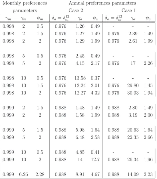
Empirical results of cases 1 and 2 are reported in Table (3). For every set of monthly preferences parameters (γm, γm, ψm), we report the corresponding annual preferences
parameters (γa, γa, ψa). As a starting point, we assume that δa = δm12. The main result
that emerges is the following: if the econometricians ignores time–aggregation, then higher annual risk aversion coefficients are needed to replicate the same unconditional means of risk free rate and equity premium. for instance, when δm, γm and ψm are set to 0.999,
10 and 2, the annual coefficients of risk aversion under the cases 1 and 2 are respectively 26.34 and 14.
Table 1: Case 2
δ
aγ
a γm\ δm 0.95 0.98 0.985 0.99 0.999 γm\ δm 0.95 0.98 0.985 0.99 0.999 2 0.541 0.785 0.834 0.887 0.988 2 2.74 2.74 2.74 2.74 2.74 5 0.542 0.786 0.836 0.888 0.990 5 7.22 7.22 7.22 7.22 7.22 7 0.543 0.787 0.837 0.889 0.991 7 10.21 10.21 10.21 10.21 10.21 10 0.544 0.788 0.838 0.890 0.992 10 14.70 14.70 14.70 14.70 14.70 15 0.545 0.790 0.839 0.891 0.993 15 29.64 29.64 29.64 29.64 29.64 δm 0.540 0.784 0.83 0.88 0.98Note: This table reports the relationship between monthly preferences parameters (γm,γm) and
an-nual preferences parameters γa and γa (i) when the monthly dynamic generating process of
finan-cial data is monthly and based on a Consumption–based asset model with power utility function
Um,t = Et
P∞
i=0(δm)i C 1−γm
m,t+i−1
1−γm and i.i.d consumption growth rate ∆cm,t = µc,m+ σc,m²m,t and (ii)
when the econometrician estimates the model at annual frequency by assuming that the annual prefer-ences are separable Ua,12t = E12t
P∞
i=0(δa)i C 1−γa
a,12(t+i)−1
1−γa and by misspecifying the annual consumption
growth process ∆ca,12t = 12µc,m+
qP23 i=0τi2σc,m²a,12t. Table 2: Case 3
δ
aγ
a γm\ δm 0.95 0.98 0.985 0.99 0.999 γm\ δm 0.95 0.98 0.985 0.99 0.999 2 0.55 0.79 0.84 0.90 1.00 2 3.84 3.09 2.984 2.88 2.71 5 0.53 0.76 0.80 0.85 0.95 5 3.96 3.18 3.07 2.96 2.79 7 0.51 0.73 0.78 0.83 0.92 7 4.04 3.24 3.13 3.02 2.84 10 0.49 0.70 0.74 0.79 0.88 10 4.15 3.33 3.21 3.10 2.91 20 0.43 0.62 0.66 0.70 0.77 20 4.48 3.59 3.46 3.34 3.14Note: This table reports the relationship between monthly preferences parameters (γm,γm) and
an-nual preferences paremeters γa and γa (i) when the monthly dynamic generating process of
finan-cial data is monthly and based on a Consumption–based asset model with power utility function
Um,t= Et
P∞
i=0(δm)i C 1−γm
m,t+i−1
1−γm and i.i.d consumption growth rate ∆cm,t= µc,m+ σc,m²m,tand (ii) when
the econometrician estimates the model at annual frequency by assuming that the annual preferences are separable Ua,12t = E12t
P∞
i=0(δa)i C 1−γa
a,12(t+i)−1
1−γa and by specifying correctly the annual consumption
Table 3: Long Run Risks model with Recursive Preferences
Monthly preferences Annual preferences parameters
parameters Case 2 Case 1
γm γm ψm δa= δ12m γa ψa δa = δm12 γa ψa 0.998 2 0.5 0.976 1.26 0.49 - - -0.998 2 1.5 0.976 1.27 1.49 0.976 2.39 1.49 0.998 2 2 0.976 1.29 1.99 0.976 2.61 1.99 0.998 5 0.5 0.976 2.45 0.49 - - -0.998 5 2 0.976 4.15 2.17 0.976 17 2.26 0.998 10 0.5 0.976 13.58 0.37 - - -0.998 10 1.5 0.976 12.24 2.01 0.976 29.80 1.45 0.998 10 2 0.976 12.27 4.32 0.976 30.03 1.94 0.999 2 1.5 0.988 1.48 1.49 0.988 2.80 1.49 0.999 2 2 0.988 1.58 1.99 0.988 3.19 2.00 0.999 5 1.5 0.988 5.98 1.64 0.988 20.63 1.64 0.999 5 2 0.988 6.48 2.58 0.988 22.35 2.66 0.999 10 0.5 0.988 4.85 0.41 - - -0.999 10 2 0.988 14 12.7 0.988 26.34 1.96 0.999 6.26 2.28 0.988 8.91 4.67 0.988 14.09 2.23
Note: This table reports the relationship between monthly preferences parameters (ψm,γm) and
an-nual preferences paremeters ψa and γa (i) when the monthly dynamic generating process of
finan-cial data is monthly and based on a Consumption–based asset model with recursives preferences
Vm,t= · (1 − δm)C 1−γm θm m,t + δm ³ Et h V1−γm m,t+1 i´ 1 γm ¸ θm 1−γm
and when the monthly consumption gorowth rate is specified as in Bansal and Yaron (2004).
Bibliography
Bansal, R., Dittmar, R.F. and Lundblad, C., 2005. Consumption, dividends, and the cross section of equity returns, Journal of Finance 60, 1639–1672.
Bansal, R., Gallant, R. and Tauchan, G., 2005. Rational Pessimism, Rational Exuberance and Asset Pricing Models, Working paper, Duke University.
Bansal, R. Khatchatrian, V. and Yaron, A., 2005. Interpretable asset markets?, European Economic Review 49, 531–560.
Bansal, R. and Yaron, A., 2004. Risks for the long run: A potential resolution of asset pricing puzzles. Journal of Finance 59, 1481–1509.
Bansal, R., Kiku, D. and Yaron, A., 2010. Risks for the Long Run: Estimation and Inference. working paper.
Barro, R. J., 2006. Rare Disasters and Asset Markets in the Twentieth Century, Quarterly Journal of Economics, 121:3:823–866.
Campbell, J.Y., 2003. Consumption-based Asset Pricing. In: Constantinides, G., Har-ris, M. and Stulz, R. (Eds.), Handbook of the Economics of Finance. North-Holland, Amsterdam.
Campbell, J.Y. and Cochrane, J.H., 1999. By Force of Habit: A Consumption Based Explanation of Aggregate Stock Market Behavior. Journal of Political Economy 107, 205–251.
Campbell, J.Y. and Shiller, R., 1988. Stock Prices, Earnings and Expected Dividends, Journal of Finance 43, 661–676.
Cochrane, J.H., 2005. Asset Pricing. Princeton University Press.
Cochrane, J.H., 2007. Financial Markets and the Real Economy. Princeton University Press.
Epstein, L.G., Zin, S.E., 1989. Substitution, risk aversion, and the intertemporal behavior of consumption and asset returns: A theoretical framework. Econometrica 57, 937–969. Epstein, L.G., Zin, S.E., 1989. Substitution, risk aversion, and the intertemporal behavior of consumption and asset returns: An empirical framework. Journal of Political Economy 57, 937–969.
Lucas, R., 1978. Asset Prices in an Exchange Economy. Econometrica 46, 1439–1445. Kiku, D., 2006. Long Run Risks and the Value Premium Puzzle, Working paper, The Wharton School, University of Pennsylvania.
Kocherlakota, N.R., 1996. The Equity Premium: It’s Still a Puzzle, Journal of Economic Literature 34(1), 42-71.
Piazzesi, M. and Schneider, M., 2006. Equilibrium Yield Curves, NBER Macroeconomics Annual.
Wachter, J.A., 2006. A Consumption–based Model of the Term Structure of Interest Rates. Journal of Financial Economics 79, 365–399.
Wilcox, D. 1992. The construction of U.S. consumption data: Some facts and their implications for empirical work. American Economic Review 82, 922–941.
A
From Monthly to Annual Consumption Growth
We assume that the time interval is monthly. Let C12(t+1)(a) = P11i=0C12(t+1)−i(m) denote the annual aggregate consumption spanning the period between 12t and 12(t + 1). Therefore, the (log) annual consumption growth at time 12(t + 1) verifies:
∆c(a)12(t+1) = log à C12(t+1)(a) C12(t)(a) ! = log à 11 X i=0 C12(t+1)−i(m) ! − log à 11 X i=0 C12t−i(m) !
The expression of the (log) annual consumption growth may be approximated by taking a first–order Taylor expansion around the unconditional mean of monthly (log) consumption growth ∆c(m). It follows that:
log à 11 X i=0 C12(t+1)−i(m) ! = log ³ C12t(m) ´ + log à 11 X i=0 à exp 11 X k=i ∆c(m)12(t+1)−k !! = log ³ C12t(m) ´ + log à exp à ∆c(m) 11 X i=0 (12 − i) !! + 11 X i=0 Pi m=0exp ³ (12 − m)∆c(m) ´ P11 m=0exp ³ (12 − m)∆c(m)´∆c12(t+1)−i
where ∆c(m) denote the unconditional mean of monthly consumption growth. It follows that: ∆c(a)12(t+1) = 23 X i=0 τi∆c(m)12(t+1)−i where: τi = Pi m=0exp ³ (12 − m)∆c(m) ´ P11 m=0exp ³ (12 − m)∆c(m) ´ if i < 12 τi = P11 m=0exp ³ (12 − m)∆c(m) ´ −Pi−12m=0exp ³ (12 − m)∆c(m) ´ P11 m=0exp ³ (12 − m)∆c(m) ´ if i ≥ 12
B
(C)CAPM model with power utility function and
log–normal i.i.d endowment growth process
The representative consumer determines his consumption plan (Ct)∞0 by maximizing his
inter–temporal utility function
E ∞ X t=0 δtC 1−γ t − 1 1 − γ
subject to his budget constraint. the parameters δ and γ denote the subjective discount factor and relative risk aversion coefficient respectively.
The consumption growth is assumed to follow an i.i.d log-normal process: ∆ct= µ + σ²t
where µ and σ are respectively the unconditional mean and standard deviation of the monthly consumption growth. The processes ²t is an i.i.d N(0,1).
The first–order condition that determines the agent’s consumption choices is given by the following Euler equation:
E h
exp(mt+1+ r(j)t+1
i = 1
where rt+1(j) = log(1 + R(j)t+1) is the (log) return of any asset j. The (log) monthly inter– temporal marginal rate of substitution mt+1 verifies:
mt+1 = log(δ) − γ∆ct+1
the risk free rate at date t + 1 is known at date t. It follows that: rt(f ) = − log Et(mt+1)
= − log(δ) + γµ −1 2γ
2σ2
Then, we solve for the consumption return rt+1. Iterating forward the corresponding
Euler Equation and imposing the transversality condition, the price–consumption ration verifies: vt= Pt Ct = ∞ X i=1 exp µ i(1 − γ)µ + i 2(1 − γ) 2σ2 
The consumption return rewrites: rt+1= log µ Pt+1+ Ct+1 Pt ¶ = ∆ct+1+ log µ 1 + vt+1 vt 
As the price–consumption ratio is constant aver time (vt+1 = v), the unconditional mean
of consumption return is r = µ + log µ 1 + 1 v ¶ = µ − log(δ) − (1 − γ)µ −1 2(1 − γ) 2σ2
Therefore, the unconditional mean of the equity premium is er = E (ert) = E (rt) − E
³
r(f )t ´= 1
2(2γ − 1)σ
2 (42)
C
(C)CAPM model with power utility function and
Gaussian MA(1) endowment growth process
The representative consumer determines his consumption plan (Ct)∞0 by maximizing his inter–temporal utility function
E ∞ X t=0 δtC 1−γ t − 1 1 − γ
subject to his budget constraint. the parameters δ and γ denote the subjective discount factor and relative risk aversion coefficient respectively.
The consumption growth is assumed to follow a Gaussian MA(1) process: ∆ct= µ + Θζt−1+ ζt
where µ is the unconditional mean of consumption growth and ζt is an i.i.d N(0,σζ2). Let
σ2 denote the variance of consumption growth. It follows that σ2
ζ = σ
2
Θ2+1.
The first–order condition that determines the agent’s consumption choices is given by the following Euler equation:
E h
exp(mt+1+ r(j)t+1
i = 1
where rt+1(j) = log(1 + R(j)t+1) is the (log) return of any asset j. The (log) monthly inter– temporal marginal rate of substitution mt+1 verifies:
mt+1= log(δ) − γ∆ct+1
= log(δ) − γµ − γΘζt− γζt+1
the risk free rate at date t + 1 is known at date t. It follows that: r(f )t = − log Et(mt+1) = − log(δ) + γµ + γΘζt− 1 2γ 2 σ2 Θ2+ 1 It follows: rf = − log(γ) + γµ − 1 2γ 2 σ2 Θ2+ 1
Then, we solve for the consumption return rt+1. Iterating forward the corresponding
Euler Equation and imposing the transversality condition, the price–consumption ration verifies: vt = Pt Ct = ∞ X i=1 δiE t à i X j=1 (1 − γ)∆ct+j ! = µ Θ(1 − γ)ζt+ 1 2 (1 − γ)2σ2 c 1 + Θ2 ¡ 1 − (1 + Θ)2¢ ¶X∞ i=1 µ δ exp µ (1 − γ)µ + 1 2 (1 − γ)2(1 + Θ)2σ2 c 1 + Θ2 ¶¶i = µ Θ(1 − γ)ζt+1 2 (1 − γ)2σ2 c 1 + Θ2 ¡ 1 − (1 + Θ)2¢ ¶ δ exp³(1 − γ)µ +1 2 (1−γ)2(1+Θ)2σ2 c 1+Θ2 ´ 1 − δ exp ³ (1 − γ)µ + 1 2 (1−γ)2(1+Θ)2σ2 c 1+Θ2 ´
Therefore, the unconditional mean of price–consumption ratio verifies: v = exp µ −Θ(1 − γ)2 σc2 1 + Θ2 ¶ δ exp³(1 − γ)µ +1 2 (1−γ)2(1+Θ)2σ2 c 1+Θ2 ´ 1 − δ exp ³ (1 − γ)µ + 1 2 (1−γ)2(1+Θ)2σ2 c 1+Θ2 ´ implying: r = µ + log µ v + 1 v ¶ ∼ =
D
Annual State Variable
E12t £ exp¡u0Xa,12(t+1) ¢¤ = E12t " exp à 11 X i=0 u0 iXm,12(t+1)−i !# = E12tE12t+1...E12(t+1)−1 " exp à 11 X i=0 u0 iXm,12(t+1)−i !# = E12tE12t+1...E12(t+1)−2 exp à 11 X i=1 u0 iXm,12(t+1)−i ! + (a0( u 0 |{z} A0(u) ) + u1) | {z } A1(u) Xa,12(t+1)−1+ b(u| {z }0) B1(u) = E12t[exp (A011(u)Xm,12t+1+ B11(u))]= [exp (A0
12(u)Xm,12t+ B12(u))]
where A12(u) and B12(u) are obtained as follows: A0(u) = u0 B0(u) = 0
For 1 ≤ n ≤ 11:
An(u) = a(An−1(u)) + un
Bn(u) = Bn−1(u) + b(An(u))
and for n = 12:
An(u) = a(an−1(u))
Bn(u) = bn−1(u) + b(an(u))
Finally, the previous result can be rewritten as follows: E12t
£
exp¡u0X
a,12(t+1)
¢¤
where A(u) and B(u) are obtained as follows:
A0(u) = [A012(u)0...0] B(u) = B12(u)
E
Monthly asset pricing model resolution
The time–series for the (log) monthly return on total invested wealth rc
m,t verifies the
following Euler condition: Et
£
exp(mm,t+1+ rcm,t+1)
¤
= 1 (43)
where the (log) monthly intertemporal marginal rate of substitution, mm,t+1, is given by:
mm,t+1= θmlog δm−
θm
ψm
∆cm,t+1+ (θm− 1)rcm,t+1 (44)
Following Bansal, Kiku and Yaron (2010), we use the log–linear approximation of Camp-bell and Shiller (1988) to solve for rc
m,t+1: rc m,t+1= km,0+ km,1zm,t+1+ ∆cm,t+1− zc,t (45) where zm,t = log ³ Pm,t Cm,t ´
is the (log) monthly price–consumption ratio. The constants km,0
and km,1 are defined as follows:
km,1 =
exp(zm)
1 + exp(zm)
(46) km,0 = log (1 + exp(zm)) − km,1zm (47)
where the parameter zm is the unconditional mean of zm,t. Following the methodology
of Bansal and Yaron (2004), we start by conjecturing that the (log) price–consumption ratio has the following form:
zm,t = zm,0+ zm,10 Xm,t (48)
where zm,0 is a scalar and zm,1 is a (s ∗ 1) vector.
Moreover, monthly consumption growth has the following dynamics:
∆cm,t = x0m,cXm,t (49)
where Xm,t is the monthly state variable. Its dynamics is defined as follows
Et ³ exp z0Xm,t+1 ´ = exp(a0(z)X m,t+ b(z)) (50)
Plugging Equations (44), (45), (48), (49) and (50) into (43) implies: 1 = exp¡θmlog δm+ θmkm,0+ θm(km,1− 1)zm,0− θmzm,10 Xm,t¢∗ Et · exp µµ θm− θm ψm ¶ x0c,m+ θmkm,1zm,10 ¶ Xm,t+1 ¸ = exp µ θmlog δm+ θmkm,0+ θm(km,1− 1)zm,0+ b µµ θm− ψθm m ¶ xc,m+ θmkm,1zm,1 ¶¶ ∗ exp µ a0 µµ θm−ψθm m ¶ xc,m+ θmkm,1zm,1 ¶ − θmzm,10 ¶ Xm,t
Therefore, the coefficients zm,0 and zm,1 are solutions of the following (s+1) equations:
θmlog δm+ θmkm,0+ θm(km,1− 1)zm,0+ b µµ θm− θm ψm ¶ xc,m+ θmkm,1zm,1 ¶ = 0 a µµ θm− θm ψm ¶ xc,m+ θmkm,1zm,1 ¶ − θmzm,1 = 0
The solutions zm,0 and zm,1 depend on (i) the monthly preferences parameters (δm, θm,
ψm), (ii) the dynamics of the consumption growth characterized by the coefficient xm,c
and the functions a(.) and b(.) and (iii) the coefficients of Campbell and Shiller (1988) approximation km,0and km,1or equivalently the unconditional mean of the monthly price–
consumption ratio zm. Note that zm is endogenous to the maximization program of the
consumer. It can be found numerically by solving a fixed–point problem:
zm = zm,0(zm) + zm,10 (zm) Xm (51)
where Xm is the unconditional mean of the monthly state variable Xm,t.
Using equation (45), the definitions of the constants km,0 and km,1 given by (47) and the
solution of the equation (51), we obtain the solution for the unconditional mean of the monthly return on total wealth invested:
rcm = km,0(zm) + (km,1(zm) − 1)) zm+ ∆cm (52)
The (log) monthly risk free rate rfm,t+1, known at date t verifies: Et h exp(mm,t+1+ rfm,t+1) i = 1 (53) It follows that: rfm,t+1= − log Et[exp mm,t+1] = −θmlog δm− (θm− 1)km,0− (θm− 1)(km,1− 1)zm,0− b µµ θm− 1 − θm ψm ¶ xm,c+ (θm− 1)km,1zm,1 ¶ + µ (θm− 1)zm,10 − a0 µµ θm− 1 − θm ψm ¶ xm,c+ (θm− 1)km,1zm,1 ¶¶ Xm,t
which implies that the unconditional mean of the monthly risk free rate verifies: rfm = −θmlog δm− (θm− 1)km,0− (θm− 1)(km,1− 1)zm,0− b µµ θm− 1 − θm ψm ¶ xm,c+ (θm− 1)km,1zm,1 ¶ + µ (θm− 1)zm,10 − a0 µµ θm− 1 − θm ψm ¶ xm,c+ (θm− 1)km,1zm,1 ¶¶ Xm
F
(C)CAPM with power utility and general i.i.d
con-sumption growth
F.1
Theoretical framework
F.1.1 The consumer program
At monthly frequency, we assume that the consumer determines his monthly consumption plans by maximizing his power utility function subject to his budget constraint as in Section 3.1. However, we assume that the monthly consumption growth ∆cm follows
a general i.i.d process. Let cm denote the cumulant-generating function (CGF) of the
monthly consumption growth, which is defined by:
cm(x) = log (E exp (x∆cm)) (54)
for all x which the expectation in (54) is finite. The CGF summarizes information about the cumulants, or equivalently the moments of monthly consumption growth. The func-tion cm can be expanded as a power function in x:
cm(x) = ∞ X i=1 κm,ixi i! (55)
which defines κm,i as the ith cumulant of the monthly consumption growth.
Therefore, the unconditional mean of monthly risk–free rate and monthly equity premium verify
r(f )m = log(δm) − cm(−γm) (56)
erm = cm(1) + cm(−γm) − cm(1 − γm) (57)
It is worth noting that we recover the results (9) and (10) presented in section3.1by setting cm(x) = xµc,m+ 12x2σ2m,c, which is the cumulant-generating function of a lognormal i.i.d
F.1.2 The econometrician program
The econometrician observes data at annual frequency. Based on relation (1), the cumulant-generating function of the annual consumption growth can be written as follows:
ca(x) = 23 X i=0 cm(τix) (58) = ∞ X i=0 τ (i)κm,ix i i! (59) = ∞ X i=0 κi a,ixi i! (60) with τ (i) =P23j=1τi
j and κa,i = τ (i)κm,i.
We assume that the econometrician believes that the annual consumption growth is still i.i.d process. therefore, the unconditional risk–free rate and equity premium are given by:
ra(f ) = log(δa) − ca(−γa) (61)
era = ca(1) + ca(−γa) − ca(1 − γa) (62)
Relations (56), (57), (60), (61) and (62) provide the system that allows as to determine the annual preferences parameters (δa, γa) as functions of monthly preferences parameters