Non-Gaussian Stochastic Volatility Model with Jumps via Gibbs Sampler

Arthur Tarso Rego

Non-Gaussian Stochastic Volatility

Model with Jumps via Gibbs Sampler

Modelo N˜ao-Gaussiano de Volatilidade Estoc´astica com Saltos via

Amostrador de Gibbs

UNIVERSIDADE FEDERAL DE MINAS GERAIS

DEPARTAMENTO DE ESTAT´ISTICA

PROGRAMA DE P ´

OS-GRADUAC

¸ ˜

AO EM ESTAT´ISTICA

Arthur Tarso Rego

Non-Gaussian Stochastic Volatility Model with

Jumps via Gibbs Sampler

Modelo N˜ao-Gaussiano de Volatilidade Estoc´astica com Saltos via

Amostrador de Gibbs

Orientador: Prof. Thiago Rezende dos Santos

Resumo

Compreender o comportamento dos ativos financeiros ´e de extrema im-portˆancia para determinar a aloca¸c˜ao de capital entre as diferentes formas de investimento dispon´ıveis. Tal escolha depende, dentre outros fatores, da per-cep¸c˜ao do indiv´ıduo acerca dos riscos e retornos associados a essas op¸c˜oes de investimentos. Na literatura, encontram-se diversos modelos cujo objetivo ´e es-timar o risco de aplica¸c˜oes financeiras, entretanto, a maioria depende de m´etodos MCMC baseados em algoritmos Metropolis, o que os torna computacionalmente custosos. O presente trabalho apresenta um modelo alternativo, o Modelo N˜ao Gassiano de Volatilidade Estoc´astica Com Saltos (NGSVJ), baseado nos Mode-los Dinˆamicos Lineares (DLM) com mistura, capaz de estimar a volatilidade sem recorrer a m´etodos computacionais intensivos, utilizando apenas o Amostrador de Gibbs. Isso ´e poss´ıvel devido `a estrutura do modelo, que permite obter as condi-cionais completas a posteriori para os parˆametros. Al´em disso, a inser¸c˜ao de saltos nos retornos no modelo o permite capturar os movimentos especulativos pontuais do mercado, sem que isso se traduza em aumento da volatilidade. S˜ao apresen-tados estudos de simula¸c˜ao a fim de investigar a efic´acia do m´etodo proposto e, ao final, realiza-se uma an´alise com dados reais de retornos dos ´ındices S&P 500 e iBovespa. Os resultados indicam que o modelo proposto foi capaz de estimar a volatilidade, com resultados semelhantes aos de outros modelos existentes na literatura, de forma computacionalmente eficaz e automatizada, sendo que sua ca-pacidade de identificar saltos ´e maior quando a s´erie de retornos em estudo possui movimentos especulativos fortes. Um m´etodo n˜ao param´etrico tamb´em foi uti-lizado para estimar os saltos, mas os resultados de simula¸c˜ao mostraram que ele n˜ao foi eficaz.

Abstract

To understand the behavior of asset prices is essential for capital allocation decisions between the available investment option. Such decision depends on what one thinks about risks and returns associated with these investment options. On the literature there are models focused on estimating financial assets risk, however, most of them depend on MCMC methods based on Metropolis algorithms, which makes them computationally expensive. This work presents an alternative model, the Non Gaussian Stochastic Volatility Model with Jumps (NGSVJ), based on the Dynamic Linear Model (DLM) with mixture, capable of estimating the volatility without appealing to intensive computational methods, using only Gibbs Sampler. This is possible due to the model structure, which allows the posterior full con-ditionals for parameters. Besides that, the insertion of jumps on modeling the returns allows it to capture isolated speculative movements of the market, without transferring its effects to volatility. Simulated studies are presented in order to investigate the efficiency of the proposed method. Finally, an analysis with real data is performed using return series from S&P 500 and iBovespa indexes. Results indicate that the proposed model was capable of estimating volatility, with results similar to other models on literature, in a computationally efficient and automated way, being that its ability to identify jumps is greater when the series of returns under study has strong speculative movements. A non-parametric method was also used for estimating jumps, but simulation results showed that it was not effective.

List of Figures

3.1 Normal Simulations - B-statistic comparison . . . 29

3.2 Simulation 1 - Normal with Strong Jumps - Jump probabilities and sizes . . . 30

3.3 Simulation 2 - Normal with Weak Jumps - Jump probabilities and sizes . . . 31

3.4 Simulation 3 - Normal with Manually Imputed Jumps - Jump prob-abilities and sizes . . . 32

3.5 B-statistics comparison for Student’s t scenario . . . 35

3.6 Simulation 4 - Strong Jumps - Jump probabilities and sizes . . . 36

3.7 Simulation 4 - Weak Jumps - Jump probabilities and sizes . . . 37

3.8 Simulation 4 - Manually Imputed Jumps - Jump probabilities and sizes . . . 38

3.9 Simulation 5 - Influence of volatility changes . . . 39

4.1 S&P500 log return histogram . . . 42

4.2 iBovespa log return histogram . . . 42

4.3 S&P500 log return series . . . 42

4.4 iBovespa log return series . . . 42

4.6 Estimated volatility for the S&P500 index. Continuous line repre-sents the posterior mean. The grey area indicates the 95%

credibil-ity intervals. . . 46

4.7 Mixture component, γt . . . 46

4.8 Variance, γt−1λ−t1 . . . 46

4.9 Estimated jump times and sizes for the iBovespa index . . . 49

4.10 Estimated volatility for the iBovespa index. Continuous line repre-sents the posterior mean. The grey area indicates the 95% credibil-ity intervals. . . 50

4.11 Mixture component, γt . . . 50

4.12 Variance, γt−1λ−t1 . . . 50

5.1 Block average jump detection flowchart. Source: Riley(2008). . . 53

5.2 B-statistics comparison for Student’s t scenario - Non Parametric Approach . . . 54

5.3 Simulation 6 - Weak Jumps - Non-Parametric Approach . . . 57

6.1 Comparison between estimated volatility on NGSVJ model and Er-aker et al. (2003) [9] models. . . 61

D.1 MCMC results for S&P 500 log returns data. . . 76

List of Tables

3.1 Manually imputed jumps . . . 23

3.2 Summary of Simulation Scenarios . . . 24

3.3 Simulation 1 - Normal with Strong Jumps . . . 26

3.4 Simulation 2 - Normal with Weak Jumps . . . 27

3.5 Simulation 3 - Normal with Manually Imputed Jumps . . . 28

3.6 Simulation 4 - Student’s t - 20 degrees of freedom . . . 34

4.1 Summary Statistics . . . 42

4.2 Parameter estimates for S&P 500 index data . . . 43

4.3 Parameter estimates for iBovespa index data . . . 47

5.1 Simulation 6 - Non-Parametric Approach - Student’s t - 20 degrees of freedom . . . 55

Contents

1 Introduction 9

1.1 Some models on literature . . . 10

1.2 Objective . . . 11

2 The proposed model 13 2.1 DLM Model with Scale Mixtures . . . 13

2.2 Stochastic Volatility Model with Jumps . . . 15

2.3 Non-Gaussian Stochastic Volatility Model with Jumps on Returns . 16 2.4 Bayesian Inference . . . 17

2.4.1 NGSVJ related parameters: conditional posteriors . . . 17

2.4.2 Jump related parameters . . . 18

2.4.3 MCMC Algorithm . . . 20

2.4.4 Model Diagnostics and Specification Tests . . . 21

3 Simulations 22 3.1 Procedure . . . 22

3.2 Results and comments . . . 24

3.2.1 Simulations for the Gaussian approach . . . 25

3.3 Simulation conclusions . . . 40

4 Applying model to stock market index data 41 4.1 S&P 500 . . . 43

4.2 iBovespa . . . 47

4.3 Experimental conclusions . . . 51

5 A proposal for weak jumps scenario 52 5.1 Jump Detection Algorithm: a Non-Parametric Approach . . . 52

5.2 Simulations . . . 54

5.2.1 Simulation conclusions . . . 57

6 Discussion about the NGSVJ model 58 6.1 NGSVJ model advantages . . . 58

6.2 Comparison to other models . . . 60

7 Conclusion 62 A Full Conditional Posterior Distributions for NGSV Model 67 A.1 Conditional Posterior Distribution for γt . . . 67

A.2 Conditional Posterior Distribution for δt . . . 68

A.3 Conditional Posterior Distribution for σµ2 . . . 68

B Full Conditional Posterior Distributions for Jump Components 69 B.1 Conditional Posterior Distribution for µy . . . 70

B.2 Conditional Posterior Distribution for σy2 . . . 70

B.3 Conditional Posterior Distribution for ξ_ty₊₁ . . . 71

B.4 Conditional Posterior Distribution for ρ . . . 71

C Sampling from λt 73

D MCMC Chains for NGSVJ Model 75

D.1 S&P 500 MCMC results . . . 76

Chapter 1

Introduction

”The behavior of asset prices is essential for many important decisions, not only for professional investors but also for most people in their daily life. The choice between saving in the form of cash, bank deposits or stocks, or perhaps a single-family house, depends on what one thinks of the risks and returns associated with these different forms of saving.” (Kungl. Vetenskaps-Akademien, 2013) [13]. This field attracts researches trying to figure out the main market drivers and how asset returns are influenced by them. The most accepted theory is that the returns on high volatility1 _{assets follow a random walk with some outliers, that} usually occur during abnormal volatility increases, such as in financial and political crisis events. The future returns would be unpredictable, but the volatility can be estimated and monitored in order to detect the approach of such events and antecipate its movements.

The stochastic volatility models commonly used are not much efficient on dealing with high-dimensional data, since Bayesian inference is mostly based on Markov Chain Monte Carlo (MCMC) methods, for example, using Metropolis-Hastings algorithms, which raises questions about the usage of more efficient meth-ods that can be used to bring tangible results in a shorter period of time.

1_{Measurement of assets return dispersion, variance. The higher an asset price changes in a}

Dealing with financial time series brings three main challenges. They in-clude finding a model that: fits well to the data, accommodating the heavy tails that exist in non-Gaussian returns; is fast enough to bring results on time to be used by market agents; is flexible to include new source of data and accommodates outliers and skewness, that improve the model performance.

1.1

Some models on literature

A simple model designed to describe high volatility assets behavior was developed by Schwartz and Smith (2000) [22]. Their model consists of decomposing the asset log returns in the short-term deviation in prices and the equilibrium price. To estimate their values, a Kalman Filter is used, assuming, therefore, a Gaussian distribution for the errors. The future contract prices, which in economic theory is believed to represent the market expectations about the convergence of asset prices in the future, are used to estimate the equilibrium price. The parameter estimates were obtained by the authors numerically, using the ”maxlik” (Maximum Likelihood) routine in econometric software GAUSS. This model, however, does not work well to day-by-day applications since it is not able to adjust to moments with high volatility in market. It also simplifies too much the reality on considering Gaussian distribution to returns.

point is that this model still simplifies reality by assuming Gaussian distribution for errors, underestimating the effect of heavy tails. It also does not allow the inclusion of exogenous variables, such as future contract prices.

Other models such as the one developed by Warty, Lopes and Polson (2014) [26] brings some innovations by using State Space Models (SSM) and sequen-tial MCMC methods in order to model the returns, allowing the introduction of Jumps and correlated variables, but still assuming Gaussian errors. Brooks and Prokopczuk (2011) [3] extend the Stochastic Volatility with Jumps (SVJ) model to an asset portfolio - the multivariate case, which is closer to the day-by-day reality. Omori et. al (2006) [18] include the leverage effect on SV models, which refers to the increase in volatility following a previous drop in stock returns, and modeled by the negative correlation coefficient between error terms of stock returns. Nakajima and Omori (2007) [17] extend its application to SVJ models with heavy-tail dis-tribution obtained by a scale mixture of a generalized gamma distributed mixture component together with a normal distributed error in order to generate general-ized Skew-t distributed innovations, discussing the fitness gains on including such feature. Merener (2015) [16] uses a GARCH model including jumps in returns and volatility, including exogenous variables in the model based on Supply and Demand concept2_{, with innovations assuming a Student-t distribution to better} accommodate financial data.

1.2

Objective

Since there are a lot of works on stochastic volatility models for univariate financial time series, so, one might ask what is the gain on continue developing methods to model volatility for univariate financial time series. Such models are not very efficient on dealing with high dimensional data, since they rely on com-putationally intensive methods, such MCMC with Metropolis steps, which have

2_{Supply shocks would affect the demand for specific commodities or assets and result in}

several tunning parameters, and have a complex structure.

With the discussion about financial time series models on background, the main goal of this work is finding an alternative model that accommodates specu-lative financial asset returns data, allowing the innovations to assume heavy tails distributions; include jumps on returns in order to get the impact of uncommon events on financial markets; find a faster computational procedure, like Gibbs Sam-pling together with a block samSam-pling structure, to estimate parameters, without appealing to intensive computational resources, such as Metropolis steps for each parameter.

This work will be divided in two parts. In the first part the proposed model will be detailed, in Chapter 2, as well as simulation studies, Chapter 3, and its results on estimating volatility for the S&P-500 and iBovespa indexes, Chapter 4. In the second part there will be a discussion about the use of an alternative method to detect jump times for weak jumps scenario, using a non-parametric approach,Chapter 5 and how it affects the model.

Chapter 2

The proposed model

This chapter presents the proposed model and its properties. This approach uses only returns data to estimate the models, so that its results are comparable to the model proposed by Eraker et al. (2003) [9], although it can be extended to include any other exogenous variable that may be relevant on the analysis, as can be seen on Gamerman, Santos and Franco (2013) [10].

2.1

DLM Model with Scale Mixtures

The Dynamic Linear Model (DLM) with scale mixtures was proposed by Gamerman et al. (2013) [10] and is a extension of the classic DLM, which can be found on West and Harrison (1997) [27]. This model provides the necessary flexibility by using the SSM form, with mixtures on variance in order to achieve non-Gaussian distribution for innovations. It has also a formulation that allows the full conditional distributions to be available, so that a Gibbs Sampler can be used to sample from the full conditional posterior distributions, decreasing the computational time and bringing implementation simplicity to the model.

as:

yt = Ftθt+υt, where υt|γt∼N(0, γt−1λ

−1

t ), (2.1)

θt = Gt−1θt−1 +ωt, where ωt|δt, ϕ∼N(0, δt−1W), (2.2)

λt = ω−1λt−1ζt, where ζt|Yt−1, ϕ ∼Beta(ωat−1,(1−ω)at−1), (2.3)

θ0|Y0 ∼ N(m0, C0) independent of λ0|Y0 ∼Gamma(a0, b0). (2.4)

In this model, yt denotes the tth value of the series, Ft and Gt are system

matrices,θtis the vector of latent states,λtis the precision, always positive, hence

λ−t1 is the volatility,Yt is observed value of the series on time t,ϕ = (ω, diag(W)) is

the model hyperparameter andat−1 is a form parameter of the filtering distribution for λt.

This approach allows inserting exogenous variables directly on returns through the Ft vector. Also, heavy tail distributions for innovations, such as Student-t,

lo-gistic and GED, can be obtained through the scale mixture on determiningγt and

δt. For example, ifγt and δt∼Gamma(ν₂,ν₂), then unconditional errors would

assume a tν(0, λ−t1) distribution. If their values is fixed as 1, than unconditional

errors would assume a Normal distribution.

In this case, there are no dimensionality issues with the parametric space, since all complete conditional distributions are obtained through the model prop-erties and sampling from the marginal posterior can be made through a Gibbs Sampler algorithm. Using proper priors to diag(W) makes it possible to obtain the posterior complete conditionals, where the priors are chosen in order to re-sult in a proper posterior distribution. This procedure consists on block-sampling: first the static and then dynamic parameters. Such procedure leads to a much faster estimation, since there is no need to use Metropolis-Hasting algorithms, as on other models exposed previously.

Another advantage lays on sampling mean components θ0:n and volatility

λ0:n in blocks, mitigating convergence problems. A more detailed description for

2.2

Stochastic Volatility Model with Jumps

Eraker et al. (2003) [9] adopt the Stochastic Volatility (SV) model and study the influence of inserting jumps to improve the model. The structure pro-posed by them gives an insight on how to insert jumps in DLM with mixtures on scale. In their model, jumps are inserted in an additive form in both, returns and volatility.

In the model proposed by Eraker et al. (2003) [9] ,the log price of an asset

yt=log(St), where St is the asset price on time t, is given by:

yt+1 = yt+µ+

q

vtǫyt+1+J

y

t+1 (2.5)

vt+1 = vt+κ(θ−vt) +σv

p

vtǫvt+1+J

v

t+1 (2.6)

In whichǫy_t+1 andǫv

t+1 are N(0,1) withcorr(ǫ

y

t+1, ǫvt+1) = ρ, between -1 and 1, and the jump components are:

Jty =ξ y t+1N

y

t+1, Jtv =ξ v

t+1Ntv+1, P r(N

y

t+1 = 1) =ρy, P r(Ntv+1 = 1) =ρv.

The jumps, therefore, are composed by a component that denotes the pres-ence of a jump at instant t+1, represented by N_ty₊₁ and Nv

t+1,which can assume only two values: 1 or 0; and a component that denotes the jump magnitude at the same time, ξ_ty₊₁ ∼N(µy, σy2) and ξtv+1 ∼exp(µv).

2.3

Non-Gaussian Stochastic Volatility Model with

Jumps on Returns

The Non-Gaussian Stochastic Volatility Model with jumps on returns (NGSVJ) can be written as:

yt = Ftθt+Jty+υt, where υt|γt ∼N(0, γt−1λ

−1

t ), (2.7)

θt = Gtθt−1+ωt, where ωt|δt, ϕ∼N(0, δt−1σ2µ), (2.8)

λt = ω−1λt−1ζt, where ζt|Yt−1, ϕ ∼Beta(ωat−1,(1−ω)at−1), (2.9)

µ0|Y0 ∼ N(m0, C0) independent of λ0|Y0 ∼Gamma(a0, b0). (2.10)

where:

Jty =ξ y t+1N

y t+1, ξ

y

t+1 ∼N(µy, σy2), and P r(N y

t+1 = 1) =ρy.

In this model, yt represents the log-return in percentage, defined as yt =

100∗(log(St)−log(St−1)), where St is the asset price on time t. J y

t is the jump,

composed by the jump indicatorNty+1 and magnitudeξy ∼N(µy, σ2y). µtrepresents

the equilibrium log-return of yt and, if σµ2 = 0, it is given by a constant, so that

µt=µ for all t.

γt and δt are the mixture components for variance, in the same way

pro-posed by the previous section. λ−t1is the volatility of returns, and the main interest

lays on estimating its value through time, since it is the main variable on risk and stock options pricing.

σµ2 is the variance of µt. ω is a discount factor and is specified, in order to

2.4

Bayesian Inference

In this section it will be presented the priors and full conditional posteriors for each parameter. First it will be presented the parameters related to the DLM with mixtures on scale and then the parameters related to jumps. A detailed derivation of full conditional posterior distributions can be seen on Appendix A and Appendix B.

2.4.1

NGSVJ related parameters: conditional posteriors

For the log-returns mean parameter, µt=θt, a prior N(m0,C0) is specified

and the samples can be obtained through a standard FFBS algorithm. In case it is defined as static, then σ2µ must be set zero, so that the error associated to µt,

ωt, will be a zero degenerate Normal, leading to µt=µ.

To simplify notation, let Φ = (µt, Jty, γt, δt, λt, σu2), except variable in the

index, i.e. Φ[−λ]= (µt, Jty, γt, δt, σu2) .

For λt a prior Gamma(ωat−1, ωbt−1) is defined. Following the method

proposed by Gamerman et al. (2013) [10], the updating distribution is:

p(λt|yt,Φ[−λ])∼Gamma

ωat−1+ 1

2, ωbt−1+γt

(Yt−Ftθt−Jt)2

2

(2.11)

The a and b parameters are obtained through the filtering distribution in Gamerman et al. (2013) [10]. ω is a fixed discount factor. Appendix C shows the sampling algorithm used for samplingλ1:n using a smoothing procedure.

Forσ2_µa InverseGamma(a0,b0) non-informative prior is assumed. Appendix A3 show derivation details. The full conditional posterior distribution is:

p(σ_µ2|yt,Φ[−σ2

µ])∼InverseGamma

     

a0+

n

2, b0+

t

X

i=2

δi(θi−θi−1)2

In case θt is defined as static, thenσµ2=0.

For the mixture component γt a prior Gamma(ν₂,ν₂) is defined, which,

ac-cording to Gamerman et al. (2013) [10], when mixed as γt−1, resulting in

In-verseGamma, leads to a Student-t with ν degrees of freedom to the innovations. Appendix A1 show derivation details. The full conditional posterior distribution is:

p(γt|yt,Φ[−γ])∼Gamma

ν 2 + 1 2, ν

2 +λt

(Yt−Ftθt−Jt)2

2

(2.13)

The same stands for the mixtureδt. Appendix A2 show derivation details.

In this case, posterior is given by:

p(δt|yt,Φ[−δ])∼Gamma

ν 2 + 1 2, ν 2 +

(θt−θt−1)(σ2µ)−1(θt−θt−1)

2

(2.14)

The parameter ν will not be estimated using MCMC methods, since it would lead to Metropolis based algorithms, as there is no closed form for its pos-terior. Instead, a sensibility analysis will be made, comparing the B-statistics, which will be defined on section 2.4.4 for different values of ν. Recall that the main objective of the NGSV¡ model is keeping an automatic and fast procedure for estimation, thus, such procedure will avoid the need to recur to computational intensive methods for estimatingν.

2.4.2

Jump related parameters

Detailed derivation of the full conditionals shown in this topic can be seen on Appendix B. The jump sizes ξty+1 follow a N(µy,σy2). For the mean µy a

non-informative prior N(m, v) is set, resulting in a full conditional posterior:

p(µy|yt,Φ[−µy])∼N

mσ2

y +vnjξ¯y

σ2

y +njv

, vσ

2

y

σ2

y +njv

!

(2.15)

conditional posterior:

p(σy2|yt,Φ[−σ2

y])∼InverseGamma



α+

nj

2 , β+

Pt

i=1

Ji6=0

(ξ_iy₊₁−µy)2

2



 (2.16)

In both cases, nj is the number of times the jump is observed, and ¯ξy the

mean of its sizesξy. As jump sizes are assumed to be Normal, the posterior is also Normal, with parameters:

p(ξ_ty₊₁|yt,Φ[−ξ])∼N

µyγt−1λ

−1

t +ytσy2−Ftθtσy2

σ2

y +γ

−1 t λ −1 t , σ 2 yγ −1 t λ −1 t σ2

y +γ

−1 t λ −1 t ! (2.17)

For jump probabilities ρ, a prior Beta(α, β) is set. The full conditional posterior is given by:

p(ρ|yt,Φ[−ρ])∼Beta α+ n

X

i=0

N_iy, β+n−

n

X

i=0

N_iy

!

(2.18)

Since the jump indicator Ny can assume only two values, 0 or 1, the prob-ability of observation t+1 be a jump is given by:

P(N_ty₊₁ = 1|Φ[−N])∝ρP(Yt+1|Nty+1 = 1,Φ[−N]) (2.19)

which is easy to calculate, since the density P(Yt+1|Nty+1 = 1,Φ[−N]) can be

cal-culated from a Normal distribution. Using the concept proposed by Brooks and Prokopczuk (2011) [3], if P(N_ty₊₁ = 1|Φ[−N]) is greater then a threshold α, then

N_ty₊₁ = 1. The threshold α is chosen such that the number of jumps identified corresponds to the estimate of the jump intensity ρ.

Since Metropolis uses an accept-reject algorithm, with several tunning parameters, it tends to be a much less efficient method for estimation than Gibbs Sampler. For practical applications on financial markets, the sooner information is available more time analysts will have to make their strategies and orient investors about capital allocation.

2.4.3

MCMC Algorithm

Let Yn ={yt}nt=1, θ ={θt}nt=1, J ={J

y

t}nt=1 = {ξ

y t+1N

y

t+1}nt=1, γ ={γt}nt=1,

λ = {λt}nt=1, δ = {δt}nt=1, ξ = {ξ

y

t+1}nt=1, N = {N

y

t+1}nt=1 and prior probability density π(γ), π(σ_µ2), π(δ), π(µy), π(σ2y), π(ξ), π(ρy) are set for γ, σµ2, δ, µy, σ2y, ξ, ρy.

Then, a sample from the posterior distribution π(θ, λ, γ, σ_µ2, δ, µy, σ2y, J, ρy|Yn) is

drawn by the MCMC technique. The following sampling algorithm is followed:

1. Initialize θ(0), λ(0), γ(0),(σµ2)(0), δ(0), µ

(0)

y ,(σy2)(0), ξ(0), N(0) and ρ

(0)

y .

2. Set j = 1.

3. Sampleθ(j)|Yn, J(j−1), λ(j−1), γ(j−1), δ(j−1),(σ2µ)(j−1)using FFBS algorithm.

4. Block sampleλ(j)|Yn, θ(j), J(j−1), γ(j−1) using algorithm described on

Ap-pendix C.

5. Block sample γ(j)|Yn, θ(j), J(j−1), λ(j) as in Eq.(2.13).

6. Sample (σ2µ)(j)|θ(j), δ(j−1) as in Eq.(2.12).

7. Block sample δ(j)_|θ(j)_,(σ2

µ)(j) as in Eq.(2.14).

8. Sample µ(yj)|ξ(j−1),(σ2_y)(j−1) as in Eq.(2.15).

9. Sample (σ2

y)(j)|ξ(j−1), µ

(j)

y as in Eq.(2.16).

10. Block sample J(j)_|Y

n, θ(j), λ(j), γ(j), µ( j)

y ,(σ_y2)(j) by

Block sample ξ(j)|Yn, θ(j), λ(j), γ(j), µ

(j)

Block sample N(j)_|Y

n, θ(j), λ(j), γ(j), ξ(j) as in Appendix B.5.

11. Sample ρ(yj)|J(j) as in Eq.(2.18).

12. Set j =j+ 1.

13. If j ≤M, go to 3, otherwise stop.

Since all conditional posterior distributions have closed form, the technique used is the Gibbs Sampler. Appendix A, Appendix B and Appendix C brings more details on conditional posterior distributions used for sampling and the method for sampling λ.

2.4.4

Model Diagnostics and Specification Tests

The approach to compare different specifications for model parameters is the B-statistic criteria. According to Ibrahimet al. (2001) [12], cited by Demarqui (2010) [5], this approach uses the average of the logarithm of the pseudo-marginal likelihood as a measure to assess the goodness of fit of the models to be compared. This measure is based on the conditional predictive ordinate (CPO) statistic, and is defined as:

B = 1

n

n

X

i=1

log(CP Oi) (2.20)

where n is the number of observations and CP Oi corresponds to the

pos-terior predictive density of yi. It can be well approximated by:

ˆ

CP Oi =M{ M

X

l=1

L yi|µl, Jl, γl, λl

−1

}−1 (2.21)

where L is the likelihood function, (µl, Jl, γl, λl) corresponds to the l-th draw of the posterior distribution π(µl, Jl, γl, λl|D), l = 1, ..., M, and M the size of the posterior sampled distribution of the parameters.

Chapter 3

Simulations

This chapter will discuss the model results for simulated data. The first simulation set was made using Gaussian distribution and its main goal is to check the model capability of estimating the jump parameters, as well as understand how the choice of the model hyperparameters, thresholdα and degrees of freedom

ν, influences the estimates.

The second simulation set was made using a Student’s t distribution and the main goal is to check how heavier tails influence the model capability of esti-mating jump parameters and how a degree of freedom,ν, choice affects the model estimation.

3.1

Procedure

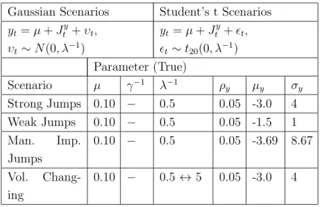
For all Gaussian simulation scenarios, one series with 1,000 observations was generated from:

yt =µ+Jty+υt, υt∼N(0, λ−1), (3.1)

same for all scenarios. Table 3.2 shows a summary of their values and simulated scenarios.

Jump componentsξy_andNy_{were generated from aN(µ}

y, σ2y) andBernoulli(ρy)

respectively. In each scenario, different values for µy and σy2 were chosen, but ρy

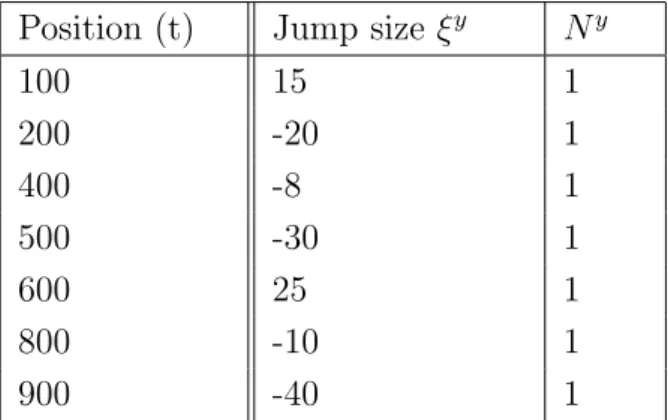
was the same. In the scenario of manually imputed jumps, together with this structure, jumps were manually imputed according to Table 3.1.

Position (t) Jump size ξy _Ny

100 15 1

200 -20 1

400 -8 1

500 -30 1

600 25 1

800 -10 1

900 -40 1

Table 3.1: Manually imputed jumps

For Student’s-t scenarios, 1,000 observations were generated from:

yt =µ+J y

t +ǫt, ǫt∼t20(0, λ−1) (3.2)

Gaussian Scenarios Student’s t Scenarios

yt =µ+Jty+υt, yt=µ+Jty+ǫt,

υt ∼N(0, λ−1) ǫt∼t20(0, λ−1) Parameter (True)

Scenario µ γ−1 _λ−1 _ρ

y µy σy

Strong Jumps 0.10 − 0.5 0.05 -3.0 4

Weak Jumps 0.10 − 0.5 0.05 -1.5 1

Man. Imp. Jumps

0.10 − 0.5 0.05 -3.69 8.67

Vol. Chang-ing

0.10 − 0.5 ↔ 5 0.05 -3.0 4

Table 3.2: Summary of Simulation Scenarios

3.2

Results and comments

Simulation results for each scenario are discussed in this section.

For model hyperparameters, the discount factorω was fixed as 0.9,αandν

vary according do simulation scenario. A G(ν

2,

ν

2) prior distribution was specified forγtin order to obtain the Student’stν-errors for the observation and system

dis-turbances. In order to keep the model comparable to Erakeret al. (2003) [9],θ =µ

component was set to be fixed over time, so that σµ2 = 0. For the mean

compo-nents,µandµy, N(0,100) priors were specified and forσ2y a InverseGamma(0.1,0.1)

prior. Also, a0 = 0.1 andb0 = 0.1, as suggested in West et al.(1987,p. 333), cited by Gamerman et al. (2013) [10]. A Beta(2,40) prior distribution was specified to

ρy, as in Eraker et al. (2003) [9].

Machine used was an Intel Core i5 - 2310 CPU at 2.90 Ghz, 4 GB RAM, and 64 bit Windows Seven operating system.

3.2.1

Simulations for the Gaussian approach

Three simulation scenarios were made using Normal distribution. The first has strong jumps, the second has weak jumps and the third includes manually imputed jumps.

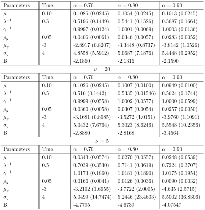
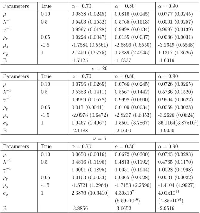
Tables 3.3, 3.4 and 3.5 show true and estimated values for each scenario. Point estimates are the posterior mean and, inside brackets, are the standard de-viation of posterior distribution. For each of three scenarios, the model parameter

ν was set as 100, 20 or 5, so that smaller values give more flexibility to the model to capture heavy tails. The threshold α was set as 0.70, 0.80 or 0.90, and gives the probability cut-point to an observation to be considered a jump.

For data generated from a Normal distribution, results suggests that the best option is to give low flexibility to the model through ν parameter. As ν

decreases, γ−1 _{component distances itself from 1, value that would indicate that} the model assumes a normal distribution for innovations. Giving flexibility to the model through ν can also influence the jump components estimates, since some jumps can be identified by the model as a mere heavy tail, thus reducing the number of jumps identified by the model, resulting in lower jump probability,

ρy, and higher jump means and standard deviation, µy and σy , since they are

ν = 100

Parameters True α= 0.70 α= 0.80 α= 0.90

µ 0.10 0.1085 (0.0245) 0.1054 (0.0245) 0.1013 (0.0245)

λ−1 0.5 0.5196 (0.1449) 0.5441 (0.1526) 0.5687 (0.1664)

γ−1 0.9997 (0.0124) 1.0001 (0.0069) 1.0003 (0.0136)

ρy 0.05 0.0406 (0.0061) 0.0346 (0.0057) 0.0283 (0.0052)

µy -3 -2.8917 (0.8207) -3.3448 (0.8737) -3.8142 (1.0526)

σy 4 4.8558 (5.5912) 5.0687 (7.1876) 5.4448 (9.2952)

B -2.1860 -2.1316 -2.1590

ν = 20

Parameters True α= 0.70 α= 0.80 α= 0.90

µ 0.10 0.1026 (0.0245) 0.1007 (0.0100) 0.0949 (0.0100)

λ−1 0.5 0.516 (0.1442) 0.5335 (0.01546) 0.5624 (0.1744)

γ−1 0.9999 (0.0558) 1.0002 (0.0577) 1.0000 (0.0599)

ρy 0.05 0.0360 (0.0058) 0.0307 (0.0054) 0.0257 (0.0050)

µy -3 -3.1681 (0.8985) -3.5272 (1.0151) -3.9760 (1.1091)

σy 4 5.0432 (7.6764) 5.3023 (8.6246) 5.5548 (10.2356)

B -2.8880 -2.8168 -3.4564

ν = 5

Parameters True α= 0.70 α= 0.80 α= 0.90

µ 0.10 0.0343 (0.0574) 0.0270 (0.0557) 0.0248 (0.0539)

λ−1 _{0.5 0.7039 (0.3530) 0.7141 (0.3619) 0.7224 (0.3707)}

γ−1 _{1.0173 (0.1860) 1.0181 (0.1890) 1.0175 (0.1954)}

ρy 0.05 0.0166 (0.0041) 0.0126 (0.0036) 0.0090 (0.0032)

µy -3 -3.2192 (1.6955) -3.7722 (2.0005) -4.635 (2.5715)

σy 4 5.0499 (14.7474) 5.2446 (23.4603) 5.5002 (36.8306)

B -4.7795 -4.6739 -4.07547

ν = 100

Parameters True α= 0.70 α= 0.80 α= 0.90

µ 0.10 0.0838 (0.0245) 0.0816 (0.0245) 0.0777 (0.0245)

λ−1 0.5 0.5463 (0.1552) 0.5765 (0.1513) 0.6001 (0.0257)

γ−1 0.9997 (0.0128) 0.9998 (0.0134) 0.9997 (0.0139)

ρy 0.05 0.0224 (0.0047) 0.0135 (0.0037) 0.0086 (0.0031)

µy -1.5 -1.7584 (0.5561) -2.6896 (0.6550) -3.2649 (0.5548)

σy 1 2.1459 (1.9775) 1.5889 (2.4945) 1.1317 (1.8626)

B -1.7125 -1.6837 -1.6319

ν = 20

Parameters True α= 0.70 α= 0.80 α= 0.90

µ 0.10 0.0796 (0.0265) 0.0766 (0.0245) 0.0726 (0.0265)

λ−1 0.5 0.5383 (0.1411) 0.5567 (0.1442) 0.5736 (0.1520)

γ−1 0.9999 (0.0578) 0.9998 (0.0600) 0.9994 (0.0622)

ρy 0.05 0.017 (0.0041) 0.0109 (0.0034) 0.0068 (0.0028)

µy -1.5 -2.0978 (0.6472) -2.8237 (0.6353) -3.2626 (0.0624)

σy 1 1.9467 (2.4967) 1.5501 (3.7867) 36.1164(3.87x104)

B -2.1188 -2.0660 -1.9050

ν = 5

Parameters True α= 0.70 α= 0.80 α= 0.90

µ 0.10 0.0650 (0.0316) 0.0672 (0.0300) 0.0743 (0.0283)

λ−1 _{0.5 0.4816 (0.1196) 0.4813 (0.1192) 0.4765 (0.1170)}

γ−1 _{1.0061 (0.1895) 1.0051 (0.1944) 1.0028 (0.1998)}

ρy 0.05 0.0103 (0.0033) 0.0065 (0.0028) 0.0031 (0.0022)

µy -1.5 -1.5721 (1.2964) -1.7153 (2.2590) -1.4104 (4.9927)

σy 1 2.3876 (10.6410) 4.30x107

(5.59x1016₎

4.01x1011 (4.85x1024₎

B -3.8856 -3.6652 -2.9516

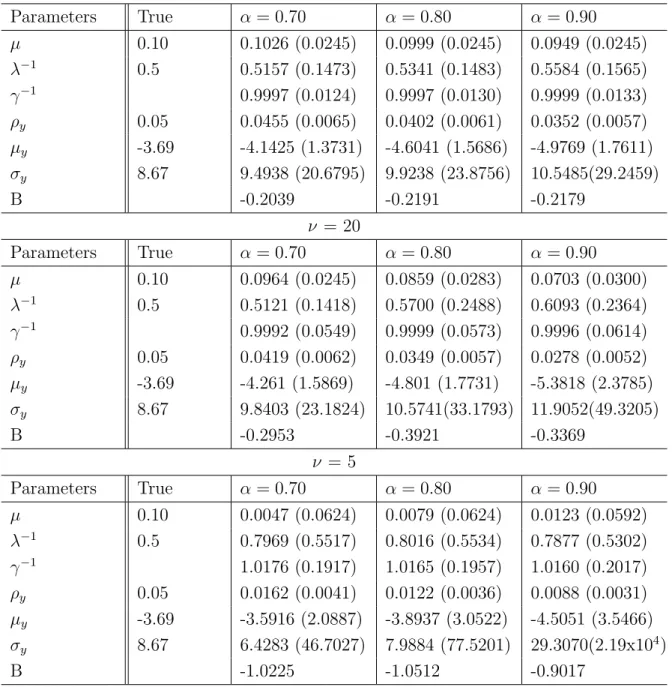
ν = 100

Parameters True α= 0.70 α= 0.80 α= 0.90

µ 0.10 0.1026 (0.0245) 0.0999 (0.0245) 0.0949 (0.0245)

λ−1 0.5 0.5157 (0.1473) 0.5341 (0.1483) 0.5584 (0.1565)

γ−1 0.9997 (0.0124) 0.9997 (0.0130) 0.9999 (0.0133)

ρy 0.05 0.0455 (0.0065) 0.0402 (0.0061) 0.0352 (0.0057)

µy -3.69 -4.1425 (1.3731) -4.6041 (1.5686) -4.9769 (1.7611)

σy 8.67 9.4938 (20.6795) 9.9238 (23.8756) 10.5485(29.2459)

B -0.2039 -0.2191 -0.2179

ν = 20

Parameters True α= 0.70 α= 0.80 α= 0.90

µ 0.10 0.0964 (0.0245) 0.0859 (0.0283) 0.0703 (0.0300)

λ−1 0.5 0.5121 (0.1418) 0.5700 (0.2488) 0.6093 (0.2364)

γ−1 0.9992 (0.0549) 0.9999 (0.0573) 0.9996 (0.0614)

ρy 0.05 0.0419 (0.0062) 0.0349 (0.0057) 0.0278 (0.0052)

µy -3.69 -4.261 (1.5869) -4.801 (1.7731) -5.3818 (2.3785)

σy 8.67 9.8403 (23.1824) 10.5741(33.1793) 11.9052(49.3205)

B -0.2953 -0.3921 -0.3369

ν = 5

Parameters True α= 0.70 α= 0.80 α= 0.90

µ 0.10 0.0047 (0.0624) 0.0079 (0.0624) 0.0123 (0.0592)

λ−1 _{0.5 0.7969 (0.5517) 0.8016 (0.5534) 0.7877 (0.5302)}

γ−1 _{1.0176 (0.1917) 1.0165 (0.1957) 1.0160 (0.2017)}

ρy 0.05 0.0162 (0.0041) 0.0122 (0.0036) 0.0088 (0.0031)

µy -3.69 -3.5916 (2.0887) -3.8937 (3.0522) -4.5051 (3.5466)

σy 8.67 6.4283 (46.7027) 7.9884 (77.5201) 29.3070(2.19x104)

B -1.0225 -1.0512 -0.9017

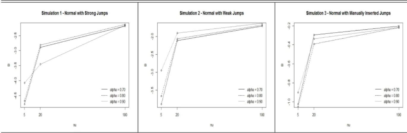
Figure 3.1: Normal Simulations - B-statistic comparison

Figure 3.1 shows a comparison between B-statistics for each simulation scenario. In all cases a higher ν gave a better model fit. On the other hand, for each case a different choice threshold α gave a better fit. Overall α = 0.7 seems to be a good choice, since its results are reasonably good for both strong and manually imputed jumps, being the worst choice only for weak jumps, where the model is known to have difficult on estimating parameters independently of parameters choice.

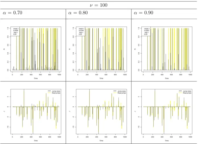
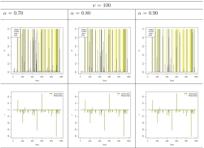
ν = 100

α = 0.70 α = 0.80 α = 0.90

Figure 3.2: Simulation 1 - Normal with Strong Jumps - Jump probabilities and sizes

For strong jumps, Figure 3.2, it is possible to see that as the threshold α

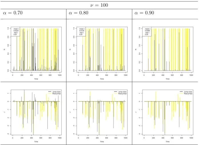
ν = 100

α = 0.70 α = 0.80 α = 0.90

Figure 3.3: Simulation 2 - Normal with Weak Jumps - Jump probabilities and sizes

For weak jumps, Figure 3.3, it is possible to see that, independently of the choice of α, the model has difficult on estimating jump probabilities and sizes. Only the biggest jumps are considered by the model, which explains the higherµy

and σy estimates seen on Table 3.4. Since the model uses the observations that

ν = 100

α = 0.70 α = 0.80 α = 0.90

Figure 3.4: Simulation 3 - Normal with Manually Imputed Jumps - Jump proba-bilities and sizes

For manually imputed jumps, Figure 3.4, results were very similar to strong jumps, again giving the lead to α = 0.70, since gives jump probability estimate closer to the true. The model was able to capture all the manually imputed jumps, no matter what was the choice of α.

3.2.2

Sudent’s t Simulations

includes manually imputed jumps.

A forth simulation was made in order to verify how volatility changes affects jump related parameters estimation. For this case, model parameters were fixed at

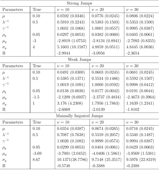
ν= 30 andα= 0.7, as suggests the previous simulation results. In this simulation, three scenarios were built: first on which true λ−1 _{assumes 0.5; second with true}

Strong Jumps

Parameters True ν= 10 ν= 20 ν = 30

µ 0.10 0.0592 (0.0346) 0.0776 (0.0245) 0.0806 (0.0224)

λ−1 _{0.5 0.5910 (0.2243) 0.5383 (0.1503) 0.5353 (0.1500)}

γ−1 _{1.0031 (0.1068) 1.0001 (0.0557) 0.9995 (0.0387)}

ρy 0.05 0.0297 (0.0053) 0.0382 (0.0060) 0.0405 (0.0061)

µy -3 -2.8919 (1.0753) -2.8134 (0.8941) -2.7093 (0.8355)

σy 4 5.1603 (10.1587) 4.8859 (6.0511) 4.8445 (6.0036)

B -2.9944 -3.0956 -2.3654

Weak Jumps

Parameters True ν= 10 ν= 20 ν = 30

µ 0.10 0.0491 (0.0300) 0.0603 (0.0245) 0.0681 (0.0245)

λ−1 0.5 0.5385 (0.1371) 0.5534 (0.1466) 0.5592 (0.1507)

γ−1 1.0019 (0.1091) 1.0000 (0.0592) 0.9998 (0.0412)

ρy 0.05 0.0138 (0.0038) 0.0177 (0.0042) 0.0191 (0.0044)

µy -1.5 -2.1209 (0.6937) -2.3737 (0.4834) -2.4673 (0.3964)

σy 1 3.176 (4.2308) 1.7956 (1.7863) 1.1639 (1.2341)

B -2.6069 -2.0139 -1.8102

Manually Imputed Jumps

Parameters True ν= 10 ν= 20 ν = 30

µ 0.10 0.0354 (0.0387) 0.0674 (0.0265) 0.0716 (0.0245)

λ−1 _{0.5 0.7087 (0.7638) 0.5559 (0.2057) 0.5340 (0.1487)}

γ−1 _{1.0026 (0.1082) 0.9999 (0.0574) 0.9994 (0.0387)}

ρy 0.05 0.0299 (0.0053) 0.0404 (0.0061) 0.0429 (0.0063)

µy -3.69 -3.7001 (2.0452) -4.0406 (1.5861) -3.9569 (1.5381)

σy 8.67 10.1371(38.7786) 9.7148 (25.3517) 9.5976 (22.8319)

B -0.5748 -0.3388 -0.2388

Table 3.6: Simulation 4 - Student’s t - 20 degrees of freedom

disrupts the capability of the model to identify jumps, it seems that a slightly higher value for ν can improve model sensibility for jumps.

Figure 3.5: B-statistics comparison for Student’s t scenario

Figure 3.5 shows the comparison between B-statistics for each scenario. For all casesν = 30 has a higher B-statistic. Curiously, for strong jumps scenario,

ν = 10 ν = 20 ν = 30

Figure 3.6: Simulation 4 - Strong Jumps - Jump probabilities and sizes

ν = 10 ν = 20 ν = 30

Figure 3.7: Simulation 4 - Weak Jumps - Jump probabilities and sizes

ν = 10 ν = 20 ν = 30

Figure 3.8: Simulation 4 - Manually Imputed Jumps - Jump probabilities and sizes

Trueλ−1 = 0.5 True λ−1 = 5 Trueλ−1 = 0.5 and 5

Figure 3.9: Simulation 5 - Influence of volatility changes

Figure 3.9 shows the effect of volatility changes on jump estimates. Con-tinuous line represents the posterior mean and the gray area indicates the 95% credibility interval. Increases on estimated volatility affect the model increasing tail weight, since in the model υt|γt ∼ N(0, γt−1λ−t1). Therefore, some outliers

affecting jump probabilities and size estimates. However, such effect was already expected, since in moments of market tensions, where risk rises above normal, ex-cess in returns are not merely isolated speculative movements, that can be capture by the jump component, but reflex of the increase in market risk. It is notable that the model was able to capture the changes in volatility over the time, which is particularly important, since the main focus is on precisely estimating changes in volatility, which represents market risk.

3.3

Simulation conclusions

Based on simulations, it is possible to conclude that the model is able to capture both jump and heavy tails structures and estimate parameters with good precision. The model has some difficulty on estimating jump size variance, since estimation is based only observations which are considered jumps by the model, leading to a value generally higher than true parameter. It is also evident that when jumps are weak, the model has trouble on recognizing them, which leads to a drop on jump probabilities estimative and increase in jump sizes variance. This problem is worsen for higher threshold α values and smaller ν values.

Simulated data suggests that, for practical applications, where there is not much time and computational resources available and real parameters are not known, using α = 0.70 and ν = 30 would bring best results overall, but such parameters can be specified in other way by model user. If there is time and computational resources available, a sensibility analysis can be made for a grid of different α and ν values, as shown on the simulations, and best model can be chosen based on B-statistics.

Chapter 4

Applying model to stock market

index data

Figure 4.1: S&P500 log return histogram Figure 4.2: iBovespa log return histogram

Mean Variance Skewness Kurtosis Min Max S&P500 0.05205 0.9978 -2.6357 63.0710 -22.8997 8.7089 iBovespa 0.0134 0.6137 -0.0931 7.3176 -5.2533 5.94038

Table 4.1: Summary Statistics

Figure 4.3: S&P500 log return series Figure 4.4: iBovespa log return series

index. Two main reasons for that are: the period being analyzed, since economy characteristics substantially changed from the decade of 80 to year 2000 and on; and also mechanisms of limiting loss that were recently implemented, in which assets trade are suspended in case of a big daily loss or gain. Due to such mecha-nisms, speculative movements are limited, avoiding big losses as the one observed in S&P500 of 22.89% in one day. Due to that, it is expected that jumps will play a much greater role on american index than brazilian.

For applying on stock market index data, based on simulations conclusion that suggest ν = 30, a G(15,15) prior distribution was specified forγt in order to

obtain the Student’s t30-errors for the observation and system disturbances. The threshold, based on simulations conclusion, was fixed at α= 0.7 and the discount factor ω fixed at 0.9. All other priors and the MCMC parameters were specified in the same way it was for simulation, in section 3.2. MCMC results are shown on Appendix D.

4.1

S&P 500

Table 4.2 provides parameter posterior means and standard deviation for the proposed model. λ−1 _{value represents mean and standard deviation for the set} of λ−t1 means. Analogously, γ refers to the set ofγ.

Parameter Estimated value

µ 0.0658 (0.01066)

λ−1 _{2.3529 (1.5823)}

γ 0.9997 (0.0409)

ρy 0.0149 (0.0022)

µy -0.3567 (0.3895)

σy 2.6999 (0.2906)

B -1.8454

Figure 4.5 provides jump sizes and probabilities for each observation. As observed on simulations, part of the excess in returns are absorbed by the dis-tribution tail or in the form of an increase in variance, which would mean an increase on the risk measure. Before periods of higher volatility, it is possible to observe an increase in jump sizes and probabilities, when compared to periods with lower volatility, thus evidencing that such periods are preceded by speculative movements, captured in the model by jumps.

Figure 4.6 provides spot volatility estimates over the whole period, Jan/1980 to Dec/1999, and over two specific periods, 1987 to 1989, when took place the Black Monday, on Oct/1987, and 1997 to 1999, when Asian and Russian financial cri-sis shaken the stock market. Continuous line represents the posterior mean and the gray area indicates the 95% credibility interval for spot volatility. Although measure differs, since a different distribution specification was made, volatility be-havior is consistent with Eraker et al. (2003) [9] findings, with peaks occurring at the same time.

Figure 4.7 provides posterior mean for mixture component γ. As it gets farer from 1, it indicates increasing activity on capturing heavy tails in returns. A distinguishable point is seen on Oct/1987, when Black Monday occurred. The model consider this point as a heavy tail event, thus reducing jump size on that point and increasing volatility measure. Variance, Figure 4.8, defined as γt−1λ−t1

Figure 4.6: Estimated volatility for the S&P500 index. Continuous line represents the posterior mean. The grey area indicates the 95% credibility intervals.

Figure 4.7: Mixture component, γt Figure 4.8: Variance,γt−1λ

−1

4.2

iBovespa

Table 4.3 provides parameter posterior means and standard deviation for the proposed model. λ−1 _{value represents mean and standard deviation for the set} of λ−t1 means. Analogously, γ refers to the set ofγ.

Parameter Estimated value

µ 0.0300 (0.0107)

λ−1 _{0.5655 (0.6741)}

γ 0.9997 (0.0389)

ρy 0.0090 (0.0021)

µy -0.3025 (0.4947)

σy 1.9987 (0.3357)

B -1.6640

Table 4.3: Parameter estimates for iBovespa index data

Figure 4.9 provides jump sizes and probabilities for each observation. Since iBovespa returns on this period is more stable when compared to S&P 500 index on 1987 to 1999 period, jump sizes and probabilities are smaller than what is observed in American index. Since log return magnitudes are smaller than S&P’s, model heavy tails tend to accomodate more observations, which also reduces jump probability and size estimates. In iBovespa index, increase on jumps probabilities and sizes can also be observed days before increases on volatility, so that the presence of higher jumps can indicate near future increases on market risk.

Figure 4.11 provides posterior mean for mixture component γt. As it gets

farer from 1, it indicates activity on capturing heavy tails in returns. It’s possible to see that this component is persistently capturing heavy tails, which can explain the absence of stronger jumps for this market. Variance (Figure 4.12) defined as

Figure 4.10: Estimated volatility for the iBovespa index. Continuous line repre-sents the posterior mean. The grey area indicates the 95% credibility intervals.

Figure 4.11: Mixture component, γt Figure 4.12: Variance, γt−1λ

−1

4.3

Experimental conclusions

The NGSVJ model was able to capture speculative movements in the mar-ket through the jump components and detect periods with increased marmar-ket risk through the volatility component. Results obtained by applying the model to S&P 500 return series are consistent with Eraker et al. (2003) [9] findings, since volatility peaks occur at same times. Historical events of known volatility effects on financial markets, such as Black Monday and Asian/Russian Financial Crisis, for S&P index, and Subprime crisis and Presidential Elections, for iBovespa index, can be detected by the model precisely.

Results also suggest that the model can adapt to data despite the charac-teristics of the market being analysed. Jumps play a greater role on markets with bigger discrepancy between returns, like in S&P index, where log returns ampli-tude is around 31 points, three times bigger than iBovespa’s log returns amplited of just around 11 points. On iBovespa index, less jumps are detected and some of excess returns are absorbed by distribution tail.

Chapter 5

A proposal for weak jumps

scenario

This chapter presents an alternative method for jump detection and simu-lations on using such method.

5.1

Jump Detection Algorithm: a Non-Parametric

Approach

and Maykland (2008) [14]. If the length for analysis is 1, the algorithm for the process is given by the following chart.

Figure 5.1: Block average jump detection flowchart. Source: Riley(2008).

In other words, if the observation yt+1 is out of the interval yt ± Z ×

p

γt−1λ−1, whereZ is a threshold selected according to the area of a Normal curve

corresponding to a tail probability1_{, it is considered a jump at time t+ 1.}

The jump probabilities can be easily calculated by getting the average value ofJt. The average in this case would be the number of times there was considered

a jump at time t divided by the number of iterations taken, which would be a number inside [0,1].

1_{Based on a N(0,1) test on which Z refers to the value in which probability of occurrence is}

5.2

Simulations

For the non-parametric approach, the simulation data used was the same as Simulation 4 - Student’s t distribution with 20 degrees of freedom and weak jumps. For a Z selected so that the cut-point is 95% and 99% of a Normal curve, three different values for ν were tested: 10, 20 and 30.

Figure 5.2: B-statistics comparison for Student’s t scenario - Non Parametric Approach

Weak Jumps - NGSVJ

Parameters True ν= 10 ν= 20 ν = 30

µ 0.10 0.0491 (0.0300) 0.0603 (0.0245) 0.0681 (0.0245)

λ−1 _{0.5 0.5385 (0.1371) 0.5534 (0.1466) 0.5592 (0.1507)}

γ−1 _{1.0019 (0.1091) 1.0000 (0.0592) 0.9998 (0.0412)}

ρy 0.05 0.0138 (0.0038) 0.0177 (0.0042) 0.0191 (0.0044)

µy -1.5 -2.1209 (0.6937) -2.3737 (0.4834) -2.4673 (0.3964)

σy 1 3.176 (4.2308) 1.7956 (1.7863) 1.1639 (1.2341)

B -2.6069 -2.0139 -1.8102

Weak Jumps - Non Parametric Approach - cut 99%

Parameters True ν= 10 ν= 20 ν = 30

µ 0.10 0.0711 (0.0391) 0.0692 (0.0331) 0.0706 (0.0349)

λ−1 0.5 0.4866 (0.1087) 0.5100 (0.1149) 0.5163 (0.1122)

γ−1 1.0019 (0.0979) 0.9986 (0.0555) 0.9993 (0.0384)

ρy 0.05 0.0483 (0.0066) 0.0453 (0.0064) 0.0453 (0.0064)

µy -1.5 -1.9811 (1.7849) -1.9665 (1.3807) -1.8711 (1.2589)

σy 1 2584.51(77880.84) 2.7826(6.0222) 2.4737 (1.1679)

B -5.6193 -3.3669 -2.8792

Weak Jumps - Non Parametric Approach - cut 95%

Parameters True ν= 10 ν= 20 ν = 30

µ 0.10 0.086 (0.0363) 0.0814 (0.0301) 0.0817 (0.0278)

λ−1 _{0.5 0.3983 (0.0811) 0.3996 (0.0794) 0.4022 (0.0791)}

γ−1 _{0.9986 (0.0873) 0.9963 (0.0489) 0.9966 (0.0342)}

ρy 0.05 0.1168 (0.0098) 0.1113 (0.0096) 0.1145 (0.0098)

µy -1.5 -1.0547 (1.1567) -0.9757 (0.7974) -0.9108 (0.6494)

σy 1 1.9908 (0.645) 2.0355 (0.5762) 1.9908 (0.645)

B -∞ -5.9567 -4.0273

Table 5.1: Simulation 6 - Non-Parametric Approach - Student’s t - 20 degrees of freedom

num-ber of outliers stays more or less the same. For cut-point = 99% and ν = 30, non-parametric approach shows point estimates slightly closer to real values than other models in general. However, B-statistics indicates that model fit is worse than NGSVJ parametric approach. Figure 5.3 gives a glue of the reason why this happens: even though point estimate matches with real value, model is not able to capture precisely jump times, underestimating probabilities for real jump times and detecting jumps where there are not.

Using cut-point = 95%, the model over-estimates jump probabilities. This leads to worse B-satistics when compared to other models.

NGSVJ -ν = 30 NP - 99% NP - 95%

Figure 5.3: Simulation 6 - Weak Jumps - Non-Parametric Approach

5.2.1

Simulation conclusions

Chapter 6

Discussion about the NGSVJ

model

There are a lot of works on stochastic volatility models for univariate fi-nancial time series. This work used as base for comparison the models presented by Eraker et. al. (2003) [9], but there are also developments on SV models, as the proposed by Warty et al (2014) [26], using variance-gamma jumps, and Nakajima and Omori (2007) [18], including in the model the leverage effect together with heavy tails and correlated jumps.

Since a lot has been already discussed on these previous works, one might ask what is the gain on continue developing methods to model volatility for uni-variate financial time series. This chapter focus on discussing the key points that justify the importance of NGSVJ model as an alternative to the classic SV model and its variations.

6.1

NGSVJ model advantages

and the structure of the DLM model, on which it is based, that grants an automatic sampling process for parameters.

Using Gibbs Sampler to obtain a sample from conditional posterior distri-butions is computationally cheaper than recurring to Metropolis based algorithms. Since Metropolis is an accept-reject algorithm, it can take several steps until a full sample is obtained in order to make statistical inference, unless a very good pro-posal distribution is given to the algorithm. On using Gibbs Sampler, only one step is needed in order to obtain the same sample. This is specially relevant when dealing with high dimensional data, such as market daily returns from several years.

Due to this computational simplicity, NGSVJ model can be run on an ordinary home computer and give reliable results for analysis in some hours, even for long iteration chains, such as 100,000 observations. The practical consequence of such advantage is that the model can be run after market closes and results will be available before market opens on the next day. Also, it can potentially bring cost reductions and be available for any market player, since there is no need for advanced hardware configuration in order to the computer to run the model.

As the model is build over the Dynamic Linear Model with scale mixtures proposed by Gamermanet al.(2013) [10], it takes advantage of the sampling process mentioned on Chapter 2.4.1. Theorems 1 and 2 cited by Gamermanet al. (2013) [10] can be applied so that an exact sample of Volatility parameterλ−_t1is obtained. The two main advantages that comes from this process are: there is no need to make approximations in order to estimate volatility, and it is a faster method, since all parameters are sampled at once.

6.2

Comparison to other models

Since SV models presented by Erakeret al. (2003) [9] have a different struc-ture from the proposed model, comparison between models is not straightforward. Comparison can be made between parameters that exist on both NGSVJ and SV models with the same roles on both models, that is, equilibrium return and jump related parameters. Table 6.1 compares posterior mean of common parameters estimates between the proposed model and the stochastic volatility with jumps on returns (SVJ), with independently arriving jumps on returns and volatility (SVIJ) and contemporaneous arriving jumps (SVCJ), omitting the ones that are exclusive for each model, for S&P 500 returns.

NGSVJ SVJ SVCJ SVIJ

µ 0.0658 (0.01066) 0.0496 (0.0109) 0.0554 (0.0112) 0.0506 (0.0111)

ρy 0.0149 (0.0022) 0.0060 (0.0021) 0.0066 (0.0020) 0.0046 (0.0020)

µy -0.3567 (0.3895) -2.5862 (1.3034) -1.7533 (1.5566) -3.0851 (3.2485)

σy 2.6999 (0.2906) 4.0720 (1.7210) 2.8864 (0.5679) 2.9890 (0.7486)

Table 6.1: Comparison between NGSVJ model and SVJ models in Eraker et. al (2003) [9] for S&P 500 returns

NGSVJ model captures more jump points than Eraker et al. (2003) [9] SV models. This leads to a smaller estimative for µy, since more points are captured

Chapter 7

Conclusion

The proposed model has a much more simple structure to deal with the inclusion of heavy tails and jumps than the other methods commonly used. The possibility of using only Gibbs Sampling method to sample from the posterior distributions, together with the block sampling structure, give efficiency and speed to the model, which is crucial in day-to-day operations.

The inclusion of jumps in the model reduces substantially the volatility estimate. This would have several impacts on risk analysis, since less volatility indicates less risk, in other words, knowing that some event was a jump, or tail event, and not a recurrent market event would mean that such asset is still a safe bet. Usually an increase of jump frequency is observed near the occurrences of market anomalies, such as Black Monday and the Asian and Russian financial crisis, in S&P 500, and 2008 crisis and Brazilian presidential elections, in iBovespa, which may indicate that it can also be used for predicting near future increases on market risk.

The easiness to include mixture variables in the model is another advantage. By doing that, there are no simplifications of reality by assuming Gaussian distri-bution, since it is well documented on the literature that financial asset returns data have heavy tailed distribution.

first is due to dealing with high dimensional data, to keep up speed and save memory in the computer, optimizations must be done in the code in order to be able to run it. Such optimizations include: block sampling, squeezing the number of variables declared and the dimensionality of such variables, creating a burn-lags routine such that it only saves values that are in fact relevant; the second is on estimating jumps when jump sizes are small, since the model struggles to detect jumps that are inside distribution tail, which is worsen by using a heavy tailed distribution.

The attempt of using a non-parametric method, based on a normal curve tail analysis, such as proposed by Riley (2008) [21], for detecting jumps in a weak jumps scenario was not effective, since there is a lot of miss-classification using such method, which causes more harm than good to the model.

For day-to-day operations, the automatic model is effective and can be used in order to estimate market volatility, which can be used for options pricing, VaR calculations, measuring risk, etc. Its lower computational cost compared to Metropolis-based algorithms make it accessible to firms and investors who does not have access to high technology computers - common personal computers are able to run the model and bring reliable results in some hours. Using an Intel Core i5 -2310 CPU at 2.90 Ghz, 4 GB RAM, and 64 bit Windows Seven operating system, it took approximately 7 hours to get results from S&P 500 index and 5 hours and a half to get results from iBovespa index.

Bibliography

[1] Abanto-Valle, C. Lachos, V. and Dey, D. (2015). Bayesian Estimation of a Skew-t Stochastic Volatility Model. Methodology and Computing in Applied Probability, 17:721–738.

[2] Bollerslev, T. Gibson, M. and Zhou, H. (2010). Dynamic estimation of volatil-ity risk premia and investor risk aversion from option-implied and realized volatilities. Journal of Econometrics, 160:235–245.

[3] Brooks, C. and Prokopczuk, M. (2011). The Dynamics of Commodity Prices. ICMA Centre Discussion Papers in Finance, DP2011-09.

[4] Chib, S. Nardari, F. and Shephard, N. (2002). Markov chain Monte Carlo methods for stochastic volatility models. Journal of Econometrics, 108:281– 316.

[5] Demarqui, F.N.(2010). ”Uma classe mais flex´ıvel de modelos semiparamtricos para dados de sobrevivncia”. UFMG. Doctoral Thesis. Belo Horizonte.URL: http://est.ufmg.br/portal/arquivos/doutorado/teses/TeseFabioDemarquiFinal.pdf

[6] Doornik, J.A.(2008). Ox Edit 5.10 [Computer Software]. Retrieved from http://www.doornik.com/ox/.

[7] Dowd, K.(2002). Measuring market risk. Wiley, England.

[8] Duffie, D. and Pan, J. (1997). An Overview of Value at Risk. The Journal of Derivatives, 3:7–49.

[10] Gamerman, D. Santos, T. and Franco, G. (2013). A Non-Gaussian Family of State-Space Models With Exact Marginal Likelihood. Journal of Time Series Analysis, 34:625–645.

[11] Hendricks, D. (1995). Evaluation of Value-at-Risk Models Using Historical Data. Working paper, Federal Reserve Bank of New York.

[12] Ibrahim, J. G. Chen, M.H. and Sinha, D. (2001). Bayesian survival analysis. Springer-Verlag, New York.

[13] Kungl. Vetenskaps-Akademien. (2013). Understanding Asset Prices Scientific Background on the Sveriges Riksbank Prize in Economic Sciences in Memory of Alfred Nobel 2013, 1–55.

[14] Lee, S. and Maykland, P. (2008). Jumps in Financial Markets: A New Nonparametric Test and Jump Dynamics. The Review of Financial Studies, 21:2535–2563.

[15] Li, H. Wells M. and Yu, C. (2008). A Bayesian Analysis of Return Dynamics with Levy Jumps. Review of Financial Studies, 21:2345–2378.

[16] Merener, N. (2015). Concentrated Production and Conditional Heavy Tails in Commodity Returns. The Journal of Futures Markets, XX:1–20.

[17] Nakajima, J. and Omori, Y. (2007). Leverage, Heavy-Tails and Correlated Jumps in Stochastic Volatility Models. CARF Working Paper, CARF-F-107.

[18] Omori, Y. Chib, S. Shephard, N. and Nakajima, J. (2007). Stochastic volatil-ity with leverage: Fast and efficient likelihood inference Journal of Econo-metrics, 140: 425–449.

[19] Prado, R. and West, M. (2010). Time Series Modeling, Computing and In-ference. CRC Press, Boca Raton.

[20] Raftery, A.E. and Lewis, S.M. (1992). How many iterations in the Gibbs sampler?. Bayesian Statistics, 4:765–776.

[22] Schwartz, E. and Smith, J. (2000). Short-Term Variations and Long-Term Dynamics in Commodity Prices. Management Science, 46:893–911.

[23] The R foundation for Statistical Computing.(2015). R version 3.2.1 [Computer Software]. Retrieved from http://www.r-project.org/.

[24] Todorov, V. (2010). Variance Risk-Premium Dynamics: The Role of Jumps. Review of Financial Studies, 23:345–383.

[25] Triantafyllopoulos, K. (2008). Multivariate stochastic volatility with Bayesian dynamic linear models. Journal of Statistical Planning and Inference, 138:1021–1037.

[26] Warty, S. Lopes, H. and Polson, N. (2014). Sequential bayesian learning for stochastic volatility with variance-gamma jumps in returns. Insper Working Paper, WPE:340/2014.

[27] West, M. and Harrison, J. (1997). Bayesian Forecasting and Dynamic Models. Springer, New York.

Appendix A

Full Conditional Posterior

Distributions for NGSV Model

This appendix presents the conditional posterior distributions for the vari-ables NGSVJ model. For simplifying notation, let Φ = (θt, Jty, γt, δt, λt, σu2) be all

other model variables, excluding the one which conditional posterior distribution is being calculated.

A.1

Conditional Posterior Distribution for

γ

p(γt) ∼ Gamma(

ν

2,

ν

2)

p(γt|yt,Φ[−γ]) ∝ (γt)

ν

2−1e−γt

ν

2

1

γt−1λ−t1

12

exp

−(Yt−Ftθt−Jt) 2

2γt−1λ−t1

p(γt|yt,Φ[−γ]) ∝ (γt)

ν

2+ 1 2−1exp

−γt

ν

2 +λt

(Yt−Ftθt−Jt)2

2

p(γt|yt,Φ[−γ]) ∼ Gamma

ν 2 + 1 2, ν

2 +λt

(Yt−Ftθt−Jt)2

2

A.2

Conditional Posterior Distribution for

δ

p(δt) ∼ Gamma(

ν

2,

ν

2)

p(δt|yt,Φ[−δ]) ∝ (δt)

ν

2−1e−δt

ν

2|δ−1

t (σµ2)|

−1

2 exp −

(θt−θt−1)(δ−t1(σµ2))−1(θt−θt−1)

2

!

p(δt|yt,Φ[−δ]) ∝ (δt)

ν

2+ 1 2−1exp

−δt

ν

2 +

(θt−θt−1)(σµ2)−1(θt−θt−1) 2

p(δt|yt,Φ[−δ]) ∼ Gamma

ν 2 + 1 2, ν 2 +

(θt−θt−1)(σµ2)−1(θt−θt−1) 2

.

A.3

Conditional Posterior Distribution for

σ

p(σ_µ2) ∼ InverseGamma(a0, b0)

p(σ_µ2|yt,Φ[−σ2

µ]) ∝

1

σ2

µ

a0+1

e− b0 σ2 µ n Y i=2 1

δ_i−1σ2

µ

!12

exp −

n

X

i=2

(θi−θi−1)2

2δ−_i 1σ2

µ

!

p(σ_µ2|yt,Φ[−σ2

µ]) ∝

1

σ2

µ

a0+1

e− b0 σ2 µ 1 σ2 µ n2

exp − 1 2σ2

µ n

X

i=2

δi(θi−θi−1)2

!

p(σ_µ2|yt,Φ[−σ2

µ]) ∝ (σ 2

µ)

−(a0+n₂+1) exp

− 1

σ2

µ

b0+

Pt

i=2δi(θi−θi−1)2

2

p(σ_µ2|yt,Φ[−σ2

µ]) ∼ InverseGamma

a0+

n

2, b0 +

Pt

i=2δi(θi−θi−1)2 2

Appendix B

Full Conditional Posterior

Distributions for Jump

Components

This appendix presents the conditional posterior distributions for the jump components: µy,σ2y,ξ

y t+1N

y

t+1andρ. For simplifying notation, let Φ = (θt, Jty, γt, δt, λt, σ2u)