AGFORWARD (Grant Agreement N° 613520) is co-funded by the European Commission, Directorate General for Research & Innovation, within the 7th Framework Programme of RTD. The views and opinions expressed in this report are purely those of the writers and may not in any circumstances be regarded as stating an official position of the European Commission
Modelling the economics of agroforestry
at field- and farm-scale
Project name AGFORWARD (613520)
Work-package 6: Field- and farm-scale evaluation of innovations
Deliverable Deliverable 6.18: Modelling the economics of agroforestry at field- and farm-scale
Date of report 31 August 2017 (updated 13 October 2017)
Authors Silvestre García de Jalón, Anil Graves, Joao Palma, Josep Crous-Duran, Michail Giannitsopoulos, Paul J Burgess
Contact a.graves@cranfield.ac.uk s.garciadejalon@gmail.com
Reviewed Paul Burgess (18 August 2017)
Contents
1 Context and objectives ... 2
2 Methodological framework ... 2
3 The Farm-SAFE model ... 3
4 Modelling and valuing the environmental impacts of arable, forestry and agroforestry systems: a case study ... 26
5 The Forage-SAFE model ... 41
6 Up-scaling: from farm to regional scale ... 48
7 Conclusions ... 61
8 Acknowledgements ... 62
9 References ... 62
1 Context and objectives
The AGFORWARD research project (January 2014-December 2017), funded by the European Commission, is promoting agroforestry practices in Europe that will advance sustainable rural development. The project has four objectives:
1. to understand the context and extent of agroforestry in Europe,
2. to identify, develop and field-test innovations (through participatory research) to improve the benefits and viability of agroforestry systems in Europe,
3. to evaluate innovative agroforestry designs and practices at a field-, farm- and landscape scale, and
4. to promote the wider adoption of appropriate agroforestry systems in Europe through policy development and dissemination.
The third objective of the project is addressed in work-package 6 which focused on the field- and farm-scale evaluation of innovations, and work-package 7 which focused on the landscape evaluation.
Within work-package 6 deliverables 6.16 and 6.17 focus on the biophysical evaluation of agroforestry systems at the field- and farm-scale. This report (Deliverable 6.18) assesses the economics of agroforestry systems at field- and farm-scales and compares them with alternative land uses such as arable cropping, pasture and forestry. More specifically this report evaluates the financial profitability (from a farmer perspective) and the economic benefits (from a societal perspective). The report also explores how farm-scale modelling results can be up-scaled at the regional level.
2 Methodological framework
This study used biophysical and economic models to assess the economics of agroforestry systems and to compare them with arable, pasture and forestry systems. The biophysical model used in this report was the Yield-SAFE model (van der Werf et al. 2007; Palma et al. 2017). The Yield-SAFE model is a parameter-sparse, process-based dynamic model for predicting resource capture, growth, and production in agroforestry systems that has been frequently used by various research organizations in recent years. It works on a daily time-step for a specified rotation of the trees that may last a given number of years.
Numerous improvements to two models have been undertaken to assess the economics of agroforestry, arable, pasture and forestry systems:
The Farm-SAFE model: this is a Microsoft Excel-based spreadsheet model (Graves et al. 2007; 2011) that evaluates the financial and economic costs and benefits of arable, forestry, silvoarable, and silvopastoral systems. It works at an annual time-step and assesses the economics for a whole rotation of the trees (maximum rotation length = 60 years). The model was developed during the SAFE project to initially assess the financial profitability of silvoarable systems (Dupraz et al. 2005).
The Forage-SAFE model: this is a Microsoft Excel-based spreadsheet model (García de Jalón et al. 2017) that evaluates the management and economics of wood pasture systems. It works at a daily time-step and assesses the economics for one year in a steady state scenario. This is a new model that has been developed during the AGFORWARD project (Burgess et al. 2015).
Modelling the economics of agroforestry www.agforward.eu This report assesses the profitability of agroforestry systems in multiple case studies across Europe. It also presents the improvements carried out in the Farm-SAFE and Forage-SAFE models during the AGFORWARD project. Within this report two peer-reviewed papers have been produced to show the improvements made in the Farm-SAFE model and to describe the Forage-SAFE model.
The remainder of the report is separated into six main sections. The first section briefly describes the Farm-SAFE model, shows the improvements developed in the AGFORWARD project and presents results for various agroforestry, arable and forestry systems in Europe. This is followed by a peer-reviewed paper that uses the Farm-SAFE model to predict the environmental impact of agroforestry relative agriculture and forestry. The next section introduces the Forage-SAFE model which has been produced within the framework of work-package 6. This section describes in detail how the model works as well as its applicability. It assesses the economic impact of managerial decisions on the profitability of wood pastures (e.g. tree cover density and carrying capacity). This is followed by a peer-reviewed paper that has been produced within this deliverable has been incorporated. The next section presents a methodology developed to up-scale farm-level results to the regional level. The region of Britany (France) was used as a case study to show the applicability of the approach. The last section describes the main conclusions of this report.
3 The Farm-SAFE model
Farm-SAFE is a Microsoft Excel-based spreadsheet model (Graves et al. 2007; 2011) that evaluates the financial and economic costs and benefits of arable, forestry and silvoarable systems. Farm-SAFE was developed within the framework of the SAFE project which aimed to provide guidelines on the viability of silvoarable systems in Europe and the extrapolation of plot-scale results to individual farms (Dupraz et al. 2005). The model integrates biophysical outputs of Yield-SAFE with financial/economic data for analyses and environmental outputs at farm-scale. The main objectives of Farm-SAFE were described in Graves et al. (2011). These were:
To use a common conceptual framework of farm economics including net margins To account for the effect of time on the value of money by discounting
To compare the profitability of the systems. Discounted future benefits and costs of each system should be aggregated and a net present value, infinite net present value, and equivalent annual value calculated.
To determine the feasibility of the systems. In particular, the effect of introducing the new agroforestry system on existing farm could be studied in terms of annual labour requirements, cash flow requirements and net benefit effects.
To examine the sensitivity of each system to changes in input values
Within the AGFORWARD project (Burgess et al. 2015), the application and objectives of the Farm-SAFE model has been extended, so that in addition to assessing the financial performance of arable, forestry and agroforestry systems, it can quantify and compare the environmental externalities. In combination with the Yield-SAFE model, Farm-SAFE can now evaluate the provision of ecosystem services. For instance, in addition to calculating the economic value of “provisioning” services (i.e. yields) of trees, crops, and livestock, which are frequently obtained from Yield-SAFE, the economic value of the “supporting” (e.g. soil nutrients) and “regulating” services (e.g. carbon capture, water quality, GHG emissions) of agroforestry systems can also were evaluated by using a Life Cycle Assessment that has been implemented within Farm-SAFE. The cultural services (e.g. aesthetic
pleasure, recreation potential) of agroforestry systems could also be evaluated within Farm-SAFE by using a range of social, and environmental economic research methods to identify, quantify, and rank social perceptions and preferences for agroforestry products and systems. However, on the whole, it has been difficult to obtain economic values for cultural services.
The development of an ecosystem services approach in AGFORWARD allows a more complete comparison of the long-term impacts of agroforestry relative to arable, livestock or forestry monoculture systems that includes both the non-market and market costs and benefits of the systems. Farm-SAFE thus helps identify and quantify the financial risks and uncertainty associated with agroforestry systems in a systematic manner, as well as now identifying where and how agroforestry can be used to offer improved resource efficiency and ecosystem benefits for stakeholders.
3.1 Financial analysis
In Farm-SAFE, the financial performance of arable, forestry and silvoarable system was assessed on the basis of the annual net margins per hectare. The net margin was calculated as revenues from harvested products (grain, straw, timber and firewood) and grants minus variable costs (e.g. crop seed, tree planting, fertiliser, crop and tree protection, pruning, thinning, cutting and other costs) and assignable fixed costs (e.g. installation and repairs of infrastructure, fuel and energy, machinery, insurance and labour and rented machinery costs).
Because people generally prefer to receive goods and services in the present rather than the future, revenues and costs were discounted and converted into financial net present values (NPVF: € ha-1),
denoted using Equation 1: 𝑁𝑃𝑉𝐹= ∑ ((𝑅𝑡− 𝑉𝐶𝑡− 𝐹𝐶𝑡)
(1 + 𝑖)𝑡 ) 𝑛
𝑡=0
𝐸𝑞. 1
where Rt, VCt, and FCt were respectively revenue, variable costs, and assignable fixed costs in year t
(€ ha-1), i was the discount rate, and n was the time horizon for the analysis. See Appendix to see the disaggregated revenues, variable costs, and assignable fixed costs in various case studies in Europe. A discount rate of 4% was chosen, as this is marginally above the discount rate of 3.5% used by the UK Government for cost-benefit analysis (HM Treasury, 2003). Although the costs were obtained in terms of pounds sterling, in this paper they are report in terms of Euros, assuming an exchange rate of £1 being equivalent to €1.389.
The financial profits of the different systems were compared in terms of a financial equivalent annual value (EAVF: € ha-1 year-1) using Equation 2:
𝐸𝐴𝑉𝐹= 𝑁𝑃𝑉𝐹( (1 + 𝑖)
𝑛
(1 + 𝑖)𝑛− 1) 𝑖 𝐸𝑞. 2
The remainder of this section presents some results of the financial performance of the arable, forestry and agroforestry systems in six case studies in Europe.
Modelling the economics of agroforestry www.agforward.eu 3.1.1 Case study from Bedfordshire, United Kingdom
The arable system is a four-year crop rotation of wheat, wheat, barley and oilseed; the forestry system is a poplar tree plantation; and the silvoarable system is poplar tree with cropped alleys with the same rotation of the arable system. The financial assumptions for the Bedfordshire study can be found in Tables A.1, A.7, A.9 and A.10 in the Appendix. The EAV was estimated for a time horizon of 30 years at a 5% discount rate with and without grants.
The equivalent annual value (EAV) of an arable, forestry and silvoarable system was calculated for a location in Bedfordshire in the United Kingdom (Table 1). The analysis indicated that the EAV, with grants (based on arrangements in 2015 from UK Agro Business Consultants, 2015), for the arable system (561 € ha-1) was more profitable for the farmer than the silvoarable (467 € ha-1) and forest systems (131 € ha-1). Without grants, the profitability of the silvoarable system (72 € ha-1) was between that for the arable (314 € ha-1) and forest systems (-17 € ha-1). Since grants are paid by society it can be argued that the societal benefits of the system are best considered without the inclusion of grants. The forestry system without grants turned out to have a negative EAV.
Table 1. Equivalent Annual Value (EAV) of an arable, forestry and silvoarable system in Bedfordshire in the United Kingdom. Results shown for a time horizon of 30 years at a 5% discount rate.
Arable1 Silvoarable2 Forestry3
EAV with grants (€ ha-1 year-1) 561 467 131
EAV without grants (€ ha-1 year-1) 314 72 -17
1: the arable system was a rotation of wheat, wheat, barley and oilseed rape 2
: the silvoarable system was the same rotation as the arable system with 113 poplar trees per hectare.
3
: the forestry system was hybrid poplars planted at a density of 156 trees per hectare.
Figure 1 shows the cumulative annual net margins with grants of the arable, forestry and silvoarable systems along the rotation turn. The arable system presents the highest cumulative annual net margins with grants at the end of the rotation.
Figure 1. Modelled cumulative net margin with grants of the arable system (blue line: a rotation of wheat, wheat, barley and oilseed rape), the silvoarable system (green line: same rotation as the arable system with poplar hybrids) and the forest system (red line)
-6000 -4000 -2000 0 2000 4000 6000 8000 10000 0 5 10 15 20 25 30 Fi n an ci al Cu m u lativ e N e t M ar gi n ( € ha -1) Years Arable Forestry Agroforestry
The silvoarable system receives around 472 € ha-1 as tree establishment payments. This makes the cumulative annual net margins with grants higher than the arable system. Only in the first and second year the forestry system presents higher cumulative net margin than the arable system due to the grants received for planting trees. It is worth noting that from year 8 to year 29 the cumulative net margin of the forestry system is below zero.
Figure 2 depicts the change in the crop revenue (crop yield and by-product) of the silvoarable system during the rotation. The crop component revenue decreases as the trees grow, due to light, water and nutrient competition. After year 16 the crop revenue is lower than the fixed and variable costs and consequently planting the crop is no longer profitable. Therefore, from year 17 onwards there is no crop component in the system. Farm-SAFE captures this phenomenon through annually calculating the moving average of the last three years. Thus when the mean net margin without grants in the last three years is lower than zero the model assumes that the farmer does not plant an arable crop. Other time periods and threshold values for this calculation can also be specified in Farm-SAFE.
Figure 2. Modelled change in the crop revenue (crop yield and by-product) during the rotation of the silvoarable system
Modelling the economics of agroforestry www.agforward.eu 3.1.2 Case study from Schwarzbubenland, Switzerland
The arable system is a four-year crop rotation of oilseed rape, wheat, grass and wheat; the forestry system is a cherry tree plantation for timber production; and the agroforestry system is grassland with cherry trees used for fruit production. The EAV was estimated for a time horizon of 60 years at a 5% discount rate with and without grants. The financial assumptions for the Swiss study can be found in Tables A.2, A.7, A.9 and A.10 in the Appendix.
Table 2 shows the EAV with and without grants of the three systems. The agroforestry system seems to be the most profitable if grants are considered in the analysis. However, without grants the agroforestry system is the least profitable system. In this case study, grants were a main factor in the relative profitability of the systems. Thus, it could be argued that in this case, grant eligibility would be a key driver of adoption of agroforestry. It is also worth noting that all three systems without grants are not profitable.
Table 2. Equivalent Annual Value (EAV) of an arable, forestry and agroforestry system in
Schwarzbubenland, Switzerland. Results shown for a time horizon of 60 years at a 5% discount rate.
Arable1 Agroforestry2 Forestry3
EAV with grants (€ ha-1 year-1) 1,359 1,450 303
EAV without grants (€ ha-1 year-1) -734 -1,354 -789
1
: the arable system was a rotation of oilseed rape, wheat, grassland and wheat
2: the agroforestry system was grassland with cherry tree for fruit production planted at 80 trees per hectare. 3
: the forestry system was cherry tree for timber production planted at a density of 816 trees per hectare.
The evolution of the cumulative net margin of the three systems is shown in Figure 3. During the first 15 years, the cumulative net margin of the agroforestry system lower than € 10,000 per hectare. However at the end of the rotation the agroforestry system is marginally more profitable than the arable and substantially more profitable than the forestry systems. The cumulative net margin of the forestry system is close to zero from year zero to year 59. It is only in year 60 that revenue from the harvested timber during clear felling that raises the cumulative net margin to approximately € 5,000 per hectare.
Figure 3. Modelled cumulative net margin with grants of the arable system (blue line: a rotation of oilseed rape, wheat, grassland and wheat), the agroforestry system (green line: grassland with cherry tree for fruit production), and the forestry system (red line: cherry tree for timber production)
3.1.3 Case study from Neu Sacro, Germany
The arable system is a two-year rotation of wheat and sugar beet; the forestry system is short rotation coppice (SRC) poplar trees for bioenergy production; and the agroforestry system is a rotation of wheat and sugar beet with SRC poplar. The EAV was estimated for a time horizon of 28 years at a 5% discount rate with and without grants. The financial assumptions for the German study can be found in Tables A.3, A.7, A.9 and A.10 in the Appendix.
The EAV of the three systems is shown in Table 3. The difference between the EAV of the arable and agroforestry systems is not very large. The arable system presents higher EAV due to the crop is more profitable than the SRC poplar. The grants are the same for the three systems. The EAV without grants of the forestry system is below zero which demonstrates that the system without grants is not profitable.
Table 3. Equivalent Annual Value (EAV) of an arable, forestry and agroforestry system in Neu Sacro. Results shown for a time horizon of 28 years at a 5% discount rate.
Arable1 Agroforestry2 Forestry3
EAV with grants (€ ha-1 year-1) 559 508 120
EAV without grants (€ ha-1 year-1) 391 340 -48
1
: the arable system was a rotation of wheat and sugar beet
2: the agroforestry system was a rotation of wheat and sugar beet with SRC poplar and planted at 968 trees per
hectare.
3
: the forestry system was SRC poplar planted at a density of 10,000 trees per hectare.
The evolution of the cumulative net margins is shown in Figure 4. As aforementioned, the difference between the arable and the agroforestry systems is relatively small. The curves are quite close to each other over the twenty-eight-year rotation. This is due to the main revenue of the agroforestry system which comes from the crop component. The revenue from the short rotation coppice is considerably lower than from the rotation of wheat and sugar beet.
Figure 4. Modelled cumulative Net Margin with grants of the arable system (a rotation of wheat and sugar beet), the forestry system (SRC poplar) and the agroforestry system (a rotation of wheat and sugar beet with SRC poplar).
Modelling the economics of agroforestry www.agforward.eu 3.1.4 Case study from Cambridgeshire, United Kingdom
The arable system is organic wheat; the forestry system is organic apple trees; and the agroforestry system is organic wheat and apple trees. The EAV was estimated for a time horizon of 15 years at a 5% discount rate with and without grants. The financial assumptions for this case study can be found in Tables A.4, A.8, A.9 and A.10 in the Appendix.
The results show that the agroforestry system has the highest EAV with grants (Table 4). The arable system has the lowest EAV. However, without grants the arable system is the most profitable system. This shows the important influence of the grants when assessing the financial profitability of the systems. In this case, the farmer was able to obtain agri-environment payments for using the tree strip area as an area for pollinators.
Table 4. Equivalent Annual Value (EAV) of an arable, forestry and agroforestry system in
Cambridgeshire, United Kingdom. Results shown for a time horizon of 15 years at a 5% discount rate
Arable1 Agroforestry2 Forestry3
EAV with grants (€ ha-1 year-1) 556 871 652
EAV without grants (€ ha-1 year-1) 361 201 176
1
: the arable system was organic wheat
2
: the silvoarable system included organic wheat and apple trees planted at 85 trees per hectare.
3: the forestry system was organic apple trees planted at a density of 765 trees per hectare.
Figure 5 shows the evolution of the cumulative net margins over 15 years. The arable system that starts off by providing the highest net margin in year 1, in year 15, has the lowest cumulative net margin. However, this is due to the arable system in this case also having the lowest grants. It is also worth noting that the apple trees of the forestry and agroforestry systems are dwarf trees and they do not produce much shade, and this is predicted to limit the yield reduction of the crop component in the silvoarable system.
Figure 5. Modelled cumulative net margin with grants of the arable system (organic wheat), the forestry system (organic apple trees) and the agroforestry system (organic wheat and apple trees)
3.1.5 Case study from Extremadura, Spain
The arable system is a two-year crop rotation of oat and grassland; the forestry system is holm oak trees; and the agroforestry system is a dehesa with holm oak and grassland. The financial assumptions can be found in Tables A.5, A.8, A.9 and A.11 in the Appendix. The EAV was estimated for a time horizon of 60 years at a 5% discount rate with and without grants. It is worth noting that holm oak is usually planted for a rotation of more than 60 years (holm oaks can easily be over 200 years of age). However, since the MS Excel Yield-SAFE model version has a running limit of 60 years, the rotation here was also taken to be 60 years for this analysis.
The EAV of the three systems is notably lower than in the other case studies (Table 5). With grants, the arable system was the most profitable option, followed by the dehesa and the holm oak forest. However without grants, the dehesa was by far the most profitable option. This could explain why dehesa in Extremadura occupies around 1,237,000 hectares and represents (MAPA, 2008).
Table 5. Equivalent Annual Value (EAV) of an arable, forestry and agroforestry system in Extremadura, Spain. Results shown for a time horizon of 60 years at a 5% discount rate.
Arable1 Agroforestry2 Forestry3
EAV with grants (€ ha-1 year-1) 298 183 74
EAV without grants (€ ha-1 year-1) 40 148 -120
1
: the arable system was a rotation of oat and grassland
2
: the agroforestry system was a dehesa with holm oak and grassland planted at 50 trees per hectare.
3: the forestry system was holm oak trees planted at a density of 600 trees per hectare.
Figure 6 shows the cumulative net margin over time with grants for the arable, dehesa and forestry systems. The cumulative net margin is highest for the arable system. However, without grants the cumulative net margin of the dehesa would finish higher than the cumulative net margin of the arable system. In the forestry system the main revenue was the planting grants obtained in the first years. The price of holm oak timber at the age of sixty years is almost negligible.
Figure 6. Modelled cumulative net margin with grants of the arable system (rotation of oat and grassland), the forestry system (holm oak trees) and the agroforestry system (dehesa with holm oak and grassland).
Modelling the economics of agroforestry www.agforward.eu 3.1.6 Case study from Restinclières, France
The arable system is a six-year rotation of wheat, wheat, sunflower, wheat, oilseed and sunflower; the forestry system is walnut trees for timber production; and the agroforestry system is a silvoarable system with a rotation of wheat and oilseed and walnut tree for timber production. The EAV was estimated for a time horizon of 50 years at a 5% discount rate with and without grants. The financial data for the system can be found in Tables A.6, A.8, A.9 and A.11 in the Appendix.
The EAV of each system is shown in Table 6. With and without grants, the silvoarable system has the highest EAV followed by the arable and forestry systems. The high per cubic metre value of timber of large walnut trees makes the agroforestry system very profitable. Because of the low tree density, walnut trees in the silvoarable system were assumed to reach greater diameters than in the forestry system, which leads to higher revenues. The forestry without grants results in a negative EAV. Table 6. Equivalent Annual Value (EAV) of an arable, forestry and silvoarable system in Restinclières, France. Results shown for a time horizon of 50 years at a 5% discount rate.
Arable1 Agroforestry2 Forestry3
EAV with grants (€ ha-1 year-1) 506 670 178
EAV without grants (€ ha-1 year-1) 140 246 -60
1
: the arable system was a six years rotation of wheat, wheat, sunflower, wheat, oilseed and sunflower.
2: the silvoarable system was an alley cropping system with a rotation of wheat and oilseed and walnut tree for
timber production planted at 170 trees per hectare.
3
: the forestry system was walnut trees for timber production planted at 210 trees per hectare.
Figure 7 shows the change in the cumulative net margins of the three systems. Until year 50 the arable system is considerably higher than the other two systems. However, in year 50, the elevated price of the timber makes the cumulative net margin of the silvoarable system higher than the arable system.
Figure 7. Modelled cumulative net margin with grants of the arable system (a rotation of wheat, wheat, sunflower, wheat, oilseed and sunflower), the agroforestry system (rotation of wheat and oilseed and walnut tree for timber production), and the forestry system (walnut trees for timber production)
Figure 8 shows the evolution of the crop revenue (crop yield and by-product) of the silvoarable system. As can be seen, the crop component after year 17 is not profitable and consequently the farmer stops planting the crop until the trees are clear felled at the end of the rotation.
Figure 8. Modelled evolution along the rotation turn of the crop revenue (crop yield and by-product) of the silvoarable system.
Modelling the economics of agroforestry www.agforward.eu 3.1.7 Case study from Suffolk, United Kingdom
Table 7 shows the EAV of an arable, forestry and agroforestry system in Suffolk, UK. The arable system is a rotation of wheat, fallow and potatoes, the agroforestry system is a rotation of wheat, fallow and potatoes with SRC willow planted at 1,320 trees per hectare, and the forestry system is SRC willow planted at a density of 15,000 trees per hectare.
Table 7. Equivalent Annual Value (EAV) of an arable, forestry and agroforestry system in Suffolk, UK. Results shown for a time horizon of 21 years at a 5% discount rate.
Arable1 Agroforestry2 Forestry3
EAV with grants (€ ha-1 year-1) 719 785 357
EAV without grants (€ ha-1 year-1) 299 365 14
1
: the arable system was a rotation of wheat, fallow and potatoes.
2
: the agroforestry system was a rotation of wheat, fallow and potatoes with SRC willow and planted at 1,320 trees per hectare.
3
: the forestry system was SRC willow planted at a density of 15,000 trees per hectare.
Figure 9. Modelled cumulative net margin with grants of the arable system (a rotation of wheat, fallow and potatoes), the forestry system (SRC willow) and the agroforestry system (a rotation of wheat, fallow and potatoes with SRC willow).
3.2 Estimating the optimal rotation age
For this deliverable, the Farm-SAFE model was written in the “R” software. The “R” version calculates the same financial costs and revenues as the Farm-SAFE model in Microsoft Excel at the plot level, but it does not allow calculations at the “unit-” or “farm-level”. The advantages of the “R”, compared to the Excel, version are that the model is more computationally powerful, it can be used to easily run a large number of simulations, and it can be easily linked to other models written in R. One of the improvements of the Farm-SAFE model in “R” software is the calculation of the economically optimal rotation age. Now the end-user can analyse the economic results of cutting the trees in different years. Figure 10 and Figure 11 show the NPV and EAV with and without grants for each year cutting the trees. Thus, the end-user can assess when it would be most profitable to cut the trees.
Figure 10. . Estimates of the net present value (NPV) and the equivalent annual value (EAV) of the forestry system (with and without grants) makes it possible to determine the most profitable rotation age of the forestry system (poplar tree) in Bedfordshire
Figure 11. Estimates of the net present value (NPV) and the equivalent annual value (EAV) of the forestry system (with and without grants) makes it possible to determine the most profitable rotation age of the silvoarable system (poplar tree) in Bedfordshire
0 5 10 15 20 25 30 -2 0 0 0 -1 0 0 0 0 1000 2000 3000
Economically optimum rotation age
Rotation age Eu ro s / h a NPV NPV without grants EAV
EAV without grants
28 28 2 26 0 5 10 15 20 25 30 0 2000 4000 6000 8000
Economically optimum rotation age
Rotation age Eu ro s / h a NPV NPV without grants EAV
EAV without grants
30
26
Modelling the economics of agroforestry www.agforward.eu 3.3 Ecosystems services
The Farm-SAFE financial and economic model of arable, forestry, and agroforestry systems has been adapted to include several environmental externalities such as greenhouse gas (GHG) emissions and sequestration, soil erosion losses, and nonpoint-source pollution from fertiliser use.
3.3.1 Greenhouse gas emissions
In order to incorporate negative externalities of GHG emissions, Life Cycle Assessment (LCA) data were used. Farm-SAFE was adapted to incorporate an analysis of GHG emissions and sequestration in aboveground biomass. In doing this, the resources and energy used in the production system (inputs) and the emissions released into the environment (outputs) were measured and included in the economic analysis.
In order to include the GHG emissions in the assessment a ‘cradle-to-farm gate’ perspective was used. Figure 12 shows the LCA system boundaries for an arable system. Operations assumed to take place outside the farm gate such as cooling, drying, crop storage, and further processing of the outputs were not taken into consideration. The establishment of the farm itself, the construction of the infrastructure and transportation were also excluded from the analysis.
Figure 12. System diagram for the Life Cycle Assessment (LCA) of arable cropping, showing the system boundary and which inputs were included in the analysis of GHG emissions. Source: Kaske (2015).
One of the model innovations developed during AGFORWARD is the flexibility for the user to change the tractor size and soil type. For some field operations, these factors are associated with the fuel consumption and work rate which affects the GHG emissions. Equations of these relationships are calculated and used to interpolate values. Figure 13 shows an example of the equation used for the
Cultivation Direct drilling Reduced tillage Ploughing Sub-soiling Pesticide application Fertiliser application Chemical application Baling Harvest Harvest
Vehicle and machinery operations Manufacture and delivery of machinery and buildings Fuel for farm machinery Pesticides Fertilisers
Manufacture and delivery of fertilisers and pesticides
Seeds
Crop production
Straw
Grains, seeds and
relationship between the clay content of the soil and a) fuel consumption and b) work rate. As shown, in both cases the higher the clay content percentage in the soil the higher fuel consumption and work rate.
a) Ploughing with four furrows b) Subsoiling of tramlines (3 leg sub-soiler)
Figure 13. Assumed relationship of the effect on the proportional clay content of the soil on a) fuel consumption for ploughing, and b) the work rate of sub-soiling.
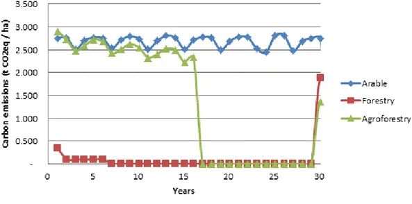
Figure 14 shows the changes in the annual carbon emissions in the arable, forestry and silvoarable systems in Bedfordshire, United Kingdom. The arable system shows the highest carbon emissions followed by the silvoarable and the forestry systems. During the first sixteen years the carbon emissions of the arable and silvoarable systems are very similar. However, after year sixteen there is no longer a crop component in the silvoarable system and consequently, the annual emissions are notably reduced.
Figure 14. Modelled carbon emissions associated with machinery use from an arable, silvoarable and forestry system in Bedfordshire, United Kingdom
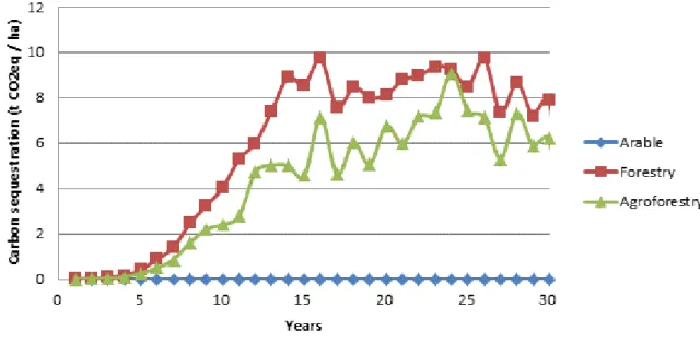
Figure 15 shows the change in the potential annual carbon sequestration of the arable, forestry and agroforestry systems in Bedfordshire, United Kingdom. The forestry system shows the highest carbon
y = 0.2149x + 23.621 0 10 20 30 40 50 0 25 50 75 100 Fu e l c on s um pti on (L ha -1)
Proportion of clay in soil (%)
y = 0.0052x + 1.0029 0.0 0.4 0.8 1.2 1.6 2.0 0 25 50 75 100 Wo rk rate (h ou rs ha -1)
Modelling the economics of agroforestry www.agforward.eu sequestration followed by the agroforestry and the arable systems. For the arable system, it was assumed that there is no annual carbon sequestration because all sequestered carbon is in effect released shortly after production and use of the products.
Figure 15. Modelled annual sequestered carbon for an arable, agroforestry, and forestry system in Bedfordshire, UK
Figure 16 shows the annual carbon emissions in the arable, forestry and agroforestry systems in Schwarzbubenland, Switzerland. The arable system shows the highest carbon emissions followed by the agroforestry and the forestry systems.
Figure 16. Modelled annual carbon emissions for the arable, agroforestry and forestry systems in Schwarzbubenland, Switzerland
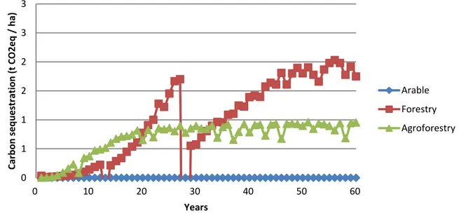
Figure 17 shows the change in the potential annual carbon sequestration of the arable, forestry and agroforestry systems in Schwarzbubenland, Switzerland. The forestry system shows the highest
0.500 1.000 1.500 2.000 2.500 3.000 3.500 0 10 20 30 40 50 60 Car b o n e m issi o n s (t CO2eq / h a) Years Arable Forestry Agroforestry
carbon sequestration followed by the agroforestry and the arable systems. In the forestry system, a thinning in year twenty-eight produces a sharp decrease in the quantity of sequestered carbon.
Figure 17. Modelled annual sequestered carbon for the arable, agroforestry and forestry system in Schwarzbubenland, Switzerland 0 1 1 2 2 3 3 0 10 20 30 40 50 60 Car b o n seq u e str ation (t C O2eq / h a) Years Arable Forestry Agroforestry
Modelling the economics of agroforestry www.agforward.eu 3.3.2 Soil erosion losses
Soil erosion losses can be evaluated using of the Revised Universal Soil Loss Equation (RUSLE) (Equation 1), which is frequently used to calculate the annual soil loss in different production systems. The RUSLE equation is described as:
A = R * K * LS * C * P (Equation 1)
Where A is the estimated average soil loss in tons per acre per year; R is the rainfall-runoff erosivity factor; K is the soil erodibility factor; L is the slope length factor; S is the slope steepness factor; C is the cover-management factor; P is the support practice factor.
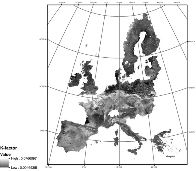
When comparing soil loss in arable, forestry and silvoarable systems in the same geographical area, the factors R, K, LS and P were considered to be the same and only changes in the C-factor were used to assess the differences among the systems. Figure 18 shows the K factor values used in Farm-SAFE to calculate soil erosion losses.
Figure 18. K factor values used in Farm-SAFE to calculate soil erosion losses by water through the RUSLE equation (Source: European Soil Data Centre, http://esdac.jrc.ec.europa.eu/).
K-factor Value High : 0.0766097 Low : 0.00469355 K-factor Value High : 0.0766097 Low : 0.00469355 50°0'0"E 40°0'0"E 30°0'0"E 20°0'0"E 20°0'0"E 10°0'0"E 10°0'0"E 0°0'0" 0°0'0" 10°0'0"W 10°0'0"W 20°0'0"W 30°0'0"W 60°0'0"N 60°0'0"N 50°0'0"N 50°0'0"N 40°0'0"N 40°0'0"N
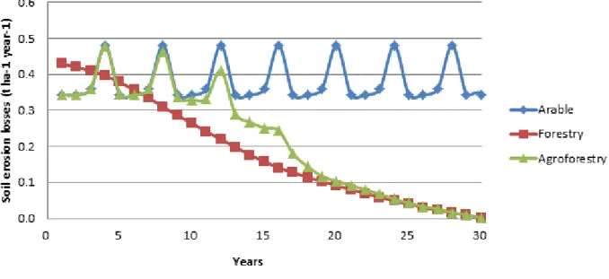
Figure 19 and Figure 20 show the modelled soil erosion losses (annual and cumulative) for each land use in Bedfordshire.
Figure 19. Modelled annual soil erosion losses by water for the arable, agroforestry and forestry system in Bedfordshire, UK
Figure 20. Modelled cumulative soil erosion losses by water for the arable, agroforestry and forestry system in Bedfordshire, UK
Modelling the economics of agroforestry www.agforward.eu 3.3.3 Nitrogen and phosphorus surplus
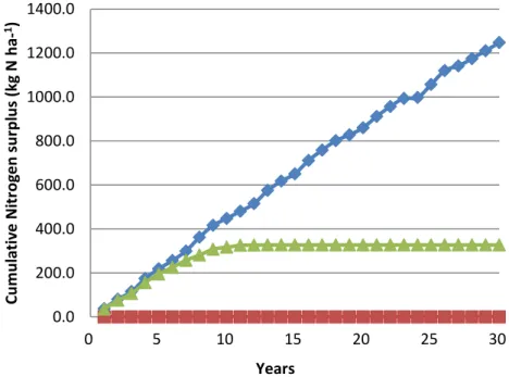
The emissions of Nitrogen (N) and Phosphorus (P) have been incorporated in the assessment of Farm-SAFE. The differences among arable, forestry and silvoarable systems are calculated as a function of the N and P fertilizer rates and the N and P leaching rates of each system. Figure 21 and Figure 22, show the nitrogen surplus in the case study for Bedfordshire (UK). Figure 23 and Figure 24, show the phosphorous surplus in the same case study.
Figure 21. Modelled annual nitrogen surplus for the arable (blue line), agroforestry (green) and forestry (red) systems in Bedfordshire, UK
Figure 22. Modelled cumulative nitrogen surplus for the arable (blue line), agroforestry (green line) and forestry (red line) systems in Bedfordshire, UK
0.0 10.0 20.0 30.0 40.0 50.0 60.0 70.0 80.0 0 5 10 15 20 25 30 N itr o ge n su rp lu s (k g N h a -1ye ar -1) Years Arable Forestry Agroforestry 0.0 200.0 400.0 600.0 800.0 1000.0 1200.0 1400.0 0 5 10 15 20 25 30 Cu m u lativ e N itr o ge n su rp lu s (k g N ha -1) Years Arable Forestry Agroforestry
Figure 23. Modelled annual phosphorus surplus for the arable (blue line), agroforestry (green line) and forestry (red line) systems in Bedfordshire, UK
Figure 24. Modelled cumulative phosphorus surplus for the arable (blue line), agroforestry (green line) and forestry (red line) system in Bedfordshire, UK
0.0 2.0 4.0 6.0 8.0 10.0 12.0 14.0 16.0 18.0 0 5 10 15 20 25 30 Ph o sp h o ru s su rp lu s (k g P h a -1 ye ar -1 ) Years Arable Forestry Agroforestry 0.0 50.0 100.0 150.0 200.0 250.0 300.0 350.0 400.0 0 5 10 15 20 25 30 Cu m u lativ e Ph o sp h o ru s su rp lu s (k g P ha -1) Years Arable Forestry Agroforestry
Modelling the economics of agroforestry www.agforward.eu 3.4 Economic analysis
Whilst the financial analysis aimed to show a plot-level profitability indicator from a farmer perspective the economic analysis attempted to provide a plot-level profitability indicator from a societal perspective. The economic appraisal built upon the NPVF (see Equation 1) and included
benefits and costs from the five environmental externalities converted into monetary terms (EEt) in
each year t. The NPV for the economic appraisal (NPVE) was denoted as:
𝑁𝑃𝑉𝐸 = ∑ (((𝑅𝑡− 𝑉𝐶𝑡− 𝐹𝐶𝑡) (1 + 𝑖)𝑡 ) + ( 𝐸𝐸𝑡 (1 + 𝑗)𝑡)) 𝑛 𝑡=0 𝐸𝑞. (3)
where j is the assumed discount rate for environmental costs and benefits (which was assumed to be 4% as in the financial analysis). From the NPVE, the economic EAV was calculated as in Equation 2.
The final goal of Farm-SAFE is to allow the end-user to assess the financial and economic profitability of the different land uses. In doing so, Farm-SAFE first quantifies the environmental externalities using the different indicator units and subsequently, converts them into monetary terms.
3.4.1 The case study of Bedfordshire, United Kingdom
Figure 25 shows the quantified environmental externalities and how much they represent in monetary terms at the end of the rotation age in Bedfordshire (30 years).
Figure 25. The quantity and derived economic value of five environmental externalities (GHG emissions, carbon sequestration, soil erosion, nitrogen surplus, and phosphorus surplus) for the arable, silvoarable and forestry for the case study in Bedfordshire case study, UK
Figure 26 shows the results of the financial and economic analysis in Bedfordshire, UK. As shown, including grants, agroforestry is the most profitable land-use system in the economic analysis, i.e. when the environmental externalities are internalised.
Quantified EE in different units
Converted EE in economic terms (€ ha
-1)
0 400 800 1200 a ) G H G e m is s io n s ( t C O 2 e q /h a ) b ) C a rb o n s e q u e s tr a ti o n ( t C O 2 e q /h a ) c ) S o il e ro s io n ( t s o il /h a ) d ) N it ro g e n s u rp lu s ( k g N /h a ) e ) P h o s p h o ru s s u rp lu s ( k g P /h a ) En v . e x te rn a li ti e s i n 3 0 y e a rs (d if . u n it s ) Landuse Arable Forestry Silvoarable -5000 -2500 0 2500 a ) G H G e m is s io n s b ) C a rb o n s e q u e s tr a ti o n c ) S o il e ro s io n d ) N it ro g e n s u p lu s e ) P h o s p h o ru s s u p lu s En v iro n m e n ta l e x te rn a li ti e s i n 3 0 y e a rs (EU R / h a ) Landuse Arable Forestry Silvoarable 0 250 500 750 1000 a ) G H G e m is s io n s ( t C O 2 e q /h a ) b ) C a rb o n s e q u e s tr a ti o n ( t C O 2 e q /h a ) c ) S o il e ro s io n l o s s e s ( t s o il /h a ) d ) N it ro g e n l e a c h in g ( k g N /h a ) En v . e x te rn a li ti e s i n 3 0 y e a rs (d if . u n it s ) Landuse Arable Forestry Silvoarable
A B
Figure 26. Comparison of A) the cumulative financial net margin of the arable, agroforestry and forestry system with B) an economic analysis of the same systems including five externalities for the case study in Bedfordshire, UK
Table 8 shows the EAV of the arable, forestry and silvoarable systems in Bedfordshire, including the GHG emissions in the economic assessment. The carbon price used for the calculations is 7.63 € per tonne of CO2 which can be obtained by farmers in the UK (UK Forestry Commission, available at:
www.forestry.goc.uk/carboncode). It is worth noting that this is a very conservative value, and other values, such as mitigation values and social cost values are higher. As shown, the forestry system has the lowest GHG emissions and the highest potential for sequestration. Internalising GHG emissions reduces the difference in the economic profitability between the arable system and the forestry and silvoarable system. Starting from the assumption of no grants, the inclusion of the societal cost of GHG emissions reduces the difference between the EAV of the arable and the silvoarable system from 242 € ha-1 to 159 € ha-1. These results highlight how including environmental costs can change the relative societal advantage of different land uses.
Table 8. Equivalent Annual Value (EAV) of an arable, forestry and silvoarable system in Bedfordshire in the United Kingdom. Results shown for a time horizon of 30 years at a 5% discount rate.
Arable1 Silvoarable2 Forestry3
EAV with grants (€ ha-1 year-1) 561 467 131
EAV without grants (€ ha-1 year-1) 314 72 -17
Emissions of CO2eq in 30 years (t CO2eq ha-1) 81 42 3
EAV of CO2eq emissions (€ ha-1 year-1) -40 -21 -1
Potential sequestration of CO2eq in 30 years (t CO2eq ha-1) 0 129 177
EAV of CO2eq potential sequestration (€ ha-1 year-1) 0 64 88
EAV with grants and GHG externalities (€ ha-1 year-1) 521 510 218
EAV without grants and GHG externalities (€ ha-1 year-1) 274 115 70
1
: the arable system was a rotation of wheat, wheat, barley and oilseed rape
2
: the silvoarable system was the same rotation as the arable system with poplar hybrids planted at 113 trees per hectare.
3
: the forestry system was hybrid poplars planted at a density of 156 trees per hectare.
Economic analysis (societal
perspective)
Financial analysis (farmer’s
perspective)
-6000 -4000 -2000 0 2000 4000 6000 8000 10000 0 10 20 30 Cu m u lativ e N e t M ar gi n ( € / h a) Years Arable: wheat-wheat-barley-oilseed Forestry: hybrid poplarAgroforestry: hybrid poplar with wheat-wheat-barley-oilseed
-6000 -4000 -2000 0 2000 4000 6000 8000 10000 0 5 10 15 20 25 30 Fi n an ci al Cu m u lativ e N e t M ar gi n ( € ha -1) Years Arable Forestry Agroforestry -6000 -4000 -2000 0 2000 4000 6000 8000 10000 0 5 10 15 20 25 30 Ec o n o m ic C u m u lativ e N e t M ar gi n ( € ha -1) Years Arable Forestry Agroforestry
Modelling the economics of agroforestry www.agforward.eu 3.4.2 The case study of Schwarzbubenland, Switzerland
An economic assessment was also used in the Schwarzbubenland case study. The approach was similar to the one used in the Bedfordshire case study but only GHG emissions and above-ground carbon sequestration were included in the assessment. Table 9 shows the EAV of the arable, forestry and silvoarable systems in Switzerland, including the GHG emissions in the economic assessment. As in the Bedfordshire case study the arable system has the highest carbon emissions and the lowest rate of carbon sequestration. With grants, the agroforestry system is the most profitable land use (with and without GHG emissions). However, without grants, it is the least profitable land use (with and without the GHG emissions).
Table 9. Equivalent Annual Value (EAV) of an arable, forestry and silvoarable system in
Schwarzbubenland, Switzerland. Results shown for a time horizon of 60 years at a 5% discount rate.
Arable1 Agroforestry2 Forestry3
EAV with grants (€ ha-1 year-1) 1,359 1,450 303
EAV without grants (€ ha-1 year-1) -734 -1,354 -789
Emissions of CO2eq in 60 years (t CO2eq ha-1) 137 52 3
EAV of CO2eq emissions (€ ha-1 year-1) -55 -21 -1
Potential sequestration of CO2eq in 60 years (t CO2eq ha-1) 0 42 50
EAV of CO2eq potential sequestration (€ ha-1 year-1) 0 17 20
EAV with grants and GHG externalities (€ ha-1 year-1) 1,303 1,515 322
EAV without grants and GHG externalities (€ ha-1 year-1) -789 -1,359 -770
1: the arable system was a rotation of oilseed rape, wheat, grassland and wheat 2
: the agroforestry system was grassland with cherry tree for fruit production planted at 80 trees per hectare.
3
4
Modelling and valuing the environmental impacts of arable, forestry and agroforestry
systems: a case study
This is the pre-submission version of the following paper which has been published in Agroforestry Systems. The following citation should be used for this paper: García de Jalón, S., Graves, A., Palma, J.H.N., Williams, A., Upson, M.A., Burgess, P.J. (2017). Modelling and valuing the environmental impacts of arable, forestry and agroforestry systems: a case study. Agroforestry Systems DOI: 10.1007/s10457-017-0128-z
4.1.1 Abstract
The use of land for intensive arable production in Europe is associated with a range of externalities that typically imposes costs on third parties. The introduction of trees in arable systems can potentially be used to reduce these costs. This paper assesses the profitability and environmental externalities of a silvoarable agroforestry system, and compares this with the profitability and environmental externalities from an arable system with no trees and a forestry system. A silvoarable experimental plot of poplar trees planted in 1992 in Bedfordshire, Southern England, was used as a case study. The Yield-SAFE model was used to simulate the growth of the silvoarable, arable, and forestry land uses along with the associated environmental externalities, including carbon sequestration, greenhouse gas emissions, nitrogen and phosphorus surplus, and soil erosion losses by water. The Farm-SAFE model was then used to quantify the monetary value of these effects. The study assesses both the financial profitability from a farmer perspective and the economic benefit from a societal perspective. The arable system was the most financially profitable followed by the silvoarable and forestry systems. However, when the environmental externalities were included, silvoarable agroforestry provided the greatest societal benefit. This suggests that the appropriate integration of trees in arable land can provide greater well-being benefits to society overall, than either arable farming without trees, or the forestry systems alone.
4.2 Introduction
The objectives of the EU Common Agricultural Policy, in concise form, are to ensure i) viable food production, ii) balanced territorial development, and iii) sustainable management of natural resources, with a focus on greenhouse gas emissions, biodiversity, soil and water (Article 110 in EU, 2013). Silvoarable agroforestry (the integration of trees with arable production) is a land use practice that could help achieve these objectives.
Over recent decades, many agricultural systems in Europe have been simplified through intensification and mechanisation in order to reduce management cost and labour (Dupraz et al. 2005; Burgess and Morris, 2009, Quinkenstein et al. 2009), whilst at the same time becoming increasingly reliant on external inputs such as nutrients, pesticides, and machinery (Nemecek et al. 2011; Palma et al. 2007). These systems have enabled the competitive production of high quantities of safe and low cost food for consumers without the need to expand the area of agricultural land. However, many systems have resulted in significant negative environment costs that are borne by society as a whole, rather than individual producers or consumers. These costs, or externalities, include water pollution (leaching and runoff of nitrogen, phosphorus and pesticides), soil degradation (e.g. erosion, compaction and loss of soil organic matter and soil biodiversity), and greenhouse gas (GHG) emissions such as CO2 and N2O (Nemecek et al. 2011; Renzulli et al. 2015).
These environmental externalities are rarely accounted for in the profitability analysis of agricultural systems, since usually they have no market value.
Modelling the economics of agroforestry www.agforward.eu Various studies have found that environmental externalities from arable systems can be reduced by the appropriate integration of trees (Jose, 2009; Mosquera-Losada et al. 2011; Quinkenstein et al. 2009; Smith et al. 2012), such as the potential for mitigating climate change through carbon sequestration (Nair et al. 2009; Nair and Nair, 2014), reducing soil degradation (Graves et al. 2015), and reducing adverse impacts on water quality from agrochemical use (Nair, 2011a; Palma et al. 2007). However, whilst planting trees on arable land can help reduce environmental externalities, the uptake of silvoarable systems remains relatively slow. This could be a result of the cost of tree planting and management reducing immediate profitability and the uncertainty regarding the long-term financial benefits from harvesting mature trees. In the EU, efforts have been made to promote adoption of silvoarable systems through policy (Article 222) and projects such as SAFE (Dupraz et al. 2005) and AGFORWARD (Burgess et al. 2015) have been funded to provide scientific guidance on the costs and benefits of implementing silvoarable systems across Europe.
For long rotation systems such as agroforestry and forestry systems, modelling becomes essential. In recent years various biophysical models such as Hi-sAFe (Dupraz et al. 2004), SCUAF (Young et al. 1998), WaNuLCAS (van Noordwijk and Lusiana, 1999), and Yield-SAFE (Van der Werf et al. 2007) have been developed to simulate the growth and interaction of trees and crops in silvoarable systems. Some economic models have also been developed to assess the financial profitability of silvoarable systems. These for example, include ARBUSTRA (Liagre, 1997), Farm-SAFE (Graves et al. 2011), and POPMOD (Thomas, 1991).
The Farm-SAFE model (Graves et al. 2011) integrates the Yield-SAFE outputs with financial and economic analysis. Yield-SAFE simulates the biophysical growth of trees and crops, it can be adapted to quantify the impact of selected environmental externalities, and it can be used to determine the financial and economic impacts of different arable, silvoarable and forestry land uses. Within the AGFORWARD project, the Farm-SAFE model has been adapted to assess both the financial profitability from a farmer perspective and the economic profitability from a societal perspective. Using the adapted Farm-SAFE model, this paper evaluates and compares the biophysical development, financial profitability, and social impact of environmental externalities for arable, forestry, and silvoarable poplar systems to provide a more complete assessment of the societal benefits and costs of these land uses.
4.3 Methods and data
The methodological framework of this study is separated into five stages: i) simulation of the biophysical growth of trees and crops for the Bedfordshire case study, ii) assessment of financial performance, iii) quantification of the environmental externalities, iv) conversion of the environmental externalities into monetary terms, and v) assessment of full economic performance through inclusion of the environmental externalities in the analysis.
4.3.1 Bedfordshire case study
The case study is based on an experiment in Silsoe in Bedfordshire, England comprising 2.5 ha of silvoarable (poplar + cultivated crops) and forestry (poplar + fallow land) treatments surrounded by one hectare of conventionally cropped arable land (Burgess et al. 2005). The site is located in a relatively flat area at 59 m above mean sea level. The mean soil texture is 55% clay, 26% silt, and 19%
sand. Annual rainfall ranges from 410 mm to 867 mm and mean annual temperature from 9.1°C to 11.3°C.
Four poplar hybrid varieties, including Beaupré (Populus trichocarpa x P. deltoides), were planted in 1992. The four hybrids were planted at a spacing of 6.4 m in a North-South orientation along rows spaced 10 m apart. Tree height and diameter at breast height was measured at intervals until 2011, when the poplars were harvested, 19 years after planting (Upson, 2014). The arable crops from 1992 to 2003 included spring wheat, winter wheat, winter barley and spring beans; after 2003 the understorey reverted to grass (Burgess et al. 2005; Upson 2014).
4.3.2 Biophysical simulation
Because poor management led to crop failure in some years, a standardised crop rotation of wheat, wheat, barley and oilseed rape was assumed for the financial and economic analysis. The crop yields and the tree growth were simulated using the Yield-SAFE biophysical model (van der Werf et al. 2007) calibrated using the tree growth of the Beaupré hybrid and the relative crop yields obtained in the silvoarable system relative to the arable control (Burgess et al. 2005). Daily climatic data were retrieved from CliPick (Palma et al. 2015). In this way, crop and tree growth simulations were derived for three systems: i) a control arable system, ii) a silvoarable system (Beaupré at a density of 156 trees per hectare and arable cropping for 14 years), and iii) a forestry system (Beaupré at a density of 156 trees per hectare). The length of the tree rotation was specified as 30 years.
The modelled mean control crop yields of 8.78 t ha-1, 6.70 t ha-1 and 3.49 t ha-1 for wheat, barley and oilseed rape respectively are similar to mean yields reported for the UK by Agro Business Consultants (2015) (Figure 27a). The simulated crop yields in the silvoarable system (Figure 27b) declined as the tree canopy expanded, with the final crop grown 14 years after tree planting (i.e. three years longer than achieved in practice).
4.3.3 Financial analysis
The financial performance of arable, forestry and silvoarable system was assessed using Farm-SAFE (Graves et al. 2011) on the basis of the annual net margins per hectare. The net margin was calculated as revenues from harvested products (grain, straw, timber and firewood) and grants minus variable costs (e.g. crop seed, tree planting, fertiliser, crop and tree protection, pruning, thinning, cutting and other costs) and assignable fixed costs (e.g. installation and repairs of infrastructure, fuel and energy, machinery, insurance and labour and rented machinery costs). Because people generally prefer to receive goods and services in the present rather than the future, revenues and costs were discounted and converted into financial net present values (NPVF: € ha-1),
denoted using Equation 1: 𝑁𝑃𝑉𝐹= ∑ ((𝑅𝑡 − 𝑉𝐶𝑡− 𝐹𝐶𝑡) (1 + 𝑖)𝑡 ) 𝑛 𝑡=0 𝐸𝑞. 1
where Rt, VCt, and FCt were respectively revenue, variable costs, and assignable fixed costs in year t
(€ ha-1), i was the discount rate, and n was the time horizon for the analysis. A discount rate of 4% was chosen, as this is marginally above the discount rate of 3.5% used by the UK Government for cost-benefit analysis (HM Treasury, 2003). Although the costs were obtained in terms of pounds
Modelling the economics of agroforestry www.agforward.eu sterling, in this paper they are report in terms of Euros, assuming an exchange rate of £1 being equivalent to €1.389.
The financial profits of the different systems were compared in terms of a financial equivalent annual value (EAVF: € ha-1 year-1) using Equation 2:
𝐸𝐴𝑉𝐹= 𝑁𝑃𝑉𝐹( (1 + 𝑖)
𝑛
(1 + 𝑖)𝑛− 1) 𝑖 𝐸𝑞. 2
Financial data (Table 10) related to the crops were obtained from a 2015 farm management handbook (Agro Business Consultants, 2015), e.g. a wheat grain price of £125 t-1. The assumed crop prices were then assumed for the full rotation cycle. The grant receipts were based on the Basic Payment Scheme (BPS) for lowlands in England (235 € ha-1 yr-1) also in 2016.
Table 10. Assumptions for crop revenues and costs in the analysis Crop Grain price (€ t-1) Seed rate (kg ha-1)
Fertiliser rate Variable
costs1 (€ ha-1) Fixed costs (exc. labour) 2 (€ ha-1) Labour costs (€ ha-1) (kg N ha-1) (kg P2O5 ha-1) (kg K2O ha-1) Wheat 174 160 175 60 55 653 444 162 Barley 160 155 145 55 40 653 444 146 Oilseed 361 5 200 55 45 535 444 151
(1) Includes seed, fertiliser, spray and other costs.
(2) Includes costs relating to fuel and repairs, machinery, interest on working capital, installation, rent and other fixed costs.
Table 11 shows the summary of costs for the tree component in the silvoarable and forestry system. The silvicultural management was based on Savill (1991) and the associated costs and labour inputs were derived from the experimental plot in the Bedfordshire case study (Graves et al. 2007). The woodland planting grant was considered only for the forestry system which as a wide-spaced broadleaved system was eligible for support (1888.90 € ha-1 paid upon completion in the first year and 472.20 € ha-1 yr-1 during the first five years (Agro Business Consultants, 2015)).
4.3.4 Modelling the environmental externalities 4.3.4.1 Greenhouse gas (GHG) emissions
A Life Cycle Assessment (LCA) model (Williams et al. 2010) was integrated into the Farm-SAFE model to measure GHG emissions in carbon dioxide equivalents (CO2e) associated with the manufacture
and use of machinery and agrochemicals. The analysis focused only on CO2 emissions and did not
consider N2O. In order to compare the arable, forestry and silvoarable systems, a functional unit of
one hectare was used in the analysis. Equation 3 shows the emissions that were included in the LCA: 𝐸𝑚𝑖. 𝐶𝑂2𝑒𝑡 = 𝑀𝑚+ 𝑀𝑓+ 𝑀𝑝+ 𝐹 𝐸𝑞. 3
where Emi.CO2et is the total emitted GHG (t CO2e ha-1 yr-1) in year t, and other factors include the
emissions from the manufacture of field machinery (Mm), fertiliser (Mf) and pesticides (Mp) and the
emissions associated with the fuel used for field operations (F). For the arable system and silvoarable intercrop area, machinery operations included cultivation, agrochemical application, harvesting and baling. In the forestry system and the tree component of the silvoarable system, the machinery operations included site preparation (ground preparation, full weeding, marking out, planting, tree protection and grass sward establishment), agrochemical application (localised weeding) and
harvesting (pruning, epicormics removal, grass sward maintenance and clear felling). Nursery costs were not included. The GHG emissions of the silvoarable system were calculated by adding the GHG emissions of the intercrop area and the tree component area together. Emissions from manufacture of machinery was based on a per hectare utilisation rate calculated from the estimated life expectancy of the machinery (Nix, 2014). Emissions from manufacturing field diesel, fertiliser, and pesticides were calculated from the per hectare quantities used. Emissions to the atmosphere from field diesel, fertiliser, and pesticides were also traced back to the quantities used.
Table 11. Summary of costs associated with the tree component of the systems.
Tree operations Units Forestry Silvoarable
Establishment cost (total) (€ ha-1) 753.28 753.28
Costs of individual plants (€ tree-1) 1.33 1.33 Costs of individual tree protection (€ tree-1) 0.27 0.27 Costs of tree mulch (€ tree-1) 0.40 0.40 Costs of ground preparation (€ ha-1) 48.93 48.93 Labour for planting trees (min tree-1) 3.00 3.00 Labour for tree protection (min tree-1) 0.40 0.40 Labour for tree mulch (min tree-1) 1.70 1.70
Weeding cost (total) (€ ha-1) 10.40 22.93
Single herbicide for tree row (min m-2) 0.08 0.00 Annual cost of herbicide (€ tree-1) 0.00 0.002 Removal of mulch (min tree-1) 1.50 0.00 Grass cut between tree rows (€ ha-1) 0.00 20.00 Labour to establish grass sward (min m-2) 0.50 0.00 Labour to maintain grass sward (min m-2) 0.30 0.00 Labour to tree maintenance (min tree-1) 1.20 1.20
Pruning cost (total) (€ ha-1) 805.06 805.06
Height first prune (m) 1.00 1.00
Labour first prune (min tree-1) 1.00 1.00
Height last prune (m) 8.00 8.00
Labour last prune (min tree-1) 15.00 15.00 Removal of prunings (min tree-1) 4.00 4.00
Harvest cost (total) (€ ha-1) 583.96 583.96
Tree cutting (min tree-1) 7.00 7.00
Admin. and insurance and other cost (total) (€ ha-1) 90.00 90.00
Administrative, insurance and tax cost (€ ha-1) 9.00 9.00 Average annual maintenance costs (€ ha-1 year-1) 51.28 51.40
A ‘cradle-to-field gate’ approach was applied i.e. emissions associated with grain drying, crop storage and downstream processing were excluded. The construction of farm infrastructure was also excluded. The GHG emissions from land-use change were not included.
4.3.4.2 Aboveground-biomass carbon sequestration
Estimates for aboveground carbon sequestration were obtained from the simulated tree growth. It was assumed that the carbon sequestered by the arable crops and tree branches would be quickly lost to the atmosphere after harvest and hence they were excluded from the analysis. Equation 4 was used to convert the simulated biomass into carbon dioxide equivalent sequestration (t CO2e ha-1
yr-1):
𝑆𝑒𝑞. 𝐶𝑂2𝑒𝑡= 0.50 𝛽𝑡𝑖𝑚𝑏𝑒𝑟,𝑡∗𝐴𝑡𝑜𝑚𝑖𝑐 𝑤𝑒𝑖𝑔ℎ𝑡 𝐶𝑂2
𝐴𝑡𝑜𝑚𝑖𝑐 𝑤𝑒𝑖𝑔ℎ𝑡 𝐶 𝐸𝑞. 4
where Seq.CO2et was the sequestered carbon dioxide equivalent (t CO2e ha-1 yr-1) in time t, where