OIL SPILL MODELING OFF THE BRAZILIAN EASTERN COAST: THE EFFECT OF TIDAL CURRENTS ON OIL FATE

OIL SPILL MODELING OFF THE BRAZILIAN EASTERN COAST:

THE EFFECT OF TIDAL CURRENTS ON OIL FATE

Angelo Teixeira Lemos

_{, Ivan Dias Soares}

_{, Renato David Ghisolfi}

_{and Mauro Cirano}

Received on May 26, 2009 / Accepted on November 23, 2009

ABSTRACT.This study presents a comparative analysis of several theoretical oil spill scenarios occurring in the vicinity of the Abrolhos Reefs, a preservation area located off the Brazilian east coast. The following petroleum blocks were considered in the study: BM-CUM-1, BM-CUM-2, J-M-259 and ES-M-418, to verify the effect of the tide on the oil spreading on the continental shelf in the eastern Brazilian. The probabilistic oil spill simulations were carried out for 30 days and considered an oil of intermediate API (American Petroleum Institute) type. The simulations were performed by the OSCAR (Oil Spill Contingency and Response) model which was fed by synoptic wind data and hydrodynamic data simulated by the POM (Princeton Ocean Model) model. Two distinct seasonal scenarios were studied: the austral winter and the austral summer of 1989 and the results were discussed in terms of seasonal variability caused by the winter/summer winds and differences in mesoscale instabilities. The effect caused by tidal currents was analyzed through the comparison between simulations with and without the tides. It was concluded that the tide strongly influenced the probabilistic results of fate of oil in the spill scenarios. Many factors have influenced this fate of the spreading of oil in the absence of supra-inertial processes, such as the location of the spill, the behavior of the prevailing winds and tides in the region. The tide absence in the hydrodynamic data did not found the worst case scenarios of the spill in simulations in blocks BM-CUM-1, BM-CUM-2 and J-M-259, mainly in summer with use of intermediate oil, underestimating the real scenarios of spill.

Keywords: tide, modeling, oil, POM, OSCAR.

RESUMO.O presente estudo teve por objetivo realizar modelagens de diferentes cen´arios de derramamentos de ´oleo em blocos de petr´oleo (BM-CUM-1, BM-CUM-2, J-M-259 e ES-M-418) em ´areas adjacentes ao Recife de Abrolhos, a fim de verificar o efeito da mar´e no espalhamento do ´oleo na plataforma leste brasileira. Foram realizadas simulac¸˜oes de 30 dias de derramamento de ´oleo de grau API (American Petroleum Institute) intermedi´ario, utilizando como ferramenta o modelo OSCAR (Oil Spill Contingency and Response), sendo alimentado com dados hidrodinˆamicos simulados pelo modelo POM (Princeton Ocean Model) e dados de vento sin´otico simulados pelo modelo ETA, o qual foi alimentado com dados de rean´alise do NCEP. Os per´ıodos abordados foram o inverno e o ver˜ao do ano de 1989 e os resultados foram discutidos em termos das variac¸˜oes de intensidade e direc¸˜ao do espalhamento causado pelo vento sin´otico de cada estac¸˜ao, assim como pelos processos de mesoescala e pela mar´e. O efeito causado pela mar´e foi analisado atrav´es da comparac¸˜ao de simulac¸˜oes com e sem mar´e. Concluiu-se que a mar´e influenciou fortemente nos resultados probabil´ısticos de destino do ´oleo nos cen´arios de derramamento. Muitos fatores mostraram influenciar nesse destino do espalhamento do ´oleo com a ausˆencia dos processos supra-inerciais, como a localizac¸˜ao geogr´afica do derramamento, os ventos predominantes e o comportamento da mar´e na regi˜ao. A ausˆencia da mar´e nos dados hidrodinˆamicos n˜ao permitiu encontrar os cen´arios de pior caso de derramamento em simulac¸˜oes nos blocos BM-CUM-1, BM-CUM-2 e J-M-259, principalmente no ver˜ao com a utilizac¸˜ao de ´oleo intermedi´ario, subestimando os cen´arios reais de derramamento.

Palavras-chave: mar´es, modelagem, ´oleo, POM, OSCAR.

1Pesquisa e Simulac¸˜ao Sobre a Dinˆamica do Oceano (LabPosseidon), Universidade Federal do Esp´ırito Santo (UFES), Departamento de Oceanografia e Ecologia (DOC), Campus Goiabeiras, Av. Fernando Ferrari, 514, 29075-910 Vit´oria, ES, Brazil. Phone: +55(27) 4009-7787; Fax: +55(27) 4009-2500 – E-mails: angelole-mos@gmail.com; gringoghisolfi@gmail.com

2Laborat´orio de Experimentac¸˜ao Num´erica em Oceanografia (LENOC), Universidade Federal do Rio Grande (FURG), Instituto Oceanogr´afico, Campus Carreiros, Av. It´alia, km 8, 96201-900 Rio Grande, RS, Brazil. Phone: +55(53) 3233-6874; Fax: +55(053) 3233-6652 – E-mail: isoares@atlantis.org.br

3Centro de Pesquisas em Geof´ısica e Geologia (CPGG), Universidade Federal da Bahia (UFBA), Instituto de F´ısica, Departamento de F´ısica da Terra e do Meio Ambiente/ Grupo de Oceanografia Tropical, Campus Ondina, 40170-280 Salvador, BA, Brazil. Phone: +55(71) 3283-6686; Fax: +55(71) 3283-6681 – E-mail: mcirano@ufba.br

INTRODUCTION

The continental shelf off the Brazilian eastern coast hosts the lar-gest and the richest coral reefs in Brazil: The Abrolhos Coral Reefs. According to Le˜ao (1999), the Abrolhos Coral Reefs are signifi-cantly different from most of the coral reefs described in the spe-cialized literature. The main differences are related to the morpho-logy of the reef structures, the type of bottom sediments and more importantly the coral organisms themselves. Although the Abro-lhos Coral Reefs show the highest species diversity found in Bra-zilian reefs, the number of species is four times smaller than in reefs located in the North Atlantic. Moreover many of the species found in the Abrolhos Coral Reefs are endemic and archaic, being originated from the Tertiary Age species, which became adapted to the stress caused by the Brazilian high turbidity waters (Le˜ao, 1999). The Abrolhos Coral Reefs are very sensitive to human-related stresses, especially those human-related to the oil industry thus requiring special attention in policies designed to regulate oil ex-ploitation in Brazilian waters.

The Abrolhos Reefs are located in a topographic complex area which includes the Abrolhos Bank, the Royal Charlotte Bank, the Vit´oria-Trindade Ridge and several submerse mounts (Fig. 1). Ac-cording to Campos (1995) the local hydrodynamics is strongly influenced by this complex topography and topographically indu-ced meanders and eddies are features commonly observed asso-ciated with the Brazil Current in this area. Schmidt (2004) showed that the Brazil Current mesoscale processes are important to the local circulation, being responsible for significant water mass ex-changes between shallow and deep waters. The continental shelf at the Abrolhos Bank is nearly 200 km wide (Zembruscki, 1979) which, according to Schmidt (2004), allows for the evolution of topographically induced eddies. Coastal capes such as the Cabo Frio Cape and S˜ao Tom´e Cape are also strong conditionings for the local hydrodynamics, causing the formation of cyclonic and anticyclonic eddies (Silveira et al., 2000a).

The thermohaline vertical structure at the slope and at the adjacent deep ocean includes the Tropical Water (TW) from sur-face to 100 m, the South Atlantic Central Water (SACW) in sub-surface layers, between 100 m and 500 m, the Antarctic Inter-mediate Water (AAIW) from 500 m to 1200 m and the North Atlantic Deep Water (NADW) and Antarctic Bottom Water (AABW) in very deep layers (e.g. Stramma & England, 1999; Silveira et al., 2000b, Cirano et al., 2006). The baroclinic modes associa-ted with this intricate vertical water mass distribution originates both stationary and moving instabilities, which grow into mean-ders and eddies (Soares, 2007). A known mesoscale phenomena

is the Vit´oria Eddy, which was first described by Schmid et al. (1995) as a permanent feature. Gaeta et al. (1999) also descri-bed the Vit´oria Eddy as a permanent, topographically-induced fe-ature, which has strong influence in the local biota as it controls nutrient distribution.

It is within this rich environment that oil exploitation is growing very fast, mainly due to the light oil found in the area compared to those found in the Campos and Santos Basin, the most productive oil basins in Brazil. Prior to the oil exploitation, Oil Companies are obligated to conduct environmental studies, which use oil models to simulate oil spill drift and fate. These mo-dels range from simple Lagrangian momo-dels, simulating oil particle trajectories only, to fully three-dimensional models, which simu-late 3-D oil spills, as well as contingency, response actions and biology. They are very useful in determining the Activity Influence Area since they allow for oil spill mapping, both deterministically and probabilistically. In this study, we used the OSCAR (Oil Spill Contingency and Response) model, which was developed by the Norwegian SINTEF Group (Stiftelsen for INdustriell og TEknisk Forskning ved NTH– Foundation for Industrial and Technical Re-search) (Reed et al., 1999).

Several oil studies have used the OSCAR model for contin-gency planning, as well as for investigation of environmental sen-sitivity to oil contamination. Reed et al. (1995) studied small oil spills (<500 m3_{), resulting from two types of oil, occurring}

un-der different environmental conditions. They obtained satisfactory results in terms of the time necessary for containing the spillage when contingency equipment and personnel were in action. Aamo et al. (1997) conducted 48 different simulations with OSCAR to evaluate environmental sensitivity and concluded that in calm wa-ters the rescue operations were more efficient in recovering spilled oil than in offshore areas, where the wind was stronger. Reed et al. (2004) studied the use of dispersive chemicals in oil spills in Ma-tagorda Bay, Texas, using different oil spill scenarios and obser-ving the oil model efficiency, especially in terms of oil-sediment interaction.

Oil models can be used in either a probabilistic or a deter-ministic mode. The former results in probabilistic scenarios of certain property, such as the probability for the oil spill to re-ach the coastline. The probability is calculated from a number of short-term deterministic simulations, which are chosen randomly within a longer period of available simulation data. The probabi-listic simulations have the advantage of considering a larger range of variations of the forcing agents (winds, ocean currents, waves) since they consider a larger number of scenarios. Determinis-tic simulations, on the other hand, are used for a specific

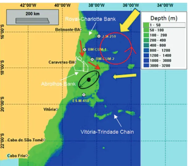
scena-Figure 1 – Study area and main oceanographic processes influencing the fate of oil in the region. The red arrows indicate the

Brazil Current, the red circle represents the Royal Charlotte Eddy, the black ellipse is tidal ellipses, the yellow arrows indicate the direction and intensity of prevailing wind. The circumscribed “x” are the locations of the oil blocks, whose names are printed in yellow on the figure. In green are bathymetric contours. The white line polygons are the protection areas, the APA Ponta das Baleias (larger polygon) and the buffer zones surrounding the Abrolhos National Park (Buffer Zone 1 to the north and Buffer Zone 2 to the east).

rio, for example the one which resulted in the largest volume of oil reaching the coastline. Besides, deterministic simulations can consider contingency strategies, because they conduct only one simulation.

In this study, we used the OSCAR model in a probabilistic mode to simulate oil spills resulting from theoretical accidents oc-curring in the surroundings of the Abrolhos Bank. Our main goal was to demonstrate that the oil model results are very sensitive to the quality of the hydrodynamic data that has been used to feed the oil model. We used two datasets, one with and another without the incorporation of tidal variability and our analysis focus on the influenced caused by the tidal currents on the oil spill fate. The text is organized in following sections. After the short literature review and the importance of the study presented in this introduc-tion, we present the study area in section 2. The methodology used for the hydrodynamic and the oil simulations is presented in section 3 and the results of both models are shown in section 4.

A discussion of the importance of the tidal currents for the oil drift is presented in section 5. Finally, the conclusions are presented in section 6.

STUDY AREA

Our study domain is located off the Brazilian eastern coast, in tro-pical latitudes, being limited northwards at the latitude of 15◦_S

and southwards at 23◦_{S. The domain, as well as a schematic}

drawing of all the forcing mechanisms (tidal currents, boundary currents and winds) is shown in Figure 1. In this figure we also show the locations of the oil spills (a “x” circumscribed by bo-xes) and the location of the Preservation Areas (the polygons li-mited by white lines). The oil spills were placed in areas so-called “oil blocks”, term used and named by the Agency ANP (Agˆencia Nacional do Petr´oleo, G´as Natural e Biocombust´ıveis). The exact locations are summarized in Table 1. All spills modeled here are theoretical, since no spill has ever occurred in the area. The

Table 1 – Geographic location of ANP oil blocks, where oil spills where placed.

Block Bight Latitude Longitude Depth (m) BM-CUM-1 Cumuruxatiba –17◦₀₀0₀₀00 _–38◦₄₁0₁₅00 ₁₀₄

BM-CUM-2 Cumuruxatiba –17◦₃₂0₃₀00 _–38◦₁₅0₀₀00 ₈₆

J-M-259 Jequitinhonha –16◦₁₅0₀₀00 _–37◦₅₂0₀₀00 _1.17

ES-M-418 Esp´ırito Santo –19◦₃₀0₀₀00 _–38◦₄₅0₀₀00 ₆₉

Preservation Areas are the “APA Ponta das Baleias”, the largest polygon in Figure 1, and the Abrolhos National Park (PARNA), which is split into two smaller polygons, named “Buffer Zones”.

The domain is large and is influenced by both shallow and deep water circulation. Tidal currents are stronger over the Banks reaching their highest values on the Abrolhos Bank, where the tidal ellipses have their longer axis oriented in the northe-ast/southwest direction, resulting in cross-shelf tidal currents (Lemos, 2006). The locally induced wind driven currents have a residual component, which is driven by the prevailing winds, while short-period variations are forced by the atmospheric fron-tal systems. The prevailing winds blow mostly from the northeast and from the east and according to Lessa & Cirano (2006), who analyzed onshore wind data sampled in the southern Bahia co-ast, the northeast1_{winds account for 30% of all cases, followed}

by east winds (24%) and then south and north winds (14% and 12%, respectively).

Seasonal variations of the prevailing winds occur due to vari-ations in the intensity and positioning of the South Atlantic At-mospheric High Pressure System (SAHP), which are in phase with the latitudinal migrations of the Inter-Tropical Convergence Zone (ITCZ). During the austral summer, the ITCZ is displaced southwards and the SAHP is stronger and larger, resulting in stronger northeast winds along the Brazilian eastern coast. Du-ring the opposite phase (austral winter), the ITCZ is displaced northwards, the SAHP is weaker and so are the northeast winds (Castro & Miranda, 1998). At synoptic timescales the most sig-nificant wind events occur during the austral autumn and win-ter seasons (Lessa & Cirano, 2006) when the atmospheric cold fronts are more intense and the southwest and southeast wind events are more frequent, in phase with the weak-northeast-prevailing-wind season.

As a consequence, the inner and mid shelves currents are ex-pected to have a residual wind driven component which is direc-ted southwestward, due to the prevailing northeast winds, as well as short-term variability forced by the atmospheric frontal sys-tems which cause current reversals at time scales of a few days.

At the supra-inertial frequency band, the tides are responsible for strong cross-shelf currents in the central part of the domain.

On the outer shelf and on the slope, the Brazil Current (BC), the western boundary current associated with the South Atlan-tic Sub-Tropical Gyre, is the dominant feature in the circulation. According to Silveira et al. (2000a) and Soutelino (2008) the BC originates at the latitude of 10◦_{S from the bifurcation of South}

Equatorial Current (SEC) and then flows southward. According to Cirano et al. (2006), the BC is very shallow at lower latitu-des and deepens as it flows poleward. Rodrigues et al. (2006) showed that the SEC bifurcation presents latitudinal migrations due to variation in the wind stress intensity, which result in sea-sonal variations in the BC volume and mass transports. When the ITCZ is displaced northwards (austral winter), the study area expe-riences weakened northeast winds and the SEC bifurcation moves northward. Therefore, in the austral winter season the BC trans-port is lower and the North Brazil Current, which is the northward current originated at the SEC bifurcation is enhanced. The op-posite occurs in the austral summer. A meandering pattern is permanently observed in the BC, as it flows at the offshore limit of the Abrolhos and the Royal Charlotte Banks, since the Banks themselves have a meander-like configuration.

METHODOLOGY

Because the domain experiences significant seasonal hydrody-namic variations, due to variations in wind stress and in the BC volume transport, our study was conducted in two distinct three-month-long periods, one spanning the austral summer and another spanning the austral winter of 1989. There is no particular reason why the year of 1989 was chosen, except for the fact that the hydrodynamic simulations were already done and ready to be used, thanks to another study previously conducted in the same area. Although this study focuses on the effect of tidal currents and these currents do not show significant seasonal changes, it is imperative to understand the low frequency current variability in order to discuss its contribution to the overall circulation and its impact in the oil spills. Our approach is to compare model

sults which contain the variability induced by all three forcing me-chanisms (winds, tides and the BC) against results which do not contain tidal-induced variability (only winds and the BC), seeking for modifications in size, shape, thickness and area of oil spills. We analyzed spills resulting from leakages of 192 m3_.day–1_,

oc-curring for 30 days, without contingency, in three different Basins: The Cumuruxatiba Basin, where we looked at blocks BM-CUM-1 and BM-CUM-2, the Jequitinhonha Basin (block J-M-259) and the Esp´ırito Santo Basin (block ES-M-418). These blocks were already licensed by the Agency ANP. The choice of 192 m3_.day–1

was done based on exploitations that are currently occurring in surrounding areas.

Wind data and hydrodynamic information are the input data necessary to carry out the probabilistic OSCAR simulations. The model simulation steps are summarized in Figure 2. The pro-babilistic oil simulations were conducted as randomly chosen 30-days simulations within the 90-days data period.

Hydrodynamic simulations

The hydrodynamic simulations were conducted with the Princeton Ocean Model (POM) (Blumberg & Mellor, 1987) and their con-figurations are summarized in Table 2. The data used as open boundary values are summarized below.

1. Temperature and salinity data used at the lateral open boundaries were obtained from the OCCAM Model (Ocean Circulation and Climate Advanced Modeling Project) glo-bal simulations with horizontal resolution of 1/4 of degree and 36 vertical levels (Webb et al., 1998). We used the monthly mean data which are available at the website of the OCCAM project (www.noc.soton.ac.uk/JRD/OCCAM). 2. Synoptic wind data with spatial resolution of 1/10 of

de-grees and time interval of 6 hours, produced by a local implementation of the ETA model, which was fed by the NCEP re-analysis data (Kalnay et al., 1996).

3. The tidal constituents M2, S2, N2, O1 and K1amplitude

and phase were obtained from the global simulation of the tide model FES95.2 (Le Provost et al., 1998), with spatial resolution of 1/2 of degree.

All simulations started from the rest and required a warm up period to allow the baroclinic currents to adjust to the OCCAM thermohaline fields. These warm up simulations were carried out previously to the 90-days simulations used to force the oil mo-del and are not considered in our analysis. The surface elevation data used at the open boundaries are a linear combination of the

OCCAM SSH values and the elevation computed (hourly) from the tidal constituents. The open boundary temperature and sali-nity values were updated monthly, but were linearly interpolated daily. The hydrodynamic data were stored at intervals of two hours and in four sigma levels.

The hydrodynamic model used a curvilinear grid, with higher spatial resolution near the coastal and shallow regions. The grid resolution ranged from nearly 1 km near the coast to 16 km offshore. In order to be used by the oil model these data had to be interpolated both horizontally and vertically. In the vertical, a linear interpolation was performed to compute the velocities at z-levels of 5 m, 20 m, 80 m and 300 m, since the hydrodynamic data were originally distributed in sigma levels. In the horizon-tal, the velocity data were interpolated, at each level, to a regular 91 × 91 grid with resolution of 10 km.

The wind data, which were distributed on a regular grid with spatial resolution of 1/10 of degree (oriented in the north-south direction), had to be vectorially-interpolated to be used in the cur-vilinear grid of the hydrodynamic model, but not to the oil model grid that is also regular.

Simulations with and without tides

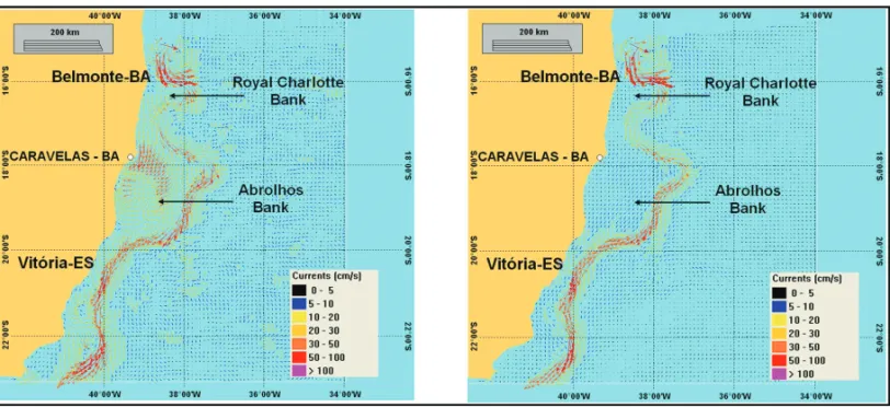
In order to obtain the hydrodynamic data that does not contain the tidal variability, the hydrodynamic data were low-pass filte-red using a Lanczos-cosine filter, with a time window of 40 hours, and the low-passed data were also stored at intervals of two hours. This resulted in four hydrodynamic data files, two containing the low-frequency and the tidal variability (summer and winter) and two containing only the low-frequency variability. These are the data files which were used (together with the wind data file) to feed the oil model. In Figure 3 we present two snapshots of ocean cur-rents at the 5 m depth during the summer simulation, one with the tides (left hand panel) and another without the tides (right hand panel). The tidal currents may be seen very clearly on the continental shelf in the left hand panel but not on the right hand panel. In this snapshot, the tidal currents are seeing as across-shelf vectors directed onshore, but it is useful to remind that the tidal currents are frequently changing direction and subsequent plots, which are not shown, would have the tidal currents direc-ted offshore. It is also noticeable that the figure where low-passed filter was used, in the right hand panel, has only the BC and its mesoscale features, flowing poleward at the shelf break and very weak currents on the continental shelf.

Oil spill simulations

The oil spill simulations were carried out in probabilistic mode by the OSCAR model, having as input data the hydrodynamic data

Figure 2 – Flowchart of methodological steps.

Table 2 – Summary of parameters and configurations used in the hydrodynamic simulations.

Parameter Value

Time Step (external mode/internal mode) 8 sec / 240 sec

Grid Spacing Ranging between 1 km (near coastline) and 16 kms offshore Number of layers 22

Surface Elevation open boundary condition Blumberg & Kantha partially clamped condition External mode velocities open boundary condition Sommerfeld radiation condition

Internal mode velocities open boundary condition Orlanski radiation condition Temperature and Salinity open boundary condition POM Advective condition Surface Heat and Salt Fluxes None

Surface Momentum Fluxes Wind stress

Figure 3 – Summer period snapshots of ocean currents with (left hand side panel) and without (right hand side panel) the application of the 40h low-pass

files (with and without tides) and the wind data. The wind data were multiplied by 0.03, which accounts for a wind factor of 3%, as recommended by Fingas (2001). The use of 3% of the wind velocity was necessary to reproduce the effect of wind stress ac-ting directly on the surface oil, which is a drag effect that is dif-ferent from the effect caused by oil transportation due to locally wind-driven currents. Besides the hydrodynamic and wind data, the oil model requires several environmental information that are important to compute the oil weathering, such as evaporation and entrainment, which can change the oil spill thickness and mo-dify its size and final extension and destiny. The main environ-ment parameters here considered are the air and the water tem-peratures, the water salinity, the concentration of suspended se-diments and the water oxygen concentration. For the air tempera-ture, we used the summer and winter average data obtained from CPTEC/INPE (Centro de Previs˜ao de Tempo e Estudos Clim´aticos do Instituto Nacional de Pesquisas Espaciais) website, which are 26◦_{C for the summer and 22}◦_{C for the winter, and have being}

measured in coastal weather stations located near the study do-main. The water temperature and salinity data, from surface to 300 m depth, were obtained from the WOCE Global Data Re-source (World Ocean Circulation Experiment). Suspended sedi-ment concentrations were obtained from Lessa et al. (2005), who present the value of 10 mg.L–1_{for the surroundings of the}

Abro-lhos Bank. Sediment concentration is one of the most important environmental parameters, since it causes oil sedimentation and deposition on the bottom, removing part of the oil from the wa-ter column (Boehm, 1987). For oxygen concentration we used the standard value of 10 mg.L–1_{. Because the area is not yet being}

ex-ploited and the oil API (American Petroleum Institute) gravity de-gree is not known, we decide to use a medium API oil and chose, among the 354 oil types in the OSCAR data base, the Belayim oil (with intermediate composition), which has 27.61391◦_API.

All simulations were conducted with the same oil type. RESULTS

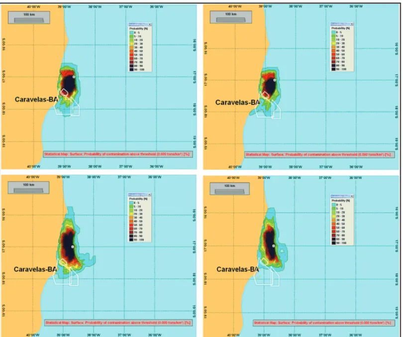
Figures 4 to 7 show the probabilistic simulations of oil spills oc-curring at blocks BM-CUM-1, BM-CUM-2, J-M-259 and ES-M-418, respectively. Each map in these figures displays probability contours which were computed from 80 deterministic simulati-ons. The austral summer simulations are shown in top panels of all figures, whereas the austral winter simulations are shown in the bottom panels. Conversely, the simulations that have considered the tides are shown in the left hand panels and the ones without the tidal currents in right hand panels. In our analysis, we care for the “APA Ponta das Baleias” and for the Buffer Zones 1 and 2

(the polygons contoured by white lines in all figures). The Buffer Zones are zones of no oil activity determined by the Federal Ins-titute of Environmental Protection (IBAMA) around the Abrolhos Reefs and the APA is a protected National Park. These areas are protected by law against oil activities.

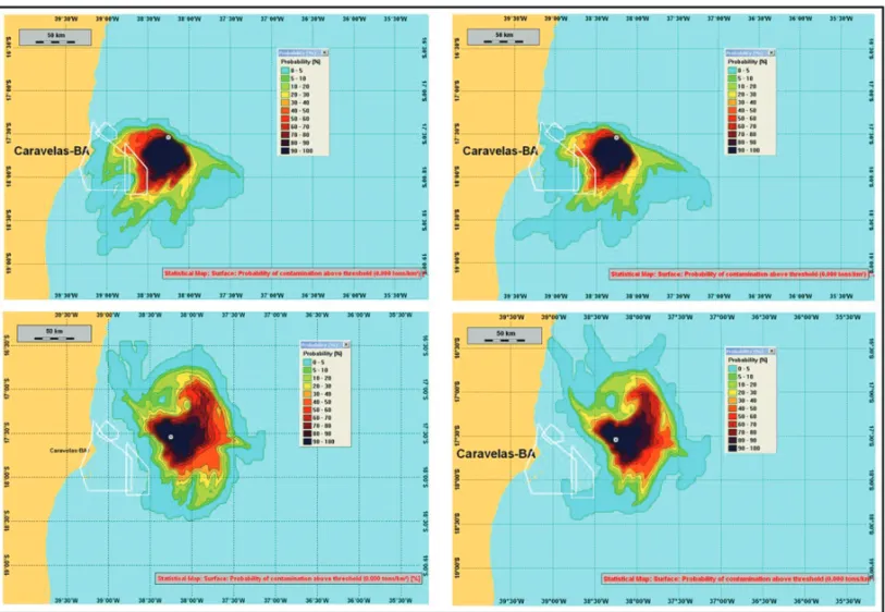
The most evident result, that is noticeable in all four figures, is the dominance of southward oil transportation during the sum-mer period and a very different pattern in the winter, when the oil was transported both northward and southward. The scenarios described above are a consequence of the seasonal changes in wind stress, with northeast winds dominating the whole summer period and strong wind reversals occurring during the winter, due to a higher frequency of atmospheric cold fronts. This is a pattern that is very evident in the simulations of oil block BM-CUM-1 (Fig. 4), where the summer spills show most of their contents (probability higher than 50%) being transported southwestwards, which is exactly toward the “APA Ponta das Baleias” (Fig. 4, top panels). However, the probability of summer spills reaching the APA and Buffer Zone 1 is higher in the presence of the tides (left hand top panel) than without the tides (right hand top panel). Probability contours as high as 80% and 90% reach the Preser-vation Areas (APA and Buffer Zones). During the winter (Fig. 4, bottom panels) the oil spreads along the shelf break, both north-wards and southnorth-wards, and again the spreading is higher in the presence of the tides (Fig. 4, left hand bottom panel) and so is the probability of the oil spills reaching the APA and the Buffer Zones. In the simulations of block BM-CUM-2, which is located southward from BM-CUM-1 and in areas where the BC main axis is directed southeastward (offshore), the oil spreading patterns are much different than in the former. The summer spills (Fig. 5, top panels), also have a tendency for southward spreading but with higher cross-shelf spreading than the spills of block BM-CUM-1. Although the area of the summer spills is larger in the absence of the tides (Fig. 5, top right hand panel), the probabi-lity of reaching the Protected areas is higher in the presence of the tides (see the probability contours in Figure 5, top left hand panel). The winter spills (Fig. 5, bottom panels) show very simi-lar patterns in the presence (left hand panel) and absence of the tides (right hand panel), although the area of the spill is larger in the simulation that considers the tides. An anti-cyclone circula-tion pattern caused the oil spill to drift offshore, toward deeper waters and then northward.

The simulations of block J-M-259, the northernmost block, show the most significant differences between the scenarios ob-tained in the presence and in the absence of the tides, especially during the summer period (Fig. 6, top panels). The summer spill

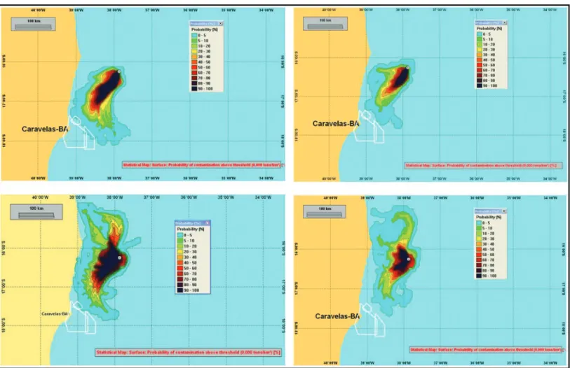
Figure 4 – Maps of probability of surface oil presence for BM-CUM-1 spills, resulting from spillage of 192 m3.day-1occurring without contingency during 30 days. Summer period simulations are presented on the top panels and winter period simulations on the lower panels. Simulations carried out with the tides are presented on the left hand panels and simulations without the tides on the right hand panels. The white line polygons are the Abrolhos Park Buffer Zones (two smaller polygons) and the Preservation Area Ponta das Baleias (larger polygon) and the location of spill is indicated by circumscribed x. Within the box in the bottom right corner one reads: “Statistical Map: Surface: Probability of contamination above threshold (0.000 tons/km2) [%]”.

is much more elongated in the presence of the tidal currents than in the absence of them. The winter spills (Fig. 6, bottom panels) show very similar patterns in both scenarios (with and without the tides). Although the probability of oil spills reaching the pro-tection areas are very low in both seasons, they only reach the APA and Buffer Zone 1 in the simulations that contain tidal va-riability. The spills for the simulations in the block ES-M-418 (Fig. 7) never reach the Protected areas and the spreading pat-terns obtained in the presence and in the absence of the tides are very similar (spill areas are slightly larger in the presence of the tides). This implies that the tidal currents are not a dominant pro-cess in this part of the domain.

A summary of all simulation results are presented in Tables 3 (summer) and 4 (winter). In these tables, we present informa-tion for each block, on three aspects of oil spills: the probability of it occurrence, the tonnage per area and the arrival time. We chose two control areas to present this information, one located to the left hand side of the spill location and another to the right hand side. In each of these control areas, we found the maximum probability of all 80 simulations, the maximum tonnage and mi-nimum arrival time. The arrival time is the time taken by the oil to arrive at the control areas.

We then have six columns for each block. In the first two columns we present the information concerning the left and the

Figure 5 – Maps of probability of surface oil presence for BM-CUM-2 spills, resulting from spillage of 192 m3.day–1occurring without contingency during 30 days. Summer period simulations are presented on the top panels and winter period simulations on the lower panels. Simulations carried out with the tides are presented on the left hand panels and simulations without the tides on the right hand panels. The white line polygons are the Abrolhos Park Buffer Zones (two smaller polygons) and the Preservation Area Ponta das Baleias (larger polygon) and the location of spill is indicated by circumscribed x. Within the box in the bottom right corner one reads: “Statistical Map: Surface: Probability of contamination above threshold (0.000 tons/km2) [%]”.

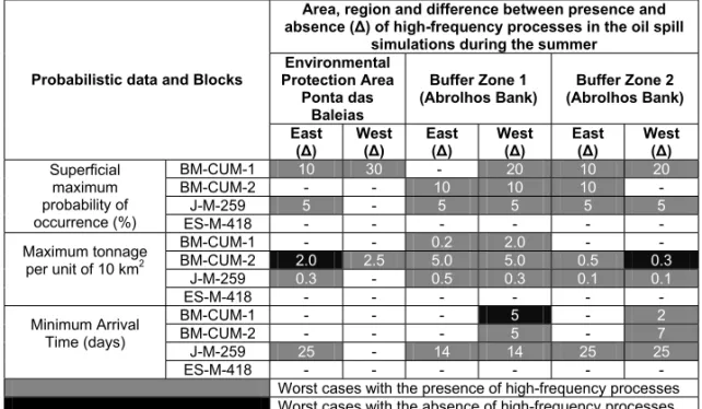
right hand side control areas of the APA, the third and fourth columns present the information concerning the Buffer Zone 1 and fifth and sixth columns refers to Buffer Zone 2, respectively. In each cell of each table we computed the difference between the information obtained in the simulations which have consi-dered the tides and the simulations which do not consider the tides. The cells that present the worst scenario in presence of the tides were painted in blue. Conversely, the cells with the worst scenario in the absence of the tides were painted in black. In a few words, the cells painted in blue show the negative results obtained when the tides were considered as one of the forcing mechanisms of the oil simulations.

The summer period simulations (Tab. 3) show that the worst scenarios occurred almost in all cases when the tides were considered. The worst cases were obtained in blocks BM-CUM-1, BM-CUM-2 and J-M-259. The probability of occurrence was 30% higher in the presence of the tides in the APA area

and 20% higher in the Buffer Zone 1. The winter period table (Tab. 4) show results which are in agreement with the informa-tion presented in Figures 4 to 7, where we see the worst scenario in block BM-CUM-1 in the presence of the tides, while the worst scenario in block BM-CUM-2 occurred in the absence of the tides. DISCUSSION AND CONCLUSIONS

Our results show very distinct scenarios for the winter and sum-mer periods during the year of 1989 (which was considered as a proxy to represent the seasonal variability) and for simu-lations with and without the tides. During the summer, the oil was transported southwestward in all cases, showing very lit-tle or nearly zero northward spreading. This was a consequence of the combined effects of the winds stress and the BC trans-port. The summer is the season when the area is under the in-fluence of the strongest northeast winds and when the BC shows

Figure 6 – Maps of probability of surface oil presence for J-M-259 spills, resulting from spillage of 192 m3.day–1occurring without contingency during 30 days. Summer period simulations are presented on the top panels and winter period simulations on the lower panels. Simulations carried out with the tides are presented on the left hand panels and simulations without the tides on the right hand panels. The white line polygons are the Abrolhos Park Buffer Zones (two smaller polygons) and the Preservation Area Ponta das Baleias (larger polygon) and the location of spill is indicated by circumscribed x. Within the box in the bottom right corner one reads: “Statistical Map: Surface: Probability of contamination above threshold (0.000 tons/km2) [%]”.

its highest poleward transport. As a result, little northward oil spreading was observed. Conversely, the winter simulations show northward oil transportation as intense as the southward transport and the area of the oil spill is nearly equal both northward and southward from the location of the spillage. This was also a con-sequence of the combined effects of the winds stress and the BC transport. During the winter, the wind reversals associated with the atmospheric frontal systems occur simultaneously with the weakest BC poleward transport, allowing the oil to be transpor-ted both northward and southward.

Another significant difference found between the winter and the summer simulations is the occurrence of instabilities and mesoscale features associated with the BC. The current shows reduced velocities and associated transport during the winter pe-riod, which result in a smaller contribution of the current baro-tropic mode, which is of greater contribution of instabilities and eddies. During the summer period, the Ilheus Eddy, the Royal Charlotte Eddy and the Abrolhos Eddy are intensified (Soutelino,

2008) and their contribution to offshore oil spreading is noticea-ble in Figures 5, 6, 7, and 8, specially in simulations of BM-CUM-2 block (Fig. 6).

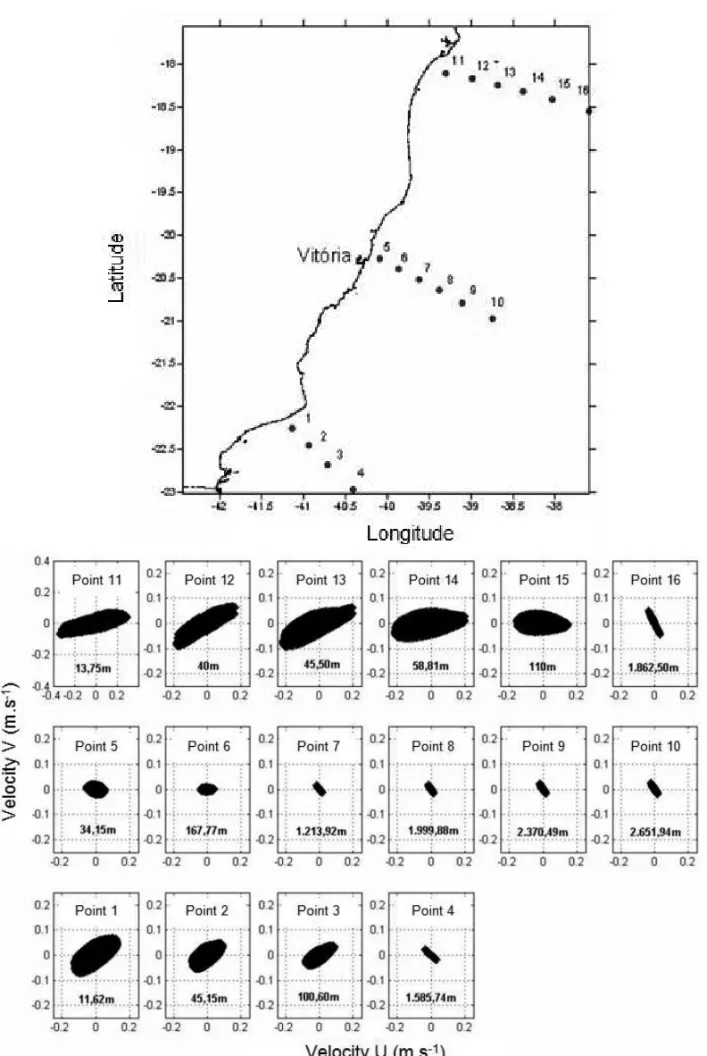
However, our most significant results are concerned to the effect of the tides within these wind-driven scenarios. The direc-tion of tidal currents is evident in Figure 8, where we present the tidal ellipses in the study domain. In this figure we reproduce the results obtained by Lemos (2006) who conducted numerical experiments with Princeton Ocean Model (POM). The model was implemented with a combination of radiational condition from Or-lanski (1976) and Flather (1986) in the boundary condition and seven tidal harmonic components (M2, S2, N2, K2, K1, O1, Q1)

from the global model FES95.2. The strongest currents occurred in the northern part of domain, where the ellipses are oriented in the NE-SW direction near the coast, changing to E-W direction offshore. In the southern part the currents are lighter, according mainly to the narrowing continental shelf, and the ellipses have the same orientation of the northern ellipses. In the southern

do-Table 3 – Comparative results of 80 probabilistic simulations with and without application of high-frequency filter for removal of

supra-inertial processes in scenarios of spill of 192 m3.day–1of degree API intermediate oil for 30 days during the summer in blocks BM-CUM-1, BM-CUM-2, J-M-259 and ES-M-418. The absence of data indicates that the values for the two oils are alike.

BM-CUM-1 10 30 -- 20 10 20 BM-CUM-2 - - 10 10 10 -J-M-259 5 - 5 5 5 5 Superficial maximum probability of occurrence (%) ES-M-418 - - - -BM-CUM-1 - - 0.2 2.0 - - BM-CUM-2 2.0 2.5 5.0 5.0 0.5 0.3 J-M-259 0.3 - 0.5 0.3 0.1 0.1 Maximum tonnage per unit of 10 km2 ES-M-418 - - - - BM-CUM-1 - - - 5 - 2 BM-CUM-2 - - - 5 - 7 J-M-259 25 - 14 14 25 25 Minimum Arrival Time (days) ES-M-418 - - - -

Worst cases with the presence of high-frequency processes Worst cases with the absence of high-frequency processes

Table 4 – Comparative results of 80 probability simulations with and without application of high-frequency filter for removal of

supra-inertial processes in scenarios of spill of 192 m3_.day–1_{of degree API intermediate oil for 30 days during the winter in blocks} BM-CUM-1, BM-CUM-2, J-M-259 and ES-M-418. The absence of data indicates that the values for the two oils are alike.

BM-CUM-1 25 15 5 25 10 20 BM-CUM-2 5 - - 5 - - J-M-259 - - - - 5 -Superficial maximum probability of occurrence (%) ES-M-418 - - - - BM-CUM-1 2.0 2.0 3.0 2.0 2.0 2.0 BM-CUM-2 0.1 - - 1.0 - - J-M-259 - - - - 0.3 -Maximum tonnage per unit of 10 km2 ES-M-418 - - - - BM-CUM-1 10 10 10 10 2 3 BM-CUM-2 25 - - 25 - - J-M-259 - - - - 25 -Minimum Arrival Time (days) ES-M-418 - - - -

Worst cases with the presence of supra-inertial processes Worst cases with the absence of supra-inertial processes

main the effects of the tidal on oil spreading were less expres-sive, showing lowest differences between simulations with and without tidal, mainly the simulations in the block ES-M-418.

The most evident cases of the effect of the tides were obser-ved in the J-M-259 simulations. The areas of the J-M-259 spills

are significantly larger in the presence of the tides than without them, especially during the summer simulation. The oil spills re-sulting from the J-M-259 spillages never reached the protected areas in the simulations carried out without the tides, while con-tamination of these areas (“APA Ponta das Baleias” and Abrolhos

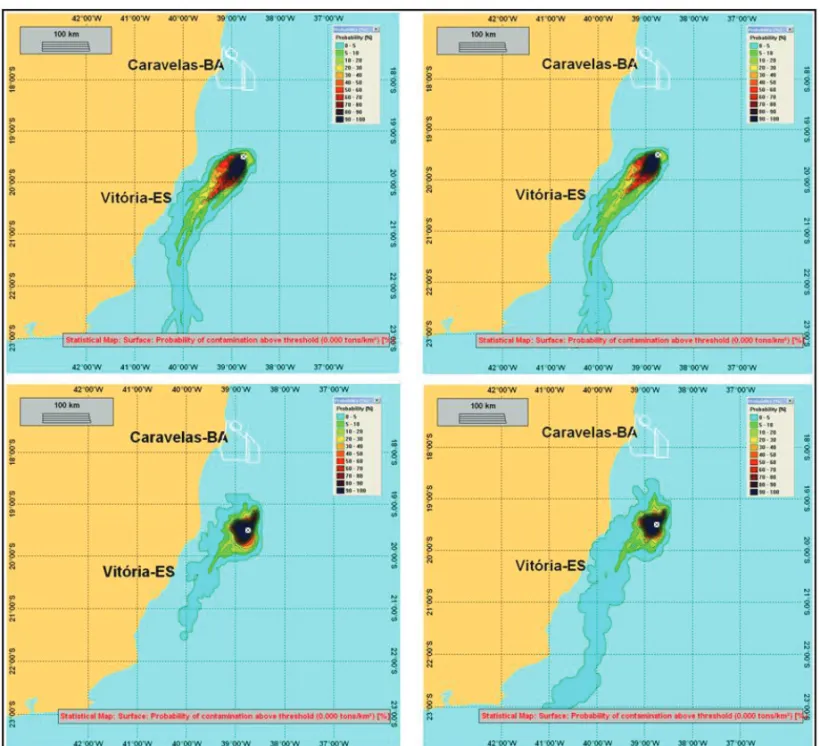
Figure 7 – Maps of probability of surface oil presence for ES-M-418 spills, resulting from spillage of 192 m3.day–1occurring without contingency during 30 days. Summer period simulations are presented on the top panels and winter period simulations on the lower panels. Simulations carried out with the tides are presented on the left hand panels and simulations without the tides on the right hand panels. The white line polygons are the Abrolhos Park Buffer Zones (two smaller polygons) and the Preservation Area Ponta das Baleias (larger polygon) and the location of spill is indicated by circumscribed x. Within the box in the bottom right corner one reads: “Statistical Map: Surface: Probability of contamination above threshold (0.000 tons/km2) [%]”.

Bank) has occurred both during the winter and the summer simu-lations which were conducted with the tides. The J-M-259 block is located out of the continental shelf, on the slope, where the depth is 1179 m. The BC is the dominant feature on the slope, forcing oil transportation along the slope, inhibiting transport toward the shallow waters. The effect of the tides in these cases was to transport part of the oil toward shallow waters, where the wind stress is more effective. Once the oil reached the shallow

waters, the wind stress spread the oil more effectively, resulting in a thinner oil spill over a large surface area.

The BM-CUM-1 simulations showed the worst scenarios in the presence of the tides whereas the BM-CUM-2 simulations showed the worst scenarios in the absence of the tides. The BM-CUM-1 block is located to the north of the protection areas and the BM-CUM-2 is located to the east of the same areas. Without the tides, the BM-CUM-1 spills were transported by the BC toward

southeast, away from the protection areas. When the tides were considered the cross-shelf transport provided by the tidal currents spread part of the oil toward shallow waters and the oil ended up reaching the APA and the Buffer Zone 1. Conversely, the tidal currents produced the opposite effect on the BM-CUM-2 spills. Because this block is located to the east of the protection areas, the southwestward transport due to tidal currents spread the oil away from the protection areas, and the worst scenarios occurred when the tides were not considered as one of the forcing mecha-nisms. The ES-M-418 spills never reached the protection areas, with or without the tides.

We then conclude that the tides have strongly influenced the fate of the oil in most of our simulations, especially in blocks loca-ted in Cumuruxatiba (BM-CUM-1 and BM-CUM-2) and Jequiti-nhonha (J-M-259) basins. The tidal currents were more effective in the Abrolhos Bank, where the cross-shelf transport provided by the tidal currents resulted in higher probabilities of oil con-tamination of the protection areas due to BM-CUM-1 spill. The worst scenarios occurred in the summer simulations of blocks BM-CUM-1, BM-CUM-2 and J-M-259, specially because these blocks are closer to the protection areas.

ACKNOWLEDGEMENTS

We acknowledge the financial support obtained from the ANP Human Resources Program (PRH 27), which provided Mr. Lemos MSc scholarship, and the Associac¸˜ao ATLANTIS (www.atlantis.org.br), which contributed with computer logistic and funding for participation in Workshops and PRH events. Dr. Cirano was supported by CNPq research Grant. We also acknowl-edge the logistic support provided by the Universidade Federal do Rio Grande and the Universidade Federal do Esp´ırito Santo. REFERENCES

AAMO OM, REED M & DOWNING K. 1997. Oil spill contingency and response (OSCAR) model system: Sensitivity studies. In: 1997 Interna-tional Oil Spill Conference, 22 pp.

BLUMBERG AF & MELLOR GL. 1987. A description of a three-dimen-sional coastal ocean circulation model. In: HEAPS N (Ed.). Three-di-mensional ocean models. Am. Geophys. Union, 16 pp.

BOEHM PD. 1987. Transport and transformation processes regarding hydrocarbon and metal pollutants in offshore sedimentary environments. In: BOESCH DF & RABALAIS NN (Ed.). Long-term environmental ef-fects of offshore oil and gas development. Appl. Sci., Elsevier, 233-287, London & New York.

CAMPOS EJD. 1995. Estudos da circulac¸˜ao oceˆanica no atlˆantico

tropi-cal e regi˜ao oeste do atlˆantico subtropitropi-cal sul. Tese de Livre Docˆencia. Universidade de S˜ao Paulo, Instituto Oceanogr´afico, 114 pp.

CASTRO BM & MIRANDA LB. 1998. Physical oceanography of the western Atlantic continental shelf located between 4◦_{N and 34}◦_S

coastal segment (4◦_{). In: ROBINSON AR & BRINK KH (Org.). The Sea.}

209–251.

CIRANO M, MATA MM, CAMPOS EJD & DEIR ´O NFR. 2006. A circulac¸˜ao oceˆanica de larga-escala na regi˜ao oeste do Atlˆantico Sul com base no modelo de circulac¸˜ao global OCCAM. Revista Brasileira de Geof´ısica, 24(2): 209–230.

FINGAS M. 2001. The basics of oil spill cleanup. CRC Press LLC, vol. 2, 233 pp.

FLATHER RA. 1986. A tidal model of the northeast Pacific. Atmos. Ocean, 25: 22–25.

GAETA SA, LORENZZETTI JA, MIRANDA LB, SUSINI-RIBEIRO SMM, POMPEU M & ARAUJO CES. 1999. The Vit´oria Eddy and its relation to the phytoplankton biomass and primary productivity during the austral fall of 1995. Arch. Fish. Mar. Res., 47: 253–270.

KALNAY E, KANAMITSU M, KISTLER R, COLLINS W, DEAVEN D, GAN-DIN L, IREDELL M, SAHA S, WHITE G, WOOLLEN J, ZHU Y, CHELLIAH M, EBISUZAKI W, HIGGINS W, JANOWIAK J, MO KC, ROPELEWSKI C, WANG J, LEETMAA A, REYNOLDS R, JENNE R & JOSEPH D. 1996. The NCEP/NCAR 40-year reanalysis project. Bull. Amer. Meteor. Soc., 77: 437–471.

LE˜AO ZMAN. 1999. Abrolhos – O complexo recifal mais extenso do Atlˆantico Sul. In: SCHOBBENHAUS C, CAMPOS DA, QUEIROZ ET, WINGE M & BERBERT-BORN MLC (Eds.). Geological and Paleontolo-gical Sites of Brazil. DNPM/CPRM, SIGEP 90, 345–359.

LEMOS AT. 2006. Modelagem num´erica da mar´e barotr´opica na costa do Esp´ırito Santo. TCC, Universidade Federal do Esp´ırito Santo, 65 pp. LE PROVOST C, LYARD F, MOLINES JM, GENCO ML & RABILLOUD F. 1998. A hydrodynamic ocean tide model improved by assimilating a sa-tellite altimeter-derived data set. J. Geophys. Res., 103(C3): 5513–5529. LESSA GC & CIRANO M. 2006. On the circulation of a Coastal Chan-nel Within the Abrolhos Coral-Reef System – Southern Bahia (17◦₄₀0_S),

Brazil. J. Coastal Res., Sl 39: 450–453.

LESSA GC, TEIXEIRA CEP & CIRANO M. 2005. Trˆes Anos de Intenso Mo-nitoramento na Zona Costeira do Banco de Abrolhos: Existem indicac¸˜oes de Impacto da Dragagem nos Recifes de Coral?. In: II Congresso Brasi-leiro de Oceanografia, 2005, Vit´oria (ES). CD-ROM, 3 pp.

ORLANSKI I. 1976. A simple boundary condition for unbounded hyper-bolic flows. J. Comput. Phys., 21: 251–269.

REED M, AAMO OM & DALING PS. 1995. Quantitative analysis of alter-nate oil spill response strategies using OSCAR. Spill Sci. Technol. Bull. Elsevier, 2(1): 67–74.

REED M, JOHANSEN Ø, BRANDVIK PJ, DALING P, LEWIS A, FIOCCO R, MACKAY D & PRENTKI R. 1999. Oil spill modeling towards the close of the 20th_{century: Overview of the state of the art. Spill Sci. Technol. Bull.}

Elsevier, 5(1): 3–16.

REED M, DALING P, LEWIS A, DITLEVSEN MK, BRORS B, CLARK J & AURAND D. 2004. Modeling of dispersant application to oil spills in shallow coastal waters. Environ. Modell. Softw., 19: 681–690. RODRIGUES RR, ROTHSTEIN LM & WIMBUSH M. 2006. Seasonal Variability of the South Equatorial Current Bifurcation in the Atlantic Ocean: A Numerical Study. J. Phys. Oceanogr., 37: 16–30.

SCHMID C, SCH¨AFER H, ZENK W & PODEST´A G. 1995. The Vit´oria Eddy and its Relation to the Brazil Current. J. Phys. Oceanogr., 25(11): 2532–2546.

SCHMIDT ACK. 2004. Interac¸˜ao Margem Continental, v´ortices e jatos geof´ısicos. Tese de Doutorado, Instituto Oceanogr´afico. Universidade de S˜ao Paulo, 221 pp, S˜ao Paulo – SP.

SILVEIRA ICA, BROWN WS & FLIERL GR. 2000a. Dynamics of the North Brazil Current Retroflection Region from the WESTRAX Observations. J. Geophys. Res.-Oceans, 105(12): 28559–28584.

SILVEIRA ICA, SCHMIDT ACK, CAMPOS EJD, GODOI SS & IKEDA Y. 2000b. A Corrente do Brasil ao Largo do Sudeste Brasileiro. Rev. Bras. Oceanogr., 48(2): 171–183, S˜ao Paulo – SP.

SOARES SM. 2007. Ondas Inst´aveis de Correntes de Contorno Oeste ao Largo de Abrolhos. Dissertac¸˜ao de Mestrado – Instituto Oceanogr´afico da Universidade de S˜ao Paulo – IO/USP, 98 pp, S˜ao Paulo – SP. SOUTELINO RG. 2008. A Origem da Corrente do Brasil. Dissertac¸˜ao de Mestrado – Instituto Oceanogr´afico da Universidade de S˜ao Paulo – IO/USP, 120 pp, S˜ao Paulo – SP.

STRAMMA L & ENGLAND M. 1999. On the water masses and mean circulation of the South Atlantic Ocean. J. Geophys. Res., 104(C9): 20863–20883.

WEBB D, CUEVAS BA & COWARD AC. 1998. The first main run of the OCCAM global ocean model. Tech. Rep. 34, Southampton Oceano-graphy Centre, 43 pp.

ZEMBRUSCKI S. 1979. Geomorfologia da margem continental sul bra-sileira e das bacias oceˆanicas adjacentes. Petrobras, Cenpes, 129–177, Rio de Janeiro – RJ.

NOTES ABOUT THE AUTHORS

Angelo Teixeira Lemos is an oceanographer (UFES/2006) with a MSc in Physical, Chemical and Geological Oceanography at Federal University of Rio Grande

(FURG/2009) and currently in second year of PhD in Environmental Oceanography from UFES. His research is focused in numerical modeling of meso and large-scale hydrodynamics process and oil spill at sea.

Ivan Dias Soares is an Associated Lecturer at the Federal University of Rio Grande and a member of the border of directors of the Atlantis Association for

Science Development. Ivan got his PhD diploma at the Rosenstiel School of Marine and Atmospheric Science/University of Miami, in Physical Oceanography, in 2003 and is now conducting the LENOC (Laboratory for Numerical Experiments in Ocean Science), which main research fields are physical oceanography and numerical modeling of ocean processes.

Renato David Ghisolfi has got a BSc. degree in Chemical Engineering (FURG/1988) and Oceanology (FURG/1990) and MSc. degree in Remote Sensing (UFRGS/

1995). His Ph.D. is in Physical Oceanography awarded by the University of New South Wales, Sydney, Australia (2001). Since June 2004 he is working as a professor and a researcher at the Federal University of Esp´ırito Santo (UFES) with focus on Physical Oceanography. His research interest is mainly on numerical modelling, acting on the following topics: numerical modelling of ocean dynamics, oil dispersal and contingency plans, besides obtaining and analysingin situdata.

Mauro Cirano is an oceanographer (FURG/1991) with a MSc in Physical Oceanography at University of S˜ao Paulo (IO-USP/1995) and a Ph.D. in Physical

Oceanography at the University of New South Wales (UNSW), Sydney, Australia (2000). Since 2004, he has been working as an Associate Professor at the Federal University of Bahia (UFBA). His research interest is the study of the oceanic circulation, based on data analysis and numerical modeling, area where he has conducting research projects over the last 15 years, focusing on the meso and large-scale aspects of the circulation.