Sba Controle & Automação vol.13 número1

THE PERFORMANCE SURFACE IN NONLINEAR MEAN SQUARE

ESTIMATION: APPLICATION TO ACTIVE NOISE CONTROL

PROBLEMS WITH CORRELATED SIGNALS

M´

arcio H. Costa

Jos´

e C. M. Bermudez

bermudez@eel.ufsc.br

Neil J. Bershad

∗ _{Lab. de Engenharia Biom´edica, Escola de Engenharia, Universidade Cat´olica de Pelotas, Pelotas, RS, Brazil}

† _{Depto de Engenharia El´etrica, Universidade Federal de Santa Catarina, Florian´opolis, SC, Brazil}

‡ _{Department of Electrical and Computer Engineering, University of California, Irvine, CA, USA}

ABSTRACT

This paper investigates the properties of the perfor-mance surface for the problem of nonlinear mean-square estimation of a random sequence. The problem stud-ied has direct application to the study of active noise control (ANC) systems when the transducers are driven into a nonlinear behavior. A deterministic expression is derived for the mean-square error (MSE) surface as a function of the system’s degree of nonlinearity for Gaus-sian correlated input signals. It is shown how the pres-ence of the nonlinearity deforms the MSE surface. It is demonstrated that the surface is unimodal, and the ex-pression for the optimum weight vector is determined. The new results are then used to quantify the behav-ior of ANC systems employing the LMS adaptive algo-rithm. Important algorithm properties are derived from this study. Examples are presented which verify the an-alytical models derived.

KEYWORDS: active noise control, adaptive filters, adap-tive algorithms, nonlinear systems, estimation theory.

Artigo submetido em 20/11/00

1a. Revis˜ao em 07/01/01; 2a. Revis˜ao em 01/11/01

Aceito sob recomenda¸c˜ao do Ed. Cons. Prof. Dr. Jos´e Roberto Castilho Piqueira

RESUMO

Este artigo investiga as propriedades da superf´ıcie de desempenho para o problema de estima¸c˜ao m´edia qua-dr´atica n˜ao-linear de uma seq¨uˆencia aleat´oria. Os re-sultados obtidos possuem aplica¸c˜ao direta no estudo de sistemas de controle ativo de ru´ıdo (CAR) quando os

transdutores possuem um comportamento n˜ao-linear. ´E

desenvolvida uma express˜ao determin´ıstica para a su-perf´ıcie do erro m´edio quadr´atico em fun¸c˜ao do grau de

n˜ao-linearidade, supondo-se sinais de entrada

gaussia-nos correlacionados. Atrav´es deste resultado ´e determi-nado o vetor de coeficientes ´otimo, demonstrada a uni-modalidade da superf´ıcie de erro e a maneira pela qual a

presen¸ca da n˜ao-linearidade a deforma. A partir disto,

os resultados obtidos s˜ao utilizados para quantificar o

comportamento de sistemas CAR que empregam o al-goritmo adaptativo LMS. Como resultado, importantes

propriedades do algoritmo s˜ao verificadas. Finalizando,

simula¸c˜oes comprovam a validade dos modelos anal´ıticos desenvolvidos.

1

INTRODUCTION

Mean square estimation plays a crucial role in many problems of adaptive control (Ren and Kumar, 1992) and adaptive signal processing (Haykin, 1996). There-fore, the question of how to design adaptive estima-tion systems for optimized behavior has met consider-able interest. Optimal system designs require detailed knowledge about the theoretical problem and about the adaptive algorithm performance in solving that prob-lem. Such knowledge is obtained through analysis of the system behavior and derivation of analytical models that can accurately predict this behavior.

Analyses of practical systems’ behavior always rely on restrictive assumptions to make the mathematical task feasible. The resulting analytical model is applicable to situations in which the effects of the neglected nonide-alities are not significant.

Active noise and vibration control (ANC) is a technique

extensively used by the control (Angevine, 1995; F¨uller

and Flotow, 1995) and signal processing (Kuo and Mor-gan, 1996; Hansen, 1997) communities. It consists of cancelling sound or vibrational waves through destruc-tive interference. A practical example is the noise reduc-tion in ventilareduc-tion ducts (Massaraniet alii,1990; Os´orio

and N´obrega, 1995).

Adaptive linear control techniques have been largely ap-plied in ANC (Kuo and Morgan, 1996). However, con-siderable nonlinear effects from overdriven loudspeakers, piezoelectric transducers or power amplifiers in the sec-ondary path (the path leading from the adaptive filter output to the cancellation point) have been reported in actual ANC systems. In addition, correlated input sig-nals are very common in ANC applications (Kuo and Morgan, 1996; Hansen, 1997).

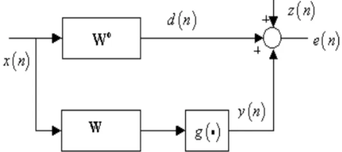
Fig. 1 shows the block diagram of an ANC system in-fluenced by a nonlinearity in the secondary path. The

block g(·) is a saturation nonlinearity. It represents

the composed nonlinear effects in that path (Costa et

alii, 1999). The design problem usually consists of

de-termining the optimum control weight vector W _that

minimizes the mean square error (MSE) at the system

output (Os´orio and N´obrega, 1995). In this case,

min-imization of the MSE defines a nonlinear mean square

estimation problem. The random signal d(n) is

esti-mated by a nonlinear function of the reference signal x(n) (Papoulis, 1991 – section 7-5).

Although ANC system nonlinearities are quite common, very little has been reported in the literature on their ef-fects on the MSE surface. Therefore, very little is known

Figure 1: Block diagram of the system analyzed.

about the behavior of adaptive algorithms used to can-cel undesirable noise under this constraint. A recent

paper (Costa et alii, 1999) has studied the statistical

behavior of the system in Fig. 1 when the filter

coeffi-cient vectorW_{is adjusted using the Least Mean Square}

(LMS) adaptive algorithm. The analysis presented in

Costaet alii(1999) determined analytical models for the

mean weight and the MSE behaviors for slow adaptation and white input signals. Very accurate estimates of the transient and steady-state algorithm behavior were ob-tained. However, this analysis does not provide all the necessary design information if the MSE performance surface properties are unknown. The knowledge of such properties allows the designer to determine the algo-rithm behavior for a given degree of nonlinearity, as compared to the optimum. In addition, the MSE surface properties are necessary for a meaningful performance comparison among different adaptive algorithms.

An initial investigation Costa et alii (2000) has

deter-mined the MSE surface properties for white Gaussian in-puts. Though these results lead to important insights on the characteristics of the nonlinear estimation problem, they do not provide accurate information for the impor-tant case of correlated input signals (Kuo and Morgan, 1996; Hansen, 1997).

This paper extends the analysis of (Costaet alii, 2000)

to determine the MSE surface property for systems with correlated input signals. A deterministic expression is derived for the MSE surface as a function of the system’s degree of nonlinearity. It is shown how the presence of the nonlinearity deforms the MSE surface. The surface is shown to remain unimodal for any degree of nonlin-earity. The optimum weight vector and the minimum MSE are determined.

predictable loss in performance becomes feasible.

Next, the particular but important case of the LMS algorithm is studied. The MSE surface properties are used to provide new insights on the behavior of the al-gorithm when applied to ANC systems. New results are presented for the LMS algorithm behavior with corre-lated input signals. The MSE misadjustment and the converged weight misalignment are determined as func-tions of the system’s degree of nonlinearity. It is verified that the converged mean weight vector for the LMS is a scaled version of the optimum weight vector.

2

ANALYSIS OF THE MSE SURFACE

The block diagram in Fig. 1 shows the nonlinear mean

square estimation problem studied. This diagram is

representative of an ANC system with loudspeakers or piezoelectric transducers driven into nonlinear operation (Bernhardet alii, 1997).

Wo ₌

wo

0 wo1 . . . woN−1

T

is the vector of the impulse response samples of a linear system (plant).

W₌

w0 w1 . . . wN−1

T

is the transversal FIR linear controller weight vector. d(n) is the signal to be estimated (primary signal). x(n) is the reference signal which is assumed stationary, zero-mean and Gaussian. X₍n) =

x(n) x(n₋1) . . . x(n₋N+ 1) T

is

the observed data vector andRXX=E

X_(n)XT_(n)

is the reference input correlation matrix. z(n) is the

measurement noise, assumed stationary, white,

gaus-sian, zero-mean, with varianceσ2

zand uncorrelated with

any other signal. y(n) is the control signal, ande(n) is the error signal to be minimized in the MSE sense. The nonlinearity is modeled by the scaled error function:

g(y) =

y

0

e− z 2

2σ2_{dz (1)}

Note that lim

σ→∞g(y) =yand limσ→0g(y) =σ

π

2 sgn (y).

Hence,g(y) properly scaled can range between a linear

device and a hard limiter by varyingσ.

2.1

MSE Performance Surface

The error signal in Fig. 1 is given by:

e(n) =d(n) +z(n)−g_WT_X(n)

=WoTX_{(n) +z(n)−gW}T_X(n)

(2)

Squaring (2) and taking the expected value yields:

Ee2(n)

=WoT_EX_(n)XT_(n)Wo

+E

z2(n)

+ 2WoTE_{z(n)X₍n)} −2E

g_WT_X(n)

z(n)

−2WoT_E

g_WT_X(n)X

(n)

+E

g2

WTX₍n)

(3)

The first four expectations are easily evaluated

us-ing the statistical properties of x(n) and z(n):

E

X₍n)XT₍n)

= RXX; E

z2_(n)

= σ2

z;

E{z(n)X_(n)}=0_andE

g_WTX

(n)

z(n)

= 0.

Since x(n) is zero-mean Gaussian and W _{is constant,}

the last two terms in (3) include expectations of non-linear functions of zero-mean Gaussian variables. The fifth expectation can be obtained from Shynk and

Ber-shad (1991) for b1 = 0, σq = σ, c = 1/σ and σ2y =

WT_{RXXW. Thus,}

EgWTX_(n) X_(n)= 1

1

σ2W

T_R

XXW+ 1

R_XXW

(4)

The last expectation can be obtained from (Bershad

et alii, 1993 - Appendix) for αf = 1, b1(n) = 1and

b=WT_RxxWas

E

g2_WT_X(n)

=σ2 arcsin

_WT_R

XXW

WTRXX W+σ2

(5)

Combining the above results into (3) yields an analytical expression for the MSE surface:

ξ=E

e2(n)

=WoTRXXW

o

+σ2_z

− 2

1

σ2WTRXXW+ 1

WoTRXXW

+σ2arcsin

_WT_R

XXW

WT_RXXW+σ2

(6)

The system’s degree of nonlinearity is defined as

η2= π 2

σ2_d max{σ2

y}

(7)

This parameter relates the power of d(n) to the

maxi-mum power at the output of the nonlinearity. It can be

easily shown by taking the limit of (1) asy → ∞that

max{σ_y2}= π

2σ

2_{. Thus,}

η2= 1 σ2W

o_T

RXXW o

For the linear case, σ→ ∞andη2→0.

Fig. 5 presents examples of the MSE surface for

differ-ent degrees of nonlinearityη2_{. Notice that the surface}

deforms asη2 _{increases. Regions of slower convergence}

(small gradient) appear as η2 _{increases. However, it}

remains unimodal for any degree of nonlinearity. This important result will be demonstrated in the next sub-section. Note that the MSE (6) is not minimized by

W₌Wo

unless η2= 0 (linear case).

2.2

Stationary Points

Differentiating (6) with respect to the weight vector and equating it to zero yields an expression for the minima

˜

W_{of the MSE surface. Thus,}

∂ ∂W   2 1

σ2WTRXXW+ 1

WoTRXXW  

W₌W˜

=

=σ2 ∂

∂W

arcsin

_WT_RXXW

WTRXXW+σ2

_W

=W˜

(9)

Evaluating the derivatives in (9) and setting W ₌W˜

yields:

Wo

+_σ12

Wo_W˜T

−WW˜ oT RXXW˜

1

σ2W˜TRXXW˜ + 1

1/2 = = ˜ W 2

σ2W˜TRXXW˜ + 1

1/2 (10)

Equation (10) can be written as:

˜

W₌

1 + 1

σ2W˜TRXXW˜

1

σ2W

o_TR

XXW˜ +(

1

σ2W˜

T_R

XXW˜+1)

1/2

(2

σ2W˜

T_R

XXW˜+1)

1/2

Wo ₍₁₁₎

Note that all terms in the fraction multiplyingWo

in (11) are real nonegative scalars. Thus, the optimum weight vectorW˜ _{is a scaled versionc}Wo

ofWo

,c∈R+.

SubstitutingcWo

for_W˜ _{and using (8) in (11) yields:}

Wo

(c2_η2_{+ 1)}1/2 =

cWo

(2c2_η2_{+ 1)}1/2 (12)

Note thatc _∈R+. For givenWo

and η2, the constant

cmust be a solution of:

c4+

1 η2 −2

c2− 1

η2 = 0 (13)

Equation (13) yields four solutions:

c1,2,3,4=±

1−₂1_η2 ±

1

4η4 + 1 (14)

Because c must be real and positive, only the positive

sign is acceptable outside the square roots. In addition,

it is well known thatc= 1 is the only optimal solution

(the Wiener solution) forη2 _{→0 (g(y) =y, linear case).} This eliminates the possibility of the minus sign within the square root (the minus sign would lead to a complex

value forcasη2→0). Thus, the only allowable solution

for (13) is:

c=

1−₂1_η2 +

1

4η4 + 1 (15)

The minimum of the MSE surface is then:

˜

W₌

1−₂1_η2+

1

4η4 + 1·W

o

(16)

Fig. 2 shows the effect of the nonlinearity on the posi-tioning of the optimum weight vector in the direction of Wo

.

Using (16) in (6) yields an expression for the minimum of the MSE performance surface:

ξM IN =σz2+

1− √ 2c

c2_η2₊₁ +_η12 arcsin

c2η2 c2_η2₊₁ W

oT_R

XXWo

(17)

Fig. 3 shows the excess MSE (ξex=ξM IN−σz2) caused

by the nonlinearity, relative to the linear case, for the

normalized caseWoTRxxW

o

= 1. Eq. (17) determines the best performance that can possibly be expected from any adaptive algorithm used to solve the nonlinear esti-mation problem depicted in Fig. 1.

3

APPLICATION TO ANC SYSTEMS

Several control techniques can be used to optimize the weight vector in the system of Fig. 1. One of them is the adaptive system depicted in Fig. 4. Thus, the results of Section 2 can be used to quantify the performance of the LMS algorithm in a nonlinear ANC system. A similar approach can be used with other solutions to the ANC

problem (Massarani et alii,1990; Os´orio and N´obrega,

1995).

Analytical expressions have been derived in Costaet alii

LMS algorithm with white Gaussian inputs and slow adaptation. These expressions can be expanded to the correlated input signal case as:

W_{∞ = lim}

n→∞E{

W_(n)}= 1

1 -η2W

o

(18)

ξ∞= lim

n→∞ξ(n) =

WoTRXXW o

₁

η2arcsen

η2

−1

+σ2_z (19)

Note that the converged mean LMS weight vectorW_∞

is also a scaled version of the optimum solutionWo

for the linear case. Using (16) and (18) it is easy to show that:

W_∞=

2η2

(1−η2₎

1 + 4η4_−2η4_{+ 3η}2₋₁

1/2

˜

W_=β W˜ ₍₂₀₎

0 2 4 6 8 10

1 1.05 1.1 1.15 1.2 1.25 1.3 1.35 1.4

Degree of nonlinearity

c

Figure 2: Effect of the nonlinearity on the positioning of the optimum weight vector versus the degree of non-linearity.

Equation (20) shows that the LMS algorithm produces

a biased estimate of the optimum weight vectorW˜_{. The}

multiplicative biasβin (20) is a function of the system’s

degree of nonlinearity.

Using (17) and (19), the LMS excess MSE can be deter-mined:

ξ=ξ∞ −ξM IN

=

1 η2

arcsin

η2

−arcsin

c2_η2

c2_η2_{+ 1}

+ 2c

c2_η2_{+ 1}−2

WoTRXXW o

(21)

0 2 4 6 8 10

-50 -45 -40 -35 -30 -25 -20 -15 -10 -5 0

Degree of nonlinearity

Ex

c

e

s

s

M

SE

(d

B)

Figure 3: Excess MSE versus the degree of nonlinearity.

The misadjustment can be obtained normalizing (21):

M = ξexLM S ξM IN

(22)

Note that (20), (21) and (22) hold only forη2<1. The

mean weight of the LMS algorithm does not converge for η2_{1 (Costaet alii, 1999).}

Figure 4: Block diagram of the adaptive system.

3.1

Numerical Example

This section presents simple examples to illustrate the

application of the analytical results. Consider the

system in Fig. 1 with Wo _{= 0}.707 0.707 T

, WoTWo _{= 1,} σ2

z = 10−6 and a unit-variance

corre-lated input signal. The eigenvalue spread (λmax/λmin)

ofRXX is equal to 24.

Fig. 5 shows the MSE surface for three different de-grees of nonlinearity. Note the increasing deformation (with increasing asymmetry) of the MSE surface with

increasing η2_{. The LMS algorithm does not converge}

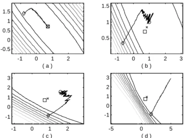
Assuming Fig. 4 with the same parameters described as above, Fig. 6 shows the MSE surface contours and the

LMS weight trajectories for random initialization,µ =

0.01 and four different degrees of nonlinearity. Vectors

Wo

and W˜ _{are also shown. Notice that in all cases}

Wo

,W˜ _{and the converged LMS weight vector}W_{∞ are}

aligned with the point (0,0) (the LMS weights converge asymptotically to this line in plot (d)). This behavior is in accordance with equations (16) and (20). Figs. 6a-6c

show the weights convergence for η2 _{< 1. For a small}

η2_{(Fig. 6a) the converged weights closely approach the}

minimum of the MSE surface (which also tends toWo_).

Fig. 6d show the divergence of the LMS algorithm for η2_>1.

Figure 5: MSE surfaces: (a)η2 _{= 10}−5_{; (b)η}2 _{= 0.01,} (c)η2_{= 2.}

-1 0 1 2

-0.5 0 0.5 1 1.5

( a )

-1 0 1 2 3

0.5 1 1.5

( b )

-1 0 1 2

-1 0 1 2 3

( c )

-5 0 5

-1 0 1 2 3

( d )

Figure 6: MSE contours and weight trajectories. ♦:

Wo_{; Υ:} W_{∞; ×:} W˜_{; ♦: LMS initialization; Ragged}

curves: weight trajectories; Continuous curves: MSE surface. (a)η2 = 10−5_{; (b) η}2 _{= 0.5; (c) η}2 _{= 0.8 and} (d)η2 = 2.

Figs. 7 and 8 show the weight bias β (Eq. (20)) and

the MSE misadjustment as a function ofη2. Asη2→0

(linear case), β → 1. When η2 → 1, β increases very

fast and finally grows without bound.

0 0.05 0.1 0.15 0.2 0.25 0.3 0.35 0.4 0.45 0.5 1

1.02 1.04 1.06 1.08 1.1 1.12 1.14 1.16 1.18 1.2

Degree of nonlinearity

W

ei

gh

t

bi

as

Figure 7: Weight biasβ caused by the LMS algorithm

as a function ofη2.

Figs. 9 and 10 show the simulated MSE and the be-havior of the first coefficient for a system with 30

co-efficients, µ = 0.01, σ_z2 = 10−6_{, 500 runs and R}

XX

0 0.1 0.2 0.3 0.4 0.5 0

0.05 0.1 0.15 0.2 0.25 0.3 0.35 0.4

Degree of nonlinearity

M

is

a

dj

us

tm

en

t

Figure 8: Misadjustment caused by the LMS algorithm as a function ofη2.

The distance between each curve in steady-state and the corresponding minimum confirm the difference between (17) and (19). Fig. 10 shows the behavior of the first adaptive weight (similar behavior was verified for all co-efficients). Again, the optimum solutions (Eq. (16)) are shown as lines of circles. Mismatches between steady-state weight behavior and optimum weight confirm the weight mismatch derived in Eq. (20).

0 1000 2000 3000 4000 5000 6000 7000 -60

-50 -40 -30 -20 -10 0 10

iterations

MS

E

(c)

(b)

(a)

Figure 9: Simulated mean square error (ragged curve) and the minimum of the performance surface (o o o). (a)η2_{= 0.0005; (b)η}2_{= 0.05; (c)η}2_{= 0.5.}

Two important results can be inferred from Fig. 9 and 10: (1) the LMS algorithm cannot achieve the minimum of the performance surface, generating a biased solution (multiplicative bias); (2) if the real system is incorrectly modeled as a linear system, the effect of the nonlinearity can cause a significant overestimation of the noise can-cellation capabilities of any adaptive algorithm based on mean square estimation.

0 1000 2000 3000 4000 5000 6000 7000 0

0.05 0.1 0.15 0.2 0.25 0.3 0.35 0.4

(a) (b) (c)

Figure 10: Simulated behavior of the first coefficient (ragged curve) and the optimum solution given by Eq. (16) (o o o). (a)η2= 0.0005; (b)η2 = 0.2; (c)η2= 0.5.

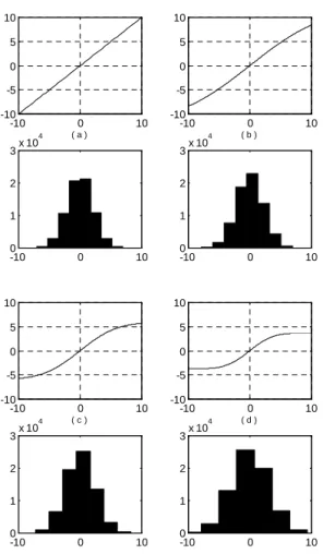
Fig. 11 presents the function g(·) and the histograms

for the amplitude of the nonlinearity input (output of the adaptive filter). The histograms were determined from the signal amplitudes for all the 7000 iterations, averaged over 10 runs (10 realizations). Fig. 11 clearly shows that in cases (b), (c) and (d) the system is driven into a nonlinear region of operation. This emphasizes the importance of analytical models that take into con-sideration the effect of the secondary path nonlinearity whenever it is physically unavoidable in practical appli-cations such as active noise and vibration control.

Table 1 compares the MSE of the converged LMS with the minimum MSE for several degrees of nonlinearity. These values were obtained from (17) and (19) and con-firmed through simulation. The last column shows the corresponding MSE misadjustment.

Table 1: Comparisons between converged LMS and op-timum solutions.

η2 _{Error Surface LMS Misadjustment}

0.1 -21.34 dB -21.27 dB 0.3 %

0.25 -13.6 dB -13.21 dB 2.87 %

0.5 -8.22 dB -6.77 dB 17.64 %

0.75 -5.48 dB -2.35 dB 57.19 %

0.95 -4.07 dB 1.53 dB 137.53 %

1 -3.78 dB -

--10 0 10 -10

-5 0 5 10

( a )

-10 0 10

0 1 2 3x 10

4

-10 0 10

-10 -5 0 5 10

( b )

-10 0 10

0 1 2 3x 10

4

-10 0 10

-10 -5 0 5 10

( c )

-10 0 10

0 1 2 3x 10

4

-10 0 10

-10 -5 0 5 10

( d )

-10 0 10

0 1 2 3x 10

4

Figure 11: Functionsg(·) and respective histograms of

the output of the adaptive filter obtained from simula-tion. (a) η2_{= 0.0005, (b) η}2 _{= 0.05, (c)η}2 _{= 0.2 and} (d)η2_{= 0.5.}

4

SUMMARY

This paper has investigated the properties of the perfor-mance surface for a nonlinear mean-square estimation of a Gaussian random sequence. It expands a previ-ous study, generalizing the statistical characteristics of the input signal. The results of this study have direct application to active noise and vibration control sys-tems when the transducers are driven into a nonlinear behavior and the input signal is correlated. They can be used to evaluate the performance of several methods for determining the optimum controller. A determin-istic expression was derived for the MSE surface as a function of the system’s degree of nonlinearity. It was shown how the nonlinearity deforms the MSE surface. This surface was shown to be unimodal, and the opti-mum weight vector determined. Finally, as an example, the new results were used to quantify the behavior of

ANC systems employing the LMS adaptive algorithm. The MSE misadjustment was evaluated as a function of the degree of nonlinearity. The converged mean weight vector for the LMS was shown to be a scaled version of the optimum weight vector.

ACKNOWLEDGMENTS

This work was supported in part by CAPES (Brazil-ian Ministry of Education) under Grant No. PICDT 0129/97-9, and by CNPq (Brazilian Ministry of Science and Technology) under Grant No. 352084/92-8.

REFERENCES

Angevine, O.L. (1995). Active Systems for attenuation

of Noise. International Journal of Active Control,

1:1, pp. 65-78.

Bernhard, R., P. Davies, and S. Kurth, (1997). Effects of Nonlinearities on System Identification in Active

Noise Control Systems.Proceedings of Noise-Con 97,

Pennsylvania, USA, pp. 231-236.

Bershad N.J., J.J. Shynk and P.L. Feintuch (1993). Sta-tistical Analysis of the Single Layer Backpropagation Algorithm: Part II – MSE and Classification

Per-formance.IEEE Transactions on Signal Processing,

41:2, pp. 583-591.

Costa, M.H., J.C.M. Bermudez, and N.J. Bershad (1999). Statistical Analysis of the LMS Algorithm with a Zero-Memory Nonlinearity after the Adaptive

Filter.Proceedings of ICASSP 99, Phoenix, USA.

Costa, M.H., J.C.M. Bermudez, and N.J. Bershad (2000). The Performance Surface in Nonlinear Mean Square Estimation: Application to the Active Noise

Control Problem. Proceedings of ICASSP 2000,

Is-tambul, Turkey.

F¨uller, C.R. and Flotow, A.H. (1995). Active Control of

Sound and Vibration.IEEE Control Systems, Dec.,

pp. 9-19.

Hansen, C. (1997). Active Noise Control – From

Labo-ratory to Industrial Implementation.Proceedings of

Noise-Con 97, Pennsylvania, USA, pp. 3-38.

Haykin, S. (1996). Adaptive Filter Theory.

Prentice-Hall, third edition.

Kuo, S. and D. Morgan (1996). Active Noise

Massarani, P.M., Zindeluk, M. and Tenenbaum, R. (1990). Realiza¸c˜ao Experimental de Controle Ativo

em Dutos.Proceedings of XI Encontro da Sociedade

Brasileira de Ac´ustica, S˜ao Paulo.

Os´orio, P.O. and N´obrega, M.V. (1995). Controle Ativo

de Ru´ıdo de Banda Larga em Dutos.SBA Controle

& Automa¸c˜ao, 6:2, pp. 70-78.

Papoulis, A. (1991).Probability, Random Variables and

Stochastic Processes. McGraw-Hill, third edition.

Ren, W. and Kumar, P.R. (1992). Stochastic Parallel Model Adaptation: Theory and Applications to Ac-tive Noise Cancelling, Feedforward Control, IIR

Fil-tering and Identification.IEEE Transactions on

Au-tomatic Control, 37:5, pp. 566-578.

Shink, J.J. and N.J. Bershad (1991). Steady-State Anal-ysis of a Single-Layer Perceptron Based on a System

Identification Model with Bias Terms.IEEE