Analytic QCD – a Short Review
Gorazd Cvetiˇca,b∗ and Cristi´an Valenzuelac† aCenter of Subatomic Studies and
bDept. of Physics, Univ. T´ecnica F. Santa Mar´ıa, Valpara´ıso, Chile cDept. of Physics, Pontif. Univ. Cat´olica de Chile, Santiago 22, Chile
(Received on 11 April, 2008)
Analytic versions of QCD are those whose couplingαs(Q2)does not have the unphysical Landau singularities on the space-like axis (−q2=Q2>0). The coupling is analytic in the entire complex plane except the time-like axis (Q2<0). Such couplings are thus suitable for application of perturbative methods down to energies of order GeV. We present a short review of the activity in the area which started with a seminal paper of Shirkov and Solovtsov ten years ago. Several models for analytic QCD coupling are presented. Strengths and weaknesses of some of these models are pointed out. Further, for such analytic couplings, constructions of the corresponding higher order analytic couplings (the analogs of the higher powers of the perturbative coupling) are outlined, and an approach based on the renormalization group considerations is singled out. Methods of evaluation of the leading-twist part of space-like observables in such analytic frameworks are described. Such methods are applicable also to the inclusive time-like observables. Two analytic models are outlined which respect the ITEP Operator Product Expansion philosophy, and thus allow for an evaluation of higher-twist contributions to observables.
Keywords: Analytic coupling; Truncated analytic series (TAS); ITEP-OPE philosophy
I. INTRODUCTION
Perturbative QCD calculations involve coupling a(Q2)≡
αs(Q2)/πwhich has Landau singularities (poles, cuts) on the space-like semiaxis 0≤Q2≤Λ2(q2≡ −Q2). These lead to Landau singularities for the evaluated space-like observables
D
(Q2)at lowQ2∼<Λ2. The existence of such singularities is in contradiction with the general principles of the local quan-tum field theories [1]. Further, lattice simulations [2] confirm that such singularities are not present ina(Q2).An analytized coupling
A
1(Q2), which agrees with the per-turbativea(Q2) atQ2→∞and is analytic in the Euclidean part of theQ2-plane (Q2εC
,Q26≤0), addresses this problem, and has been constructed by Shirkov and Solovtsov about ten years ago [3].Several other analytic QCD (anQCD) models for
A
1(Q2) can be constructed, possibly satisfying certain additional con-straints at low and/or at highQ2.Another problem is the analytization of higher power terms an7→
A
nin the truncated perturbation series (TPS) forD
(Q2). Also here, several possibilities appear.Application of the Operator Product Expansion (OPE) ap-proach, in the ITEP sense, to inclusive space-like observables appears to make sense only in a restricted class of such an-QCD models.
This is a short and incomplete review of the activity in the area; relatively large space is given to the work of the re-view’s authors. For an earlier and more extensive review, see e. g. Ref. [4].
Section II contains general aspects of analytization of the Euclidean couplinga(Q2)7→
A
1(Q2), and the definition of the time-like (Minkowskian) couplingA1(s). Further, in Sec. II∗Electronic address:[email protected] †Electronic address:[email protected]
we review the minimal analytization (MA) procedure devel-oped by Shirkov and Solovtsov [3], and a variant thereof de-veloped by Nesterenko [5]. In Sec. III we present various approaches of going beyond the MA procedure, i.e., various models forA1(s), and thus for
A
1(Q2)[6–11]. In Sec. IV, analytization procedures for the higher powers an(Q2)7→A
n(Q2)in MA model are presented [12–14], and an alterna-tive approach which is applicable to any model of analyticA
1(Q2)[10, 11] is presented. In Sec. V, an analytization of noninteger powersaν(Q2)is outlined [15]. In Sec. VI, meth-ods of evaluations of space-like and of inclusive time-like ob-servables in models with analyticA
1(Q2)are described, and some numerical results are presented for semihadronicτ de-cay rate ratiorτ, Adler functiondv(Q2)and Bjorken polarized sum rule (BjPSR)db(Q2)[10–14, 16]. In Sec. VII, two sets of models are presented [17, 18] whose analytic couplingsA
1(Q2)preserve the OPE-ITEP philosophy, i.e., at highQ2 they fulfill:|A
1(Q2)−a(Q2)|<(Λ2/Q2)kfor anykεN
. Sec-tion VIII contains a summary of the presented themes.II. ANALYTIZATIONa(Q2)7→A
1(Q2)
In perturbative QCD (pQCD), the beta function is written as a truncated perturbation series (TPS) of couplinga. There-fore, the renormalization group equation (RGE) fora(Q2)has the form
∂a(lnQ2;β2, . . .)
∂lnQ2 = −
jmax
∑
j=2
βj−2aj(lnQ2;β2, . . .). (1)
perturbative RGE (1) can be written in the form
a(Q2) =
∞
∑
k=1 k−1
∑
ℓ=0 Kkℓ(ln
L)ℓ
Lk , (2)
where L=ln(Q2/Λ2) and K
kℓ are constants depending on
βj’s. In MS:Λ=Λ∼10−1GeV.
The pQCD couplinga(Q2)is nonanalytic on−∞<Q2≤
Λ2. Application of the Cauchy theorem gives the dispersion relation
a(Q2) =1
π
Z ∞
σ=−Λ2−η
dσρ(1pt)(σ)
(σ+Q2) , (η→0), (3) whereρ(1pt)(σ)is the (pQCD) discontinuity function ofaalong the cut axis in theQ2-plane: ρ(1pt)(σ) =Ima(−σ−iε). The MA procedure of Shirkov and Solovtsov [3] removes the pQCD contribution of the unphysical cut 0<−σ≤Λ2, keep-ing the discontinuity elsewhere unchanged (“minimal analyti-zation” ofa)
A
1(MA)(Q2) =1π
Z ∞
σ=0
dσρ(1pt)(σ)
(σ+Q2) . (4) In general:
A
1(Q2) =1
π
Z ∞
σ=0
dσρ1(σ)
(σ+Q2), (5) whereρ1(σ) =Im
A
1(−σ−iε). Relation (5) defines an ana-lytic coupling in the entire Euclidean complexQ2-plane, i.e., excluding the time-like semiaxis−s=Q2≤0. On this semi-axis, it is convenient to define the time-like (Minkowskian) couplingA1(s)[12–14]A1(s) = i
2π Z −s−iε
−s+iε
dσ′
σ′
A
1(σ′). (6)The following relations hold between
A
1,A1andρ1:A1(s) = 1
π
Z ∞
s dσ
σ ρ1(σ), (7)
A
1(Q2) = Q2Z ∞
0
dsA1(s)
(s+Q2)2 , (8) d
dlnσA1(σ) = −
1
πρ1(σ). (9)
The MA is equivalent to the minimal analytization of the TPS form of theβ(a) =∂a(Q2)/∂lnQ2function [19]
∂A1(MA)(lnQ2;β2, . . .)
∂lnQ2 =
1
π
Z ∞
σ=0
dσρ(βpt)(σ) (σ+Q2) , (10) whereρ(βpt)(σ) =Imβ(a)(−σ−iε), and
β(a) = − jmax
∑
j=2
βj−2aj(lnQ2;β2, . . .). (11)
0.0 0.5 1.0 1.5 2.0 2.5 3.0 0.00
0.25 0.50 0.75 1.00 1.25 1.50
Q(GeV)
®E
¤ = 400 MeV
¤ = 200 MeV
®{s
0.0 0.2 0.4 0.6 0.8 1.0 Q(GeV) 0.0
0.5 1.0 1.5
1-loop
2 3-loop,
Analytic running coupling
FIG. 1:Left: one-loop MAαE(Q) =πA1(Q2)and its one-loop perturbative counterpartαs(Q2)in MS, fornf=3 andΛ=Λ=0.2 and 0.4 GeV. Right:
stability of the MAαE(Q) =πA1(Q2)under the loop-level increase. Both figures from: Shirkov and Solovtsov, 1997 [3].
10 Q(GeV) 5 0 5 10
0.0 0.5 1.0 1.5
(GeV)
s1/2
®{(2)s (Q2; 3)
A(1)(Q2; 3)
A(2,3) A(2,3)
A(1)(s; 3)
A1(0) =A1(0)
FIG. 2:The MA time-like and space-like couplingsA1(s1/2)andA 1(Q)at 1-loop, 2-loop (3-loop) level; in MS fornf=3 andΛ=0.35 GeV [A1and A1in figure areπA1andπA1in our normalization convention]. Figure from: Shirkov and Solovtsov, 2006 [16].
The MA couplings
A
1(Q2)andA1(s)are finite in the IR (with the value 1/β0 atQ2=0, ors=0) and show strong stabil-ity under the increase of the loop-level nm= jmax−1 (see Figs. 1, 2), and under the change of the renormalization scale (RScl) and scheme (RSch). Another similar pQCD-approach is to analytize minimallyβ(a)/a=∂lna(Q2)/∂lnQ2[5, 20, 21]. This leads to an IR-divergent analytic (MA) coupling,A
1(Q2)∼(Λ2/Q2)(ln(Λ2/Q2))−1 when Q2→0. At one-loop:A
1(Q2) =1
β0
(Q2/Λ2)−1
(Q2/Λ2)ln(Q2/Λ2) . (12)
FIG. 3: Left: one-loop MAeαan(Q) =β0A1(Q2)and its one-loop perturba-tive counterpart, as a function ofZ=Q2/Λ2(Figure from: Nesterenko, 2000 [5]). Right: stability of the MAαean(Q) =β0A1(Q2)under the loop-level increase, as a function ofZ=Q2/Λ2(Figure from: Nesterenko, 2001 [20]).
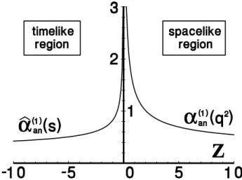
FIG. 4:One-loop time-like and space-like MA couplings ˆαan(s) =πA1(s) andαan(Q2) =πA1(Q2)as a function ofZ=−s/Λ2orZ=Q2/Λ2, respec-tively. Figure from: Nesterenko, 2003 [21].
III. BEYOND THE MA
The idea to make the QCD coupling IR finite phenomeno-logically is an old one, by the substitution ln(Q2/Λ2)7→ ln[(Q2+4mg2)/Λ2] where mg is an effective gluon mass, cf. Refs. [22–24].
On the other hand, the analytic MA, or MA, couplings can be modified at low energies, bringing in additional parame-ter(s) such that there is a possibility to reproduce better a wide set of low energy QCD experimental data.
Among the recent proposed analytic couplings are: 1. Synthetic coupling proposed by Alekseev [6]:
αsyn(Q2) =α(MA)(Q2) +
π β0
·
cΛ2 Q2 −
dΛ2 Q2+m
g2
¸
, (13)
where the three new parametersc,d and gluon massmgwere determined by requiringαsyn(Q2)−αpt(Q2)∼(Λ2/Q2)3(for the convergence of the gluon condensate) and by the string conditionV(r)∼σr(r→∞) withσ≈0.422GeV2. This cou-pling is IR-divergent.
2. The coupling by Sriwastawaet al.[7]: 1
α(SPPW1) (Q2)= 1
α(SPPW1) (Λ2)
+β0
π ∞ Z
0
(z−1)zp
(σ+z−iε)(σ+1)(1+zp)dσ, (14) wherez=Q2/Λ2and 0<p≤1. This formula coincides with Nesterenko’s (one-loop) MA coupling whenp=1.
3. An IR-finite coupling proposed by Webber [8]:
α(W1)(Q2) = π
β0 ·
1 lnz+
1 1−z
z+b 1+b
µ 1+c z+c
¶p¸
, (15)
wherez=Q2/Λ2and specific values are chosen for parame-tersb=1/4,c=4, andp=4;αW(1)(0)≃π/(2β0).
4. “Massive” MA or MA couplings
A
1(Q2)andA1(s) pro-posed by Nesterenko and Papavassiliou [9]:A1(m)(s) = Θ(s−4m2)A1(s),
A
1(m)(Q2) =Q2 Q2+4m2
Z ∞
4m2ρ1(σ)
σ−4m2
σ+Q2 dσ
σ ,
(16)
wherem∼Λ; andρ1(σ) =ρ1(pt)(σ)in the MA case. In this case:
A
1(m)(0) =A1(m)(0) =0. The massmis some kind of threshold, and can be expected to be∼mπ.5. Two specific models of IR-finite analytic coupling [10, 11]: on the time-like axiss≡ −Q2>0, the parturbative discontinuity functionρ1(s), or equivalently A1(MA)(s), was modified in the in the IR regime (s∼Λ2). A first possibility (model ’M1’):
A(M1)
1 (s) = cfM 2 rδ(s−M
2 r)
+k0Θ(M20−s) +Θ(s−M 2 0)A
(MA)
1 (s), wherecf,k0,cr=M
2 r/Λ
2
,c0=M 2 0/Λ
2
are four dimension-less parameters of the model, all∼1. One of them (k0) can be eliminated by requiring the (approximate) merging of M1 with MA at largeQ2:
|
A
1(M1)(Q2)−A
1(MA)(Q2)| ∼(Λ 2/Q2)2.
The Euclidean
A
1(M1)(Q2)isA
1(M1)(Q2) =A
1(MA)(Q2) +∆A1(M1)(Q2),∆A1(M1)(Q2) = −π1
Z M20
σ=0
dσρ(1pt)(σ) (σ+Q2) +cf
M2rQ2
³
Q2+M2 r
´2
−df M20
³
Q2+M2 0
´, (17)
where the constantdf is df ≡ −k0+
1
π
Z ∞
M20
dσ σ ρ
(pt)
Another, simpler, possibility is (model ’M2’):
A(M1)
1 (s) = A
(MA)
1 (s) +cvΘ(M 2
p−s), (18)
A
1(M1)(Q2) =A
1(MA)(Q2) +cvM2p
(Q2+M2 p)
, (19)
wherecvandcp=M 2 p/Λ
2
are the model parameters.
6. Those anQCD models which respect the OPE-ITEP con-dition are presented in Sec. VII.
IV. ANALYTIZATION OF HIGHER POWERSak7→Ak
In MA model, the construction is [3, 12–14] (MSSSh: Mil-ton, Solovtsov, Solovtsova, Shirkov):
ak(Q2)7→
A
k(MA)(Q2) = 1π
Z ∞
0 dσ σ+Q2ρ
(pt)
k (σ), (20) wherek=1,2, . . .;ρ(kpt)(σ) =Im[ak(−σ−iε)]; andais given, e.g., by Eq. (2). In other words, “minimal analytization” (MA) is applied to each powerak.
As a consequence, in MA we have [19]
∂A1(MA)(µ2)
∂lnµ2 = −β0
A
(MA)
2 (µ2)−β1
A
3(MA)(µ2)−···,∂2
A
(MA) 1 (µ2)∂(lnµ2)2 = 2β 2 0
A
(MA)
3 +5β0β1
A
4(MA)+···,etc. This is so becauseak, and consequentlyρ(pt)
k (σ), fulfill analogous RGE’s.
The approach (20) of constructing
A
k’s (k≥2) can be ap-plied to a specific model only (MA). In other anQCD models (i.e., for otherA
1(Q2)), the discontinuity functionsρk(k≥2) are not known. We present an approach [10, 11] that is plicable to any anQCD model, and reduces to the above ap-proach in the MA model. We proposed to maintain the scale (RScl) evolution of these (truncated) relations for any version of anQCD∂A1(µ2;β2, . . .)
∂lnµ2 = −β0
A
2− ··· −βnm−2A
nm,∂2
A
1(µ2;β2, . . .)
∂(lnµ2)2 = 2β 2
0
A
3+5β0β1A
4+···+κ(n2m)A
nm, (21)etc. Eqs. (21) define the couplings
A
k(Q2)(k≥2). Further, the evolution under the scheme (RSch) changes will also be maintained as in the MA case (and in pQCD):∂A1(µ2;β2, . . .)
∂β2 ≈
1
β0
A
3+β2 3β2
0
A
5+···+k(n2m)A
nm, (22)analogously for ∂A1/∂β3, etc. In our approach, the basic space-like quantities are
A
1(µ2) of a given anQCD model(e.g., MA, M1, M2) and its logarithmic derivatives
e
A
n(µ2)≡(−1)n−1
βn−1 0 (n−1)!
∂n−1
A
1(µ2)∂(lnµ2)n−1 , (n=1,2, . . .), (23) whose pQCD analogs are
e
an(µ2)≡
(−1)n−1
βn0−1(n−1)!
∂n−1a(µ2)
∂(lnµ2)n−1 , (n=1,2, . . .). (24) At loop-level three (nm=3), where we include in RGE (1) term withjmax=4 (thusβ2), relations (21) are
e
A
2(µ2) =A
2(µ2) +β1
β0
A
3(µ2),A
e3(µ2) =A
3(µ2), (25)implying
A
2(µ2) =A
e2(µ2)−β1
β0 e
A
3(µ2),A
3(µ2) =A
e3(µ2). (26)The RSch (β2) dependence is obtained from the truncated Eqs. (22) and (21)
∂
A
ej(µ2;β2)∂β2 ≈
1 2β3
0
∂2
A
ej(µ2;β2)
∂(lnµ2)2 , (27)
where(j=1,2, . . .)and
A
e1≡A
1.At loop-level four (nm=4), where we include in RGE (1) term withjmax=5 (thusβ3), relations analogous to (26)-(27) can be found [11].
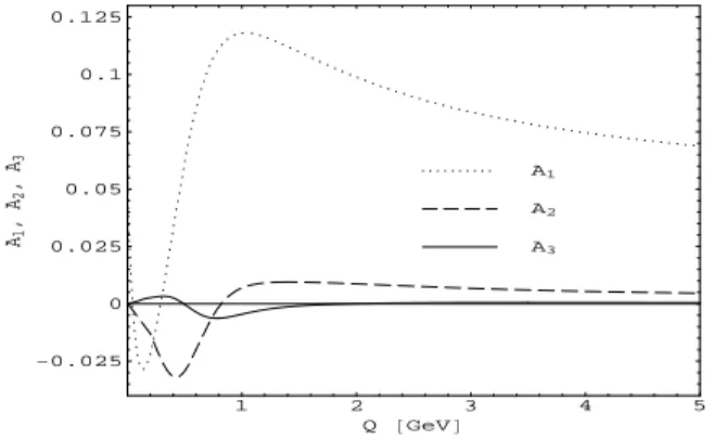
It turns out that there is a clear hierarchy in magnitudes |
A
1(Q2)|>|A
2(Q2)|>|A
3(Q2)|>···at allQ2, in all or most of the anQCD models (cf. Fig. 5 for MA, M1, M2; and Fig. 9 in Sec. VII for another model).0.5 1 1.5 2 2.5 3 3.5 4
Q@GeVD -0.1
0 0.1 0.2 0.3 0.4
A1
,
3
A2
loop-level=4,kmax=6, A RSch
3A2,M2
3A2,M1 3A2,MA A1, M2 A1, M1 A1, MA
FIG. 5: A1 andA2 for various models (M1, M2 and MA) with specific model parameters:c0=2.94,cr=0.45,cf=1.08 for M1;cv=0.1,cp=3.4
for M2;nf =3,Λ(nf=3)=0.4 GeV in all three models. The upper three
curves areA1, the lower three are 3×A2. All couplings are in v-scheme (see Subsec. VI A).A2is constructed with our approach. Figure from: Ref. [11].
We recall that the perturbation series of a space-like observ-able
D
(Q2)(Q2≡ −q2>0) can be written asD
(Q2)pt = a+d1a2+d2a3+···, (28)= ae1+d1ea2+ µ
d2−
β1
β0 d1
¶ e
where the second form (29) is the reorganization of the per-turbative power expansion (28) into a perturbation expansion in terms ofaen’s (24) (note: ea1≡a). The basic analytization rule we adopt is the replacement
e
an7→
A
en (n=1,2, . . .), (30) term-by-term in expansion (29), and this is equivalent to the analytization rule an7→A
n term-by-term in expansion (28). However, in principle, other analytization procedures could be adopted, e.g. an7→
A
n1, oran7→
A
1A
n−1, etc. The described analytizationan7→A
nreduces to the MSSSh analytization in the case of the MA model (i.e., in the case ofA
1=A
(MA)
1 ), because the aforementioned RGE-type relations hold also in the MA case.
Let’s denote by
D
(nm)(Q2)the TPS of (28) with terms up to (and including) the term∼anm, and byD
(nm)an. (Q2)the cor-responding truncated analytic series (TAS) obtained from the previous one by the term-by-term analytizationan7→
A
n. The evolution of
A
k(Q2)under the changes of the RSch was trun-cated in such a way that ∂D(nm)an. (Q2)/∂βj ∼
A
nm+1 (wherej≥2). Further, our definition of
A
k’s (k≥2) via Eqs. (21) [cf. Eqs. (26)] involves truncated series which, however, still ensure the “correct” RScl-dependence∂D(nm)an. (Q2)/∂µ2∼
A
nm+1. This is all in close analogy with the pQCD results for TPS’s:∂D(nm)(Q2)/∂βj∼anm+1, and∂D(nm)(Q2)/∂µ2∼ anm+1. In conjunction with the mentioned hierarchy depicted in Fig. 5, this means that the evaluated TAS will have increas-ingly weaker RSch and RScl dependence when the number of TAS terms increases, at all values ofQ2.
On the other hand, if the analytization of powers were per-formed by another rule, for example, by the simple rulean7→
A
n1, the above RScl&RSch-dependence of the TAS would not be valid any more. An increasingly weaker RScl&RSch-dependence of TAS (when the number of TAS terms is in-creased) would not be guaranteed any more.
V. CALCULATION OFAνFORνNONINTEGER
Analytization of noninteger powers in MA model was per-formed and used in Refs. [15], representing a generalization of results of Ref. [25]. The approach was motivated by a previ-ous work [26] where MA-type of analytization of expressions for hadronic observables was postulated, these being integrals linear ina(tQ2)[similar to the dressed gluon approximation expressions, cf. Eq. (44) and the first line of Eq. (48)]. Ana-lytization of noninteger powersaνoraνlna, is needed in cal-culations of pion electromagnetic form factor, and in some re-summed expressions for Green functions or observables, cal-culated within an anQCD model.
In the mentioned approach, use is made of the Laplace transformation(f)Lof function f
f(z)7→(f)L(t): f(z) =
Z ∞
0
dte−zt(f)L(t), wherez≡ln(Q2/Λ2). Using notations (24) and (23), it can be
shown
(aen)L(t) =
tn−1
βn−1 0 (n−1)!
(a)L(t), (31)
(
A
en)L(t) =tn−1
βn0−1(n−1)!(
A
1)L(t). (32) Therefore, it is natural to define for any realνthe following Laplace transforms:(aeν)L(t) =
tν−1
βν−1 0 Γ(ν)
(a)L(t); (33)
(
A
eν)L(t) =tν−1
βν0−1Γ(ν)(
A
1)L(t). (34) In MA model, at one-loop level, (a)L(t) and (A
1)L(t) are knowna(z) = 1
β0z ⇒
(a)L(t) = 1
β0
. (35)
A
1(z) =1
β0 µ
1 z−
1 ez−1
¶
⇒
(
A
1)L(t) = 1β0 Ã
1−
∞
∑
k=1
δ(t−k) !
. (36)
Since at one-loop
A
eν=A
ν, it follows in one-loop MA modelA
ν(z) =Z ∞
0
dte−zt t
ν−1
βν0Γ(ν) Ã
1−
∞
∑
k=1
δ(t−k) !
. (37)
Similarly, since
aν(z)lna(z) = d
dνa ν(z),
it can be defined ·
d dνa
ν(z)
¸
MA
≡ddν
A
ν(z). (38)To calculate higher (two-)loop level
A
ν(z)in MA model, theauthors of Refs. [15] expressed the two-loopa(2)(z)in terms of one-loop powersa(1)m(z)lnna(1)(z)and then followed the
above procedure.
VI. EVALUATION METHODS FOR OBSERVABLES
space-like physical scaleQ2(≡ −q2)>0. Its usual perturba-tion series has the form (28), wherea=a(µ2;β2,β3, . . .), with µ2∼Q2. For each TPS
D
(Q2)(ptN) of orderN, in the minimal anQCD (MA) model, the authors MSSSh [12–14] introduced the aforementioned replacementan7→A
(MA)n :
D
(Q2)an(N)(MSSSh)=A
1(MA)+d1A
2(MA)+···dN−1A
N(MA). (39) This method of evaluation (viaan→A
n) was extended to any anQCD model in [10, 11] (cf. Sec. IV). Further, in the case of inclusive space-like observables, the evaluation was extended to the resummation of the large-β0terms:A. Large-β0-motivated expansion of observables
We summarize the presentation of Ref. [11]. We work in the RSch’s where each βk (k≥2) is a polynomial innf of orderk; in other words, it is a polynomial inβ0:
βk= k
∑
j=0
bk jβ0j, k=2,3, . . . (40)
The MS belongs to this class of schemes. In such schemes, the coefficientsdnof expansion (28) have the following specific form in terms ofβ0:
D
(Q2)pt=a+ (c11β0+c10)a2+(c22β20+c21β0+c20+c2,−1β−01)a3+···. (41) We can construct a separation of this series into a sum of two RScl-independent terms – the leading-β0(Lβ0), and beyond-the-leading-β0(BLβ0)
D
pt =D
pt(Lβ0)+D
(BLβ0)
pt , (42)
where
D
(Lβ0)pt =a+a2[β0c11] +a3£β20c22+β1c11¤ +a4
·
β30c33+ 5
2β0β1c22+β2c11 ¸
+
O
(β40a5). (43)Expression (43) is not the standard leading-β0 contribution, since it contains also terms withβj(j≥1), but only in a mini-mal way to ensure that the expression contains all the
leading-β0terms and at the same time remains RScl-independent. It can be shown that, for inclusive observables, all the coeffi-cients in this Lβ0 contribution can be obtained, and can be expressed in the integral form [27]
D
(Lβ0)(Q2) pt=Z ∞
0 dt
t F
E
D(t)a(teCQ2), (44)
whereFDE(t)is the (Euclidean) Lβ0 -characteristic function. In MS scheme, Λ=Λwhich corresponds here to
C
=C
≡−5/3. No RSclµ2appears in (44). Expression (44) is referred to in the literature sometimes as dressed gluon approximation.
The BLβ0contribution is usually known only to ∼a3 or ∼a4. For it, we can use an arbitrary RSclµ2≡Q2eC∼Q2. Further, the powersakcan be reexpressed in terms ofae
n(µ2) (24):
a2=ea2−(β1/β0)ae3+···, a3=ae3+···. (45) Therefore,
D
(Q2)(TPS)=D
(Lβ0)(Q2)pt+et2ae2(Q2eC) +et3ae3(Q2eC) +et4ae4(Q2eC), (46) whereet2=c10is scheme-independent, and coefficientset3and e
t4have a scheme dependence (depend onβ2,β3– i.e., onb2j andb3j). We note that expression (46) is not really a pure TPS, because its Lβ0contribution (43) is not truncated. An observable-dependent scheme (D-scheme) can be chosen such thatet3=et4=0. For the Adler function
D
=dv, such a scheme will be called v-scheme. The analytization of the obtainedD
(Q2)(TPS) (46) is performed by the substitution aen7→A
en, Eq. (30), leading to the truncated analytic series (TAS)D
(Q2) =D
(Q2)(TAS)+O
(β30A
e5), (47)D
(Q2)(TAS)=Z ∞
0 dt
t F
E
D(t)
A
1(teCQ2)+c10
A
e2(Q2eC)+et3A
e3(Q2eC)+et4A
e4(Q2eC). (48) In the D-scheme, the last two terms disappear. Eq. (48) is a method that one can use to evaluate any inclusive space-like QCD observable in any anQCD model. As argued in Sec. IV, the scale and scheme dependence of the TAS is very suppressed∂D(Q2)(TAS)
∂X ∼β
3
0
A
e5∼β30A
5 (X=lnµ2,βj). (49) If the BLβ0perturbative contribution is known exactly only up to (and including)∼a3, then noet4term appears in Eq. (48) and the precision in Eqs. (47) and (49) is diminished:
O
(β30
A
5)7→O
(β20
A
4).It is interesting to note that the Taylor expansion of
A
1(teCQ2) inD
(Lβ0)(Q2)an in (48) around a chosen RScl ln(µ2)reveals just the aforementionedan7→A
nanalytization of the large-β0part (43), in any anQCD:D
(Lβ0) an =Z ∞
0 dt
t F
E
D(t)
A
1(teCQ2) =A
1+A
2[β0c11] +A
3£
β2
0c22+β1c11 ¤
+
A
4 ·β30c33+ 5
2β0β1c22+β2c11 ¸
+
O
(β40A
5),where
A
k=A
k(µ2;β2,β3, . . .). In other words, at theleading-β0 level, the natural analytization a7→
A
1 in integral (44) is equivalent to the term-by-term analytizationan7→A
n(⇔e
an7→
A
en) in the corresponding perturbation series. This thus represents yet another motivation for the analytizationan7→TABLE I: Various order contributions to observables within PT, and MSSSh (=APT) methods [14, 16]:
Process Method 1st order 2nd 3rd
GLS PT 65.1% 24.4% 10.5%
(Q∼1.76GeV) APT 75.7% 20.7% 3.6%
rτ PT 54.7% 29.5% 15.8%
(Mτ=1.78GeV) APT 87.9% 11.0% 1.1%
B. Applications in phenomenology
Evaluations in MA model, with the MSSSh-approachan7→
A
n(MA) [12–14], are usually performed in MS scheme. The only free parameter isΛ(=Λ). Fitting the experimental data for ϒ-decay,Z→hadrons,e+e−→hadrons, to the MSSSh approach for MA at the two- or three-loop level, they obtainedΛnf=5≈0.26-0.30 GeV, corresponding to:Λnf=3≈0.40-0.44
GeV, andπ
A
1(MA)(MZ2)≈0.124, which is above the pQCD world-average valueαs(M2Z)≈0.119±0.001. The apparent convergence of the MSSSh nonpower truncated series is also remarkable – see Table I.In Refs. [10, 11], the aformentioned TAS evaluation method (48) in anQCD models MA (4), M1 (17) and M2 (19) was ap-plied to the inclusive observables Bjorken polarized sum rule (BjPSR) db(Q2), Adler function dv(Q2) and semihadronic
τ decay ratio rτ The exact values of coefficients d1 and d2 are known for space-like observables BjPSRdb(Q2)[28] and (massless) Adler functiondv(Q2)[29, 30]. (The exact coeffi-cientd3ofdvhas been recently obtained [31], but was not in-cluded in the analysis of Ref. [11] that we present here; rather, an estimated value ofd3was used.) In the v-scheme, the eval-uated masslessdv(Q2)is
dv(Q2)(TAS) =
Z ∞
0 dt
t F
E
v (t)
A
1(teCQ2;β2(x),β3(x)) +112
A
e2(eC
Q2), (50)
while BjPSRdb(Q2)
(TAS)has one more termet3
A
e3(eCQ2). The difference between the (massless) truedx(Q2)(x=v,b) and dx(Q2)(TAS)isO
(β20A
e4). The semihadronicτdecay ratiorτis,on the other hand, a time-like quantity, but can be expressed as a contour integral involving the Adler functiondv:
rτ(∆S=0,mq=0) = 2
π Z mτ2
0 ds mτ2
µ 1− s
mτ2
¶2µ 1+2 s
mτ2
¶
ImΠ(s) =
1 2π
Z +π
−π
dφ(1+eiφ)3(1−eiφ)d
v(Q2=mτ2eiφ). (51)
This implies for the leading-β0term ofrτ
rτ(∆S=0,mq=0)(Lβ0)=
Z ∞
0 dt
t F
M
r (t)A1(teCmτ2), (52)
where A1 is the time-like coupling appearing in Eqs.
(6)-(9), and superscript
M
in the characteristic function indicatesTABLE II: Results of evaluation of rτ(△S=0,mq =0) and of
BjPSRdb(Q2) (Q2=2 and 1GeV2), in various anQCD models, using TAS method (48). The experimental values are rτ(△S=
0,mq=0) =0.204±0.005,db(Q2=2 GeV2) =0.16±0.11 and db(Q2=1 GeV2) =0.17±0.07.
rτ db(Q2=2) db(Q2=1)
MA 0.141 0.137 0.155
M1 0.204 0.160 0.170
M2 0.204 0.189 0.219
that it is Minkowskian (time-like). The latter was obtained by Neubert (second entry of Refs. [27]). The beyond-the-leading-β0(BLβ0) contribution is the contour integral
rτ(△S=0,mq=0)(BLβ0)= 1
24π
Z +π
−π
dφ(1+eiφ)3(1−eiφ)e
A
2(eCmτ2eiφ). (53)
The parameters of anQCD models M1 (17) and M2 (19) were
-0.2 -0.1 0 0.1 0.2 0.3 0.4 0.5
0.4 0.6 0.8 1 1.2 1.4 1.6 1.8 2
dv
(Q
2 )
Q [GeV] exp.
loop-level=4, kmax=6
Λ= 0.4 GeV M1: c0=2.94, cr=0.45, cf=1.08
M2: cv=0.1, cp=3.4
MA,M1,M2: µ2=Q2 e-5/3 (massless p.)
mass corr. and STPS: µ2=Q2
M1 MA M2
STPS’s
(b)
full quantities
exp.
STPS 4-l.(bMS) STPS 3-l.(bMS) M2 (A) M1 (A) MA (A) exp.
FIG. 6:Adler function as predicted by pQCD, and by our approach in sev-eral anQCD models: MA, M1, M2. The full quantity is depicted, with the contribution of massive quarks included. The experimental values are from [32]. Figure from: Ref. [11].
then determined [11] by fitting the evaluated observables to the experimental central valuesrτ(△S=0,mq=0) =0.204 (for M1 and M2), and todb(Q2=1GeV2) =0.17 andd
b(Q2= 2) =0.16 (for M1). For M1 we obtained: cf =1.08,cr = 0.45,c0=2.94. For M2 we obtained:cv=0.1 andcp=3.4.
The numerical results were then obtained [11]. In models MA, M1 and M2 they are given forrτin Table II, for Adler functiondv(Q2)in Fig. 6, and for BjPSRdb(Q2)(in M1 and M2) in Figs. 7 and 8 (Table II and Figs. 6, 7, 8 are taken from Ref. [11]). All results were calculated in the v-scheme. For details, we refer to Ref. [11].
0.1 0.11 0.12 0.13 0.14 0.15 0.16 0.17
1 1.5 2 2.5 3 3.5 4
db
(Q
2)
Q [GeV]
loop-level= 3
kmax=5
Λ= 0.4 GeV µ2=Q2
e-5/3
M1 sk
(B) (A) (Q2,B)
(Q2,A)
LS(B) LS(A)
M1: c0=2.94, cr=0.45, cf=1.08
(a)
LS (A) LS (B) µ2=Q2 (A)
µ2=Q2
(B) (A) (B) sk (A)
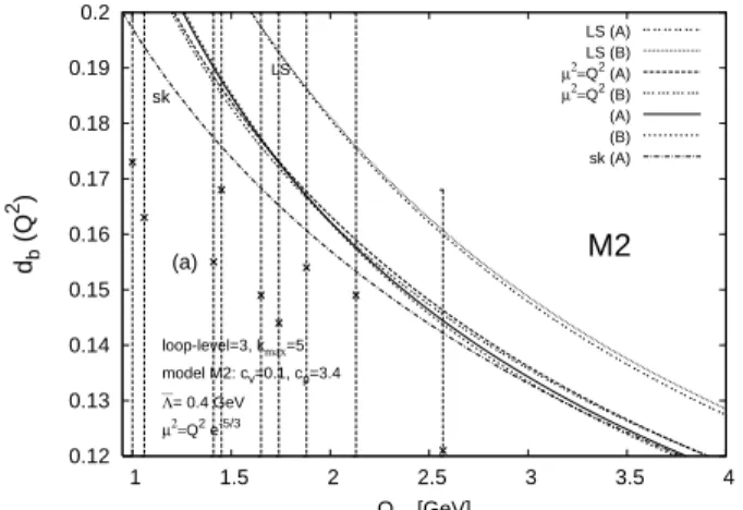
FIG. 7:Bjorken polarized sum rule (BjPSR)db(Q2)in model M1, in various
RSch’s and at various RScl’s. The vertical lines represent experimental data, with errorbars in general covering the entire depicted range of values.
0.12 0.13 0.14 0.15 0.16 0.17 0.18 0.19 0.2
1 1.5 2 2.5 3 3.5 4
db
(Q
2)
Q [GeV]
loop-level=3, kmax=5
model M2: cv=0.1, cp=3.4
Λ= 0.4 GeV µ2=Q2 e-5/3
sk
LS
M2 (a)
LS (A) LS (B) µ2=Q2
(A) µ2=Q2
(B) (A) (B) sk (A)
FIG. 8: As in the Fig. 7, but this time for model M2. Both figures from: Ref. [11].
tal mass spectrum was used to extract the approximate val-ues of the (analytic) coupling
A
1(Q2)at lowQ2. In this for-malism, the current quark masses were replaced by the con-stituent quark masses, accounting in this way approximately for the quark self-energy effects. The results by the authors of Ref. [34] indicate thatA
1(Q2)remains finite (and becomes possibly zero) whenQ2→0.VII. ANALYTIC QCD AND ITEP-OPE PHILOSOPHY
In general, the deviations of analytic
A
1(Q2)from the per-turbative couplingapt(Q2)at highQ2≫Λ2are power terms|δA1(Q2)| ≡ |
A
1(Q2)−apt(Q2)| ∼ µΛ2 Q2
¶k
(Q2≫Λ2),
wherekis a given positive integer. Such a coupling introduces in the evaluation (of the leading-twist) of inclusive space-like observables
D
(Q2), already at the leading-β0 level, an UV contribution δD(UV)(Q2) which behaves like a power term
[18]
δD(UV)(Q2)∼
µ
Λ2 Q2
¶min(k,n)
ifk6=n, (54) wheren ε
N
is the position of the leading IR renormalon of the observableD
(Q2); ifk=n, then the left-hand side of Eq. (54) changes to(Λ2/Q2)nln(Λ2/Q2)[18]. Such nonper-turbative contributions coming from the UV sector contradict the ITEP Operator Product Expansion (OPE) philosophy (the latter saying that such terms can come only from the IR sector) [35].Two specific sets of models of anQCD have been intro-duced in the literature so far such that they do not contradict the ITEP-OPE:
(A) a model set based on a modification of theβ(a)function [17];
(B) a model set obtained by a direct construction [18].
A. Set of models A
This is the set of models constructed in Refs. [17]. The TPS
β(a)used in pQCD is
∂a
∂lnQ2=β
(N)(a) =−β
0a2 Ã
1+
N
∑
j=1 cjaj
!
. (55)
This was then modified,β(N)(a)7→eβ(N)(a), by fulfilling three
main conditions:
1.) eβ(N)(a) has the same expansion in powers of a as
β(N)(a);
2.) eβ(N)(a)∼ −ζap withζ>0 and p≤1, fora≫1, in order to ensure the absence of Landau singularities;
3.)eβ(N)(a)is analytic function ata=0, in order to ensure
|a(Q2)−apt(Q2)|<(Λ2/Q2)kfor anyk>0 at largeQ2(thus respecting the ITEP-OPE approach).
This modification was performed by the substitutiona7→ u(a)≡a/(1+ηa),η>0 being a parameter, and
e
β(N)(a) = −β0 "
κ(a−u(a))+
N
∑
j=0 e
cju(a)j+2
#
, (56)
andecjare adjusted so that the first condition is fulfilled e
c0=1−ηκ, ce1=c1+2η−η2κ, etc.
B. Set of models B
This is the set of models for
A
1constructed in Ref. [18]. A class of IR-finite analytic couplings which respect the ITEP-OPE philosophy can be constructed directly. The proposed class of couplings has three parameters (η,h1,h2). In the in-termediate energy region (Q∼1 GeV), the proposed coupling has low loop-level and renormalization scheme dependence. We outline here the construction. We recall expansion (2) for the perturbative couplinga(Q2), whereL=logQ2/Λ2andKkℓ are functions of the β-function coefficients. This expansion (sum) is in practice usually truncated in the indexk(k≤km). The proposed coupling is obtained by modifying (the
nonan-1 2 3 4 5
Q @GeVD
-0.025 0 0.025 0.05 0.075 0.1 0.125
A1
,
A2
,
A3
A3
A2
A1
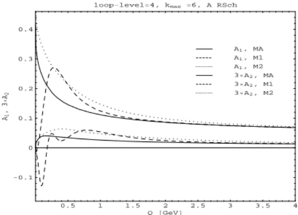
FIG. 9:The couplingsA2andA3, together with the corresponding coupling A1, are plotted as a function ofQ, in the MS-scheme, withΛ=0.4 GeV. The parameters used for the couplings areη=0.3,h1=0.1, andh2=0. Figure from: Ref. [18].
alytic)L’s to analytic quantitiesL0andL1that fall faster than any inverse power of Q2 at large Q2, and by adding to the truncated sum another quantity with such properties:
A
1(km)(Q2) = km∑
k=1 k−1
∑
ℓ=0
Klℓ(logL1) ℓ Lk0 +e
−η√xf(x), (57)
wherex=Q2/Λ2. The second term is only relevant in the IR region, and the first term (double sum) plays, in the UV region, the role of the perturbative coupling. L0 andL1are analytic and chosen aiming at a lowkm-dependence in the IR region.
1 Li
=1
L+
eνi(1−√x)
1−x gi(x), νi>0, i=0,1. (58) Functionsgi(x)are chosen in simple meromorphic form
g0(x) =
2x
(1+ν0) +x(1−ν0)
, 0<ν0<1; (59)
g1(x) =
de−ν1+x(d+1−de−ν1)
d+x , d>0, (60)
with the constants fixed at typical valuesν0=1/2 andν1= d=2. The additional expoinential term in (57) is chosen in a similar meromorphic form
e−η√xf(x) =h1
1+h2x (1+x/2)2e−
η√x,
(61)
Results for
A
1,A
2andA
3, for specific typical values of pa-rametersη,h1andh2, are shown in Fig. 9. CouplingsA
2andA
3are constructed viaA
e2andA
e3, according to the procedure described in Sec. IV, Eqs. (26).A general remark: if
A
1(Q2) differs from the perturba-tivea(Q2)by less than any negative power ofQ2at largeQ2 (≫Λ2), then the same is true for the difference between any eA
k(Q2)andeak(Q2)(k=2,3, . . .).VIII. SUMMARY
Various analytic (anQCD) models, i.e., analytic couplings
A
1(Q2), were reviewed, including some of those beyond the minimal analytization (MA) procedure.Analytization of the higher powers an7→
A
n was consid-ered; an RGE-motivated approach, which is applicable to any model of analytic
A
1, was described. Analytization of nonin-teger powersaνin MA model was outlined.Evaluation methods for space-like and time-like observ-ables in anQCD models were reviewed. A large-β0-motivated expansion of space-like inclusive observables is proposed, with the resummed leading-β0 part; on its basis, an evalua-tion of such observables in anQCD models is proposed: trun-cated analytic series (TAS). Several evaluated observables in various anQCD models were compared to the experimental data. We recall that evaluated expressions for space-like ob-servables in anQCD respect the physical analyticity require-ment even at low energy, in contrast to those in perturbative QCD (pQCD).
Finally, specific classes of analytic couplings
A
1(Q2)which preserve the OPE-ITEP philosophy were discussed, i.e., at highQ2they approach the pQCD coupling faster than any in-verse power ofQ2. Such analytic couplings should eventually enable us to use the OPE approach in anQCD models.Acknowledgments
[1] N. N. Bogoliubov and D. V. Shirkov,Introduction to the theory of quantum fields[in Russian], Nauka, Moscow (1957, 1973, 1976, 1986); English translation: Wiley, New York (1959, 1980).
[2] R. Alkofer and L. von Smekal, Phys. Rept.353, 281 (2001); D. V. Shirkov, Theor. Math. Phys.136, 893 (2003) [Teor. Mat. Fiz.136, 3 (2003)] (Sec. 2); and references therein.
[3] D. V. Shirkov and I. L. Solovtsov, hep-ph/9604363; Phys. Rev. Lett.79, 1209 (1997);
[4] G. M. Prosperi, M. Raciti and C. Simolo, Prog. Part. Nucl. Phys.
58, 387 (2007).
[5] A. V. Nesterenko, Phys. Rev. D62, 094028 (2000). [6] A. I. Alekseev, Few Body Syst.40, 57 (2006).
[7] Y. Srivastava, S. Pacetti, G. Pancheri and A. Widom, In the Proceedings of e+e−Physics at Intermediate Energies, SLAC, Stanford, CA, USA, 30 April - 2 May 2001, pp T19 [arXiv:hep-ph/0106005].
[8] B. R. Webber, JHEP9810, 012 (1998).
[9] A. V. Nesterenko and J. Papavassiliou, Phys. Rev. D71, 016009 (2005); J. Phys. G 32, 1025 (2006); A. V. Nesterenko, In the Proceedings of 9th Workshop on Non-Perturbative Quan-tum Chromodynamics, Paris, France, 4-8 June 2007, pp. 25
[arXiv:0710.5878 [hep-ph]].
[10] G. Cvetiˇc and C. Valenzuela, J. Phys. G32, L27 (2006). [11] G. Cvetiˇc and C. Valenzuela, Phys. Rev. D74, 114030 (2006). [12] K. A. Milton, I. L. Solovtsov and O. P. Solovtsova, Phys. Lett.
B415, 104 (1997).
[13] K. A. Milton, I. L. Solovtsov, O. P. Solovtsova and V. I. Yasnov, Eur. Phys. J. C14, 495 (2000).
[14] D. V. Shirkov, Theor. Math. Phys.127, 409 (2001); Eur. Phys. J. C22, 331 (2001).
[15] A. P. Bakulev, S. V. Mikhailov and N. G. Stefanis, Phys. Rev. D
72, 074014 (2005) [Erratum-ibid. D72, 119908 (2005)]; Phys. Rev. D75, 056005 (2007); A. P. Bakulev, A. I. Karanikas and N. G. Stefanis, Phys. Rev. D72, 074015 (2005).
[16] D. V. Shirkov and I. L. Solovtsov, Theor. Math. Phys.150, 132 (2007).
[17] P. A. Ra¸czka, Nucl. Phys. Proc. Suppl.164, 211 (2007); hep-ph/0602085; hep-ph/0608196.
[18] G. Cvetiˇc and C. Valenzuela, Phys. Rev. D77, 074021 (2008). [19] D. S. Kurashev and B. A. Magradze, Theor. Math. Phys.135,
531 (2003); hep-ph/0104142.
[20] A. V. Nesterenko, Phys. Rev. D64, 116009 (2001). [21] A. V. Nesterenko, Int. J. Mod. Phys. A18, 5475 (2003). [22] G. Parisi and R. Petronzio, Phys. Lett. B94, 51 (1980). [23] J. M. Cornwall, Phys. Rev. D26, 1453 (1982).
[24] A. C. Mattingly and P. M. Stevenson, Phys. Rev. D49, 437 (1994).
[25] D. J. Broadhurst, A. L. Kataev and C. J. Maxwell, Nucl. Phys. B592, 247 (2001).
[26] A. I. Karanikas and N. G. Stefanis, Phys. Lett. B504, 225 (2001) [Erratum-ibid. B636, 330 (2006)].
[27] M. Neubert, Phys. Rev. D51, 5924 (1995); hep-ph/9502264. [28] S. G. Gorishny and S. A. Larin, Phys. Lett. B172, 109 (1986);
E. B. Zijlstra and W. Van Neerven, Phys. Lett. B 297, 377 (1992); S. A. Larin and J. A. M. Vermaseren, Phys. Lett. B
259, 345 (1991).
[29] K. G. Chetyrkin, A. L. Kataev and F. V. Tkachov, Phys. Lett. B
85, 277 (1979); M. Dine and J. R. Sapirstein, Phys. Rev. Lett.
43, 668 (1979); W. Celmaster and R. J. Gonsalves, Phys. Rev. Lett.44, 560 (1980).
[30] S. G. Gorishnii, A. L. Kataev and S. A. Larin, Phys. Lett. B
259, 144 (1991); L. R. Surguladze and M. A. Samuel, Phys. Rev. Lett.66, 560 (1991) [Erratum-ibid.66, 2416 (1991)]. [31] P. A. Baikov, K. G. Chetyrkin and J. H. Kuhn, arXiv:0801.1821
[hep-ph].
[32] S. Eidelman, F. Jegerlehner, A. L. Kataev and O. Veretin, Phys. Lett. B454, 369 (1999).
[33] M. Baldicchi and G. M. Prosperi, Phys. Rev. D66, 074008 (2002); AIP Conf. Proc. 756, 152 (2005) [arXiv:hep-ph/0412359].
[34] M. Baldicchi, A. V. Nesterenko, G. M. Prosperi, D. V. Shirkov and C. Simolo, Phys. Rev. Lett.99, 242001 (2007); Phys. Rev. D77, 034013 (2008).
![FIG. 2: The MA time-like and space-like couplings A 1 (s 1/2 ) and A 1 (Q) at 1-loop, 2-loop (3-loop) level; in MS for n f = 3 and Λ = 0.35 GeV [ A 1 and A 1 in figure are π A 1 and π A 1 in our normalization convention]](https://thumb-eu.123doks.com/thumbv2/123dok_br/18982858.457695/2.892.477.827.348.596/fig-time-space-couplings-level-figure-normalization-convention.webp)
![TABLE I: Various order contributions to observables within PT, and MSSSh (=APT) methods [14, 16]:](https://thumb-eu.123doks.com/thumbv2/123dok_br/18982858.457695/7.892.78.446.129.217/table-various-order-contributions-observables-msssh-apt-methods.webp)