Aerosol classification from airborne HSRL and comparisons with the CALIPSO vertical feature mask

(1)

AMTD

6, 1815–1858, 2013

Aerosol classification from HSRL and CALIPSO

S. P. Burton et al.

Title Page

Abstract Introduction

Conclusions References

Tables Figures

◭ ◮

Back Close

Full Screen / Esc

Printer-friendly Version Interactive Discussion

Discussion

P

a

per

|

Dis

cussion

P

a

per

|

Discussion

P

a

per

|

Discussio

n

P

a

per

|

Atmos. Meas. Tech. Discuss., 6, 1815–1858, 2013 www.atmos-meas-tech-discuss.net/6/1815/2013/ doi:10.5194/amtd-6-1815-2013

Atmospheric Measurement

Techniques

Open Access

Discussions

Geoscientiic Geoscientiic

This discussion paper is/has been under review for the journal Atmospheric Measurement Techniques (AMT). Please refer to the corresponding final paper in AMT if available.

Aerosol classification from airborne HSRL

and comparisons with the CALIPSO

vertical feature mask

S. P. Burton, R. A. Ferrare, M. A. Vaughan, A. H. Omar, R. R. Rogers, C. A. Hostetler, and J. W. Hair

NASA Langley Research Center, MS 401A, Hampton, VA, 23681, USA

Received: 10 January 2013 – Accepted: 28 January 2013 – Published: 14 February 2013

Correspondence to: S. P. Burton ([email protected])

(2)

AMTD

6, 1815–1858, 2013

S. P. Burton et al.

Title Page

Tables Figures

◭ ◮

Back Close

Full Screen / Esc

Discussion

P

a

per

|

Dis

cussion

P

a

per

|

Discussion

P

a

per

|

Discussio

n

P

a

per

|

Abstract

Aerosol classification products from the NASA Langley Research Center (LaRC) air-borne High Spectral Resolution Lidar (HSRL-1) on the NASA B200 aircraft are com-pared with coincident V3.01 aerosol classification products from the CALIOP instru-ment on the CALIPSO satellite. For CALIOP, aerosol classification is a key input to the 5

aerosol retrieval, and must be inferred using aerosol loading-dependent observations and location information. In contrast, HSRL-1 makes direct measurements of aerosol intensive properties, including the lidar ratio, that provide information on aerosol type. In this study, comparisons are made for 109 underflights of the CALIOP orbit track. We find that 62 % of the CALIOP marine layers and 54 % of the polluted continental layers 10

agree with HSRL-1 classification results. In addition, 80 % of the CALIOP desert dust layers are classified as either dust or dusty mix by HSRL-1. However, agreement is less for CALIOP smoke (13 %) and polluted dust (35 %) layers. Specific case studies are examined, giving insight into the performance of the CALIOP aerosol type algo-rithm. In particular, we find that the CALIOP polluted dust type is overused due to an 15

attenuation-related depolarization bias. Furthermore, the polluted dust type frequently includes mixtures of dust plus marine aerosol. Finally, we find that CALIOP’s identifica-tion of internal boundaries between di_fferent aerosol types in contact with each other frequently do not reflect the actual transitions between aerosol types accurately. Based on these findings, we give recommendations which may help to improve the CALIOP 20

aerosol type algorithms.

1 Introduction

An aerosol classification scheme was introduced by Burton et al. (2012) for airborne High Spectral Resolution Lidar (HSRL) measurements from the NASA Langley HSRL-1 instrument. A qualitative classification of aerosol type along with the quantitative profile 25

(3)

AMTD

6, 1815–1858, 2013

S. P. Burton et al.

Title Page

Tables Figures

◭ ◮

Back Close

Full Screen / Esc

Discussion

P

a

per

|

Dis

cussion

P

a

per

|

Discussion

P

a

per

|

Discussio

n

P

a

per

|

has many useful applications. HSRL-1 aerosol classification results have been used to support and interpret coincident aircraft in situ and satellite measurements made by other research groups (Molina et al., 2010; Warneke et al., 2010; Ottaviani et al., 2012; Zaveri et al., 2012; Patadia et al., 2013). In addition, the products can be used to apportion aerosol optical thickness (AOT) by type and vertical location in the column. In 5

contrast, it is not possible to resolve scenes with layers of multiple types using passive imaging radiometer or polarimeter measurements. This kind of information is useful for estimating radiative forcing throughout the column and understanding aerosol lifetime and transport. It is also useful for assessing the predictions of transport models (de Foy et al., 2011), i.e., determining whether the models predict the correct aerosol type at the 10

correct altitude. Knowledge of aerosol type is also important for air quality applications. The Cloud-Aerosol Lidar with Orthogonal Polarization (CALIOP) lidar instrument (Winker et al., 2009) aboard the Cloud-Aerosol Lidar and Infrared Pathfinder Satel-lite Observations (CALIPSO) satelSatel-lite has already provided the first long-term global data set of aerosol vertical distribution, which has proven valuable for assimilation 15

into global aerosol transport models (Zhang et al., 2011; Campbell et al., 2010) and for model assessment (e.g. Ford and Heald, 2012; Yu et al., 2010; Ko_ffi et al., 2012). Aerosol classification (Omar et al., 2009) is vital to accurate aerosol extinction and AOT retrievals from CALIOP since the retrieval of aerosol extinction and backscatter from this instrument requires an inference of the lidar ratio (the ratio of aerosol extinction to 20

backscatter), and for most detected aerosol layers, the lidar ratio is assigned using the inferred aerosol type. Errors in the CALIOP aerosol layer extinction product can largely be attributed to either mistyping of aerosol layers or errors in the modeled lidar ratios for particular types (Rogers et al., 2013). In addition, the CALIOP aerosol classification results are used directly by researchers to support identification of aerosol airmasses 25

(4)

AMTD

6, 1815–1858, 2013

S. P. Burton et al.

Title Page

Tables Figures

◭ ◮

Back Close

Full Screen / Esc

Discussion

P

a

per

|

Dis

cussion

P

a

per

|

Discussion

P

a

per

|

Discussio

n

P

a

per

|

that smoke can only be identified in elevated layers and that elevated layers over the ocean cannot be classified as polluted continental aerosol. Campbell et al. (2012) find discontinuities at coastlines due to the fact that the algorithm’s options for aerosol types differ over land and ocean. Schuster et al. (2012) point out that some aerosol layers in coastal regions that are classified as clean marine may be “misclassified” in the 5

sense that they are also a_ffected by outflow of continental pollution. A similar conclu-sion is drawn by Oo and Holz (2011) who demonstrate underestimation of AOT in some marine areas in which CALIOP identifies clean marine but the MODIS fine mode frac-tion suggests a mixture of fine and coarse aerosols. In addifrac-tion, they point out higher fine mode fractions in polluted dust cases than what would be expected based on the 10

CALIOP aerosol type models. An attempt to validate the CALIOP v2.01 aerosol typing by comparison with AERONET was performed by Mielonen et al. (2009). They de-rived five aerosol subtypes from AERONET measurements of single scattering albedo and Angstrom exponent, and found agreement in 63 % of the cases between the most common subtype from CALIOP with the most common subtype from AERONET, on 15

a day-by-day basis. The greatest agreement was for the dust type (91 %) with mod-erate agreement for the polluted dust type (53 %) and poorer agreement for the fine aerosol types (37 % for biomass burning and 22 % for polluted and clean continental combined).

Oo and Holz (2011) point out that a primary difficulty for the CALIOP lidar ratio se-20

lection algorithm is that the selection criteria do not include properties such as aerosol particle size that are directly linked to lidar ratio. The CALIOP lidar ratio selection algo-rithm must rely on loading-dependent lidar measurements and information that is only indirectly related to aerosol type, rather than on aerosol intensive properties. Aerosol intensive properties are those which are loading-independent; these properties give 25

(5)

AMTD

6, 1815–1858, 2013

S. P. Burton et al.

Title Page

Tables Figures

◭ ◮

Back Close

Full Screen / Esc

Discussion

P

a

per

|

Dis

cussion

P

a

per

|

Discussion

P

a

per

|

Discussio

n

P

a

per

|

before the extinction retrieval (This will be discussed further in Sect. 4.5). The airborne HSRL-1 provides unambiguous retrievals of four intensive properties that give informa-tion about aerosol type, including the lidar ratio itself. The CALIOP inference of aerosol type and assignment of lidar ratio play a critical role in the subsequent calculation of aerosol extinction and optical depth. Therefore an assessment of the performance of 5

the CALIOP aerosol classification in comparison to the NASA airborne HSRL-1 classi-fication is valuable. Since 2006, the NASA Langley HSRL-1 has routinely provided data for validating CALIOP. In this work, we make a detailed comparison with the aerosol types that are used in the CALIOP retrieval (Omar et al., 2009) with those derived from HSRL-1 measurements, for 109 flights of HSRL-1 along the CALIPSO ground track. Af-10

ter a brief description of the HSRL-1 and CALIOP instruments in the next section and a discussion of the aerosol types that are represented in the two aerosol classifica-tion schemes in Sect. 3, we describe the comparison of aerosol classificaclassifica-tion results in Sect. 4, including overall statistics for the 109 flights and four case studies that highlight specific findings. In Sect. 5, we discuss a “hybrid” HSRL-CALIOP experiment where we 15

use the HSRL-1 measurements together with the CALIOP retrieval programs to gain further insight into the comparisons. Finally, in Sect. 6, we discuss recommendations for improving the aerosol typing from CALIOP and summarize our findings.

2 Instrument descriptions

The CALIPSO satellite was launched 28 April 2006 in formation with the Aqua and 20

CloudSat satellites and is in its 7th year of operation. The primary instrument on board is the CALIOP sensor, the first satellite lidar optimized for cloud and aerosol obser-vations (Winker et al., 2007). It provides measurements of attenuated backscattered signal at two wavelengths, 1064 nm and 532 nm, and depolarization at 532 nm. The vertical resolution of the Level 1 attenuated backscattering data is 30 m below 8.2 km, 25

(6)

AMTD

6, 1815–1858, 2013

S. P. Burton et al.

Title Page

Tables Figures

◭ ◮

Back Close

Full Screen / Esc

Discussion

P

a

per

|

Dis

cussion

P

a

per

|

Discussion

P

a

per

|

Discussio

n

P

a

per

|

averaging for the CALIOP aerosol products is described by Young and Vaughan (2009). The Version 3.01 products are reported on a nominal 5 km horizontal grid; the vertical resolution is 60 m between the surface and 20.2 km and 180 m above that altitude (Powell et al., 2011).

The operational algorithms for the aerosol-cloud discrimination, aerosol classifica-5

tion and extinction retrieval are described by Liu et al. (2009), Omar et al. (2009), and Young and Vaughan (2009), respectively. In these algorithms, layers are detected us-ing a multi-resolution spatial averagus-ing scheme as described by Vaughan et al. (2009). Aerosol layers are assigned to one of six aerosol types (desert dust, biomass burning, clean continental, polluted continental, marine, and polluted dust) each having a char-10

acteristic lidar ratio. As described by Omar et al. (2009), aerosol models, including lidar ratios, for the six aerosol types were derived from field measurements and AERONET (Holben et al., 1998) retrievals. The dust and polluted dust categories were updated for V3.01 using dust measurements from the NAMMA field campaign and T-Matrix calcula-tions of particle phase funccalcula-tions (Omar et al., 2010). The CALIOP retrieval categorizes 15

observed layers among the six types using a decision tree which takes into account the optical measurements (approximate particle depolarization and attenuated backscat-ter) and aerosol location, height, and surface type. The goal of this part of the CALIOP algorithm is to determine the lidar ratio to an uncertainty of no more than 30 %.

HSRL-1 (Hair et al., 2008) is the first airborne High Spectral Resolution Lidar in-20

strument built and operated by NASA Langley (A follow-on instrument, HSRL-2, with additional HSRL capability at 355 nm flew on its first field mission in July 2012). It uses the HSRL technique to independently retrieve aerosol and tenuous cloud extinction and backscatter (Grund and Eloranta, 1991; She et al., 1992; Shipley et al., 1983) without a priori information on aerosol type or extinction-to-backscatter ratio, as is re-25

(7)

AMTD

6, 1815–1858, 2013

S. P. Burton et al.

Title Page

Tables Figures

◭ ◮

Back Close

Full Screen / Esc

Discussion

P

a

per

|

Dis

cussion

P

a

per

|

Discussion

P

a

per

|

Discussio

n

P

a

per

|

532 and 1064 nm for measurements of depolarization. The 1064 nm backscatter cal-ibration makes use of the 532 nm calcal-ibration and therefore also avoids the necessity of assuming clear air in the calibration region. This combination of measurements and calibration procedures enables direct and unambiguous retrieval of loading-invariant aerosol intensive properties in addition to loading-dependent extensive properties. The 5

intensive properties provided by HSRL-1 are the 532 nm lidar ratio, the aerosol depo-larization ratios at both 532 nm and 1064 nm, and the backscatter color ratio (i.e., the ratio of aerosol backscatter coe_fficients at the two wavelengths; note that the 1064 nm value depends on a nominal lidar ratio which produces an error of no more than 15 % due to limited sensitivity of backscatter to the lidar ratio assumption at 1064 nm). The 10

intensive parameters provide information about the aerosol physical properties and are combined to infer aerosol type. The HSRL-1 classification is performed using a semi-supervised method based on labeled samples comprising 0.3 % of the HSRL-1 mea-surement database. The labeled samples are cases where external information (e.g., in situ measurements, back-trajectory analysis, and visual identification of plumes from 15

the aircraft) has been used to determine the aerosol type. Observations in the remain-der of the dataset are then classified by comparison with the labeled samples using the Mahalanobis distance metric. This two-stage method allows the detailed external information for a limited number of cases to be leveraged for use in classifying all other cases where the type is unknown (Burton et al., 2012). The aerosol classification for the 20

current study is performed on a measurement-by-measurement basis after smoothing the measured intensive parameters over one minute horizontally (about 6 km) and nine 30-m bins vertically.

Figure 1 shows coincident backscatter measurements at 532 nm made by CALIOP and HSRL-1 for a nighttime scene, illustrating some of the differences between the two 25

(8)

AMTD

6, 1815–1858, 2013

S. P. Burton et al.

Title Page

Tables Figures

◭ ◮

Back Close

Full Screen / Esc

Discussion

P

a

per

|

Dis

cussion

P

a

per

|

Discussion

P

a

per

|

Discussio

n

P

a

per

|

other hand, the CALIOP direct measurement is a measurement of attenuated aerosol backscatter coe_fficient; the retrieval of aerosol backscatter and extinction coe_fficients requires an inference of the lidar ratio which in most cases relies on an assessment of aerosol type, which therefore must be made early in the retrieval process using only a relatively limited set of information. Furthermore, the relatively large amount 5

of noise in the CALIOP measurements demands a layer detection step prior to the aerosol retrieval to allow for averaging within discrete aerosol layers. In contrast, the HSRL aerosol retrieval is done with minimal averaging and includes no explicit layer detection.

Between March 2006 and March 2012, the airborne HSRL-1 has flown more than 10

1200 h during 349 science flights on the NASA King Air B200 on nineteen field cam-paigns across North America, including process-oriented field projects for NASA, DOE, and the EPA, and field projects devoted to CALIPSO satellite validation. The HSRL-1 has been extensively validated against in situ and remote sensing measurements, as described by Rogers et al. (2009), in which the HSRL-1 AOT product was shown to be 15

within 6 % of measurements from well-established sensors (i.e., the NASA Ames Air-borne Sun Photometer (AATS-14) (Redemann et al., 2009) and the Hawaii Group for Environmental Aerosol Research (HiGEAR) (McNaughton et al., 2009) suite of instru-ments). As a primary validation instrument for the CALIOP lidar (Powell et al., 2009), the airborne HSRL-1 has flown 109 successful validation flights for the CALIPSO pro-20

gram and has provided a unique dataset crucial for validating both level 1 (Rogers et al., 2011) and level 2 (Rogers et al., 2013) CALIOP data products and represents the most accurate and comprehensive dataset available for comparison with CALIOP (Winker et al., 2012).

3 Aerosol types

25

(9)

AMTD

6, 1815–1858, 2013

S. P. Burton et al.

Title Page

Tables Figures

◭ ◮

Back Close

Full Screen / Esc

Discussion

P

a

per

|

Dis

cussion

P

a

per

|

Discussion

P

a

per

|

Discussio

n

P

a

per

|

of types used. Here we provide a brief description of the aerosol types identified in the two data sets.

3.1 HSRL-1 aerosol classes

The HSRL-1 aerosol classification consists of eight types, described in detail by Burton et al. (2012), based on samples of known type observed on airborne field missions 5

in North America since 2006. These are ice, pure dust, dusty mix, maritime, polluted maritime, urban, smoke and fresh smoke. The first of these, ice, is not strictly an aerosol type, but neither is it meant as a cloud type discriminator. It is most relevant to the April 2008 ARCTAS field mission in Alaska where HSRL-1 observed extensive cases of optically thin ice crystal haze at altitudes below the aircraft. These are probably 10

best described as Altostratus nebulosus, a classification introduced by Sassen and Wang (2012). Some instruments, including total sky imagers and AERONET, indicated clear sky in these cases, and therefore the optical depth from these ice crystals are included in AERONET aerosol totals. In addition, they are not easily cleared using the typical HSRL-1 cloud-clearing algorithm. Therefore, there is su_fficient motivation to 15

identify these cases in the aerosol classification scheme. However, the ice aerosol type is not relevant to comparisons between HSRL-1 and CALIOP, since it is not present in a significant number of the coincident observations. There is no corresponding aerosol type in the CALIOP aerosol classification algorithm.

Although all four HSRL-1 intensive variables are used simultaneously in the aerosol 20

classification, dust and dusty mix (as well as the ice type) are primarily distinguished from other types by the aerosol depolarization ratio (also called particle depolarization ratio), which is an indicator of non-spherical particles. Pure dust is characterized by aerosol depolarization of approximately 30–35 % (e.g., Shimizu et al., 2004; Freuden-thaler et al., 2009) and in the HSRL-1 record is primarily African or Asian dust advected 25

(10)

AMTD

6, 1815–1858, 2013

S. P. Burton et al.

Title Page

Tables Figures

◭ ◮

Back Close

Full Screen / Esc

Discussion

P

a

per

|

Dis

cussion

P

a

per

|

Discussion

P

a

per

|

Discussio

n

P

a

per

|

of wind-blown dust on the slopes of the Pico de Orizaba near Mexico City (Burton et al., 2012). The dusty mix type exhibits an intermediate amount of aerosol depo-larization, between about 10 % and 30 %. Observations of intermediate depolarization are frequently assumed to reflect a mixture of pure dust with other aerosol types (e.g., Sugimoto and Lee, 2006; Tesche et al., 2009; Gasteiger et al., 2011; Groß et al., 2011). 5

Observations of dust from other sources (such as wind-blown road dust) occur in this category and are likewise assumed to be a mixture, but published measurements of such cases do not exclude the possibility of other types of pure dust having depolar-ization much less than the more frequently studied Saharan dust. Such cases would be subsumed into the dusty mix category in the HSRL-1 classification, since the de-10

polarization is the primary discriminator for this type. The depolarization dominates the optical properties in HSRL-1 observations of dust and dust mixtures, and no attempt is made to automatically distinguish the non-depolarizing type in a dust mixture in the current version of the aerosol classification, so the dusty mix class in practice includes not only cases of dust mixed with pollution aerosol but also cases of dust mixed with 15

marine aerosol.

Maritime aerosol is distinguished in the HSRL-1 record primarily by its low lidar ratio, low aerosol depolarization values, indicating spherical particles, and small backscatter color ratio, indicating relatively large particles. Unsurprisingly, it is found mainly over water in the HSRL-1 record, but can also be found over land in some cases, where 20

local meteorology causes the marine air to be blown inland. The polluted maritime aerosol type can also be found in coastal regions and has optical properties interme-diate between marine air and urban pollution and is inferred to be a mixture of marine and pollution aerosols.

Both the urban and smoke classes are distinguished from other aerosol types 25

(11)

AMTD

6, 1815–1858, 2013

S. P. Burton et al.

Title Page

Tables Figures

◭ ◮

Back Close

Full Screen / Esc

Discussion

P

a

per

|

Dis

cussion

P

a

per

|

Discussion

P

a

per

|

Discussio

n

P

a

per

|

measurement samples (Burton et al., 2012). However, the spectral depolarization ra-tio is not a perfect discriminator of the two types and they remain di_fficult to sepa-rate. We expect to achieve more accurate discrimination between smoke and urban aerosol from the newer HSRL-2 instrument (see http://fallmeeting.agu.org/2012/files/ 2012/12/A13K-0336 Hostetler et al.pdf) that uses the HSRL technique at both 532 nm 5

and 355 nm, since the wavelength dependence of the lidar ratio has been shown to be useful for separating pollution from smoke (M ¨uller et al., 2007). For the HSRL-1 classification results discussed here, the smoke type primarily indicates cases of lofted and advected smoke that has traveled over several days to the measurement site. The urban type derives from samples of pollution aerosol near urban centers, but is also 10

present in other locations far from urban centers in the HSRL-1 database. The ob-servation of small, spherical particles far from urban centers is consistent with other pollution sources, including power plants which are frequently far from cities.

The final type, fresh smoke, often occurs where there are measurements of distinct visible smoke plumes close to the source, usually in the boundary layer. This type 15

is also comprised of small spherical particles as indicated by the depolarization and backscatter color ratio measurements, and is primarily distinguished from other types by having lower lidar ratios (24–52 sr) than the pollution or smoke categories, similar to findings by Alados-Arboledas et al. (2011) and Amiridis et al. (2009). There are other cases in the HSRL-1 dataset identified as fresh smoke that are not obviously 20

associated with fresh smoke plumes, still under investigation. An initial comparison with in situ measurements shows new particle formation, which can be associated with sulfate or organics (S. Crumeyrolle, private communication, 2012), and which is therefore consistent with fresh smoke but does not rule out pollution-related aerosol.

3.2 CALIOP aerosol models

25

(12)

AMTD

6, 1815–1858, 2013

S. P. Burton et al.

Title Page

Tables Figures

◭ ◮

Back Close

Full Screen / Esc

Discussion

P

a

per

|

Dis

cussion

P

a

per

|

Discussion

P

a

per

|

Discussio

n

P

a

per

|

updates for V3.01 given in the Data Quality Summary (http://www-calipso.larc.nasa. gov/resources/calipso users guide/data summaries/layer/#dq); brief descriptions will be repeated here.

The desert dust model used in versions 1 and 2 of the CALIOP data products was derived using the discrete dipole approximation method (Omar et al., 2009). In the ver-5

sion 3 data products, the dust model was revised based on field measurements during the NAMMA field campaign combined with T-matrix calculations of particle phase func-tions (Omar et al., 2010). The modeled lidar ratios are comparable to measurements of African and Asian dust as well as transported dust having high values of depolarization that indicate that the dust is relatively pure. In the CALIOP typing algorithm, the model 10

is applied to all aerosol layers exceeding a threshold depolarization measurement con-sistent with pure dust.

The polluted continental and biomass burning aerosol models were derived from cluster analysis of a multiyear AERONET dataset (Omar et al., 2005). The polluted continental model is applied to surface attached layers over land or ocean and to layers 15

over tundra where the aerosol loading, indicated by the integrated attenuated backscat-ter, is significant, but where there is not enough depolarization to indicate significant influence from dust. The biomass burning model is applied to non-depolarizing ele-vated layers over ocean or those over land that have too much integrated attenuated backscatter to be background aerosol (i.e. clean continental).

20

The polluted dust model, which is applied to layers with intermediate depolarization, is a mixture of the CALIOP dust model and the AERONET cluster analysis results for biomass burning. In V3.01, the coarse mode is updated as described above for the desert dust model. The polluted dust model is intended to account for episodes of dust mixed with biomass burning and dust mixed with urban pollution.

25

(13)

AMTD

6, 1815–1858, 2013

S. P. Burton et al.

Title Page

Tables Figures

◭ ◮

Back Close

Full Screen / Esc

Discussion

P

a

per

|

Dis

cussion

P

a

per

|

Discussion

P

a

per

|

Discussio

n

P

a

per

|

The clean continental model is intended as a background aerosol type, for cases hav-ing very low aerosol loadhav-ing. It was derived by fitthav-ing to measurements of long range continental transport. There is no corresponding “background” type in the HSRL-1 aerosol classification.

4 Validation of CALIOP aerosol classification results

5

4.1 Overall comparison for 109 flights

Validation underflights by HSRL-1 of the CALIPSO track present the opportunity to compare the HSRL-1 aerosol classification with the CALIOP Vertical Feature Mask (Winker et al., 2009; Powell et al., 2011). Figure 2 illustrates the aerosol types deter-mined using HSRL-1 measurements for aerosol layers detected by CALIOP. Recall that 10

CALIOP aerosol typing is performed on integrated layers, which were detected in an earlier processing step on the basis of signal strength. In contrast, HSRL-1 typing is done for each range-resolved measurement after minimal smoothing. So for this com-parison, the CALIOP-detected layers are used and the HSRL-1 aerosol type for a given layer is taken to be the type of the majority of HSRL-1 classified points in the layer. All 15

aerosol layers that are detected and classified by both instruments in 109 flights of HSRL-1 under the CALIPSO track are represented. For the most part there is reason-able agreement, given the different methodologies for assigning aerosol type and the di_fferences in the overall sets of types discussed in Sect. 3.

The majority, 62 %, of the layers that are assigned marine by CALIOP are attributed 20

by HSRL-1 to be mostly marine as well. An additional 16 % of the CALIOP marine lay-ers are classified by HSRL-1 as polluted marine, a closely related aerosol category. Since CALIOP has no polluted marine category, the choice of the marine type in these cases is probably the best choice. However, note that the HSRL-1 polluted marine type has a higher range of lidar ratios (36–45 sr) than the CALIOP marine type (20 sr), so 25

(14)

AMTD

6, 1815–1858, 2013

S. P. Burton et al.

Title Page

Tables Figures

◭ ◮

Back Close

Full Screen / Esc

Discussion

P

a

per

|

Dis

cussion

P

a

per

|

Discussion

P

a

per

|

Discussio

n

P

a

per

|

in these cases. This is in accord with the findings of other researchers who have ob-served that some CALIOP marine layers are probably composed of a mixture of marine aerosol with pollution or smoke from continental outflow (Oo and Holz, 2011; Schuster et al., 2012). Note that many of the HSRL-1 underflights of CALIPSO over water took place near the coasts, so the occurrence of polluted marine in this comparison, while 5

instructive, is probably not representative of the true distribution of polluted marine cases in the CALIOP record.

Eighty percent of the layers that CALIOP classifies as dust have a majority classi-fication by HSRL-1 of either pure dust or dusty mix. For both lidar systems, the de-polarization measurement gives very reliable information about the presence of dust 10

(Liu et al., 2012), since the depolarization measurement is sensitive to non-spherical particles. The distinction between pure dust and dusty mix (for HSRL-1) and between desert dust and polluted dust (for CALIOP) in both cases rests on setting a thresh-old value to indicate the minimum particulate depolarization of pure dust. The nominal CALIOP threshold is 20 % (but see Sect. 4.5 for a more detailed explanation of how this 15

is applied). In the HSRL-1 classification, the threshold is applied to a calculated four-dimensional distance that also takes the other three intensive variables into account (see Burton et al., 2012) but e_ffectively the limit on the particle depolarization for pure dust is much higher, approximately 30 %. Therefore, the finding that many of the layers that CALIOP classifies as pure dust are characterized as a dust mixture by HSRL-1 is 20

not surprising.

Of the polluted continental layers, 54 % are dominated by the HSRL-1 urban type, which is the closest match in terms of interpretation as well as lidar ratio.

Layers identified as polluted dust by CALIOP correlate with several di_fferent aerosol types inferred by HSRL-1 with no distinct majority. Of these layers, 35 % are dominated 25

(15)

AMTD

6, 1815–1858, 2013

S. P. Burton et al.

Title Page

Tables Figures

◭ ◮

Back Close

Full Screen / Esc

Discussion

P

a

per

|

Dis

cussion

P

a

per

|

Discussion

P

a

per

|

Discussio

n

P

a

per

|

the polluted dust category is being misused in cases dominated by non-dust types. The presence of significant amounts of HSRL-1’s urban type in the category polluted dust is at least a near match, since CALIOP’s polluted dust model assumes a mixture between dust and pollution or smoke. However, this may reflect a misidentification of some lay-ers that would be more appropriately handled as polluted continental, consistent with 5

the inference of more fine mode in the CALIOP polluted dust cases than expected, as described by Oo and Holz (2011). Results for the polluted dust category will be discussed in more detail in several of the case studies in the next several subsections. Finally, 78 % of the aerosol layers that CALIOP labels as smoke are inferred by HSRL-1 to be urban aerosol, with only 13 % categorized by HSRL-1 as smoke or fresh 10

smoke. The two CALIOP types, smoke and polluted continental, are modeled with the same 532 nm lidar ratio so mistyping in these two categories is not of great concern in terms of a potential bias in the extinction and AOT retrievals. While mistyping between smoke and pollution aerosol is potentially more of a concern for other applications (e.g., validation of transport models, air quality monitoring and maintenance), these types are 15

relatively difficult to separate using HSRL-1 measurements as well, partly because of the similarity in lidar ratio. While we believe that the spectral ratio of depolarization ra-tio is useful for separating smoke and urban aerosol in HSRL-1 measurements, better separation of these two types should be possible with the new, more advanced air-borne HSRL-2 having HSRL capabilities at both 355 and 532 nm. For these reasons 20

we will not focus on this aspect of the comparison, which is best left for another study, and instead will focus primarily on cases featuring polluted dust.

4.2 Example: well-separated layers

Figure 3 shows the CALIOP and HSRL-1 aerosol type masks for a nighttime scene o_ff the coast of the Eastern United States (Virginia and North Carolina) on 25 June 25

(16)

AMTD

6, 1815–1858, 2013

S. P. Burton et al.

Title Page

Tables Figures

◭ ◮

Back Close

Full Screen / Esc

Discussion

P

a

per

|

Dis

cussion

P

a

per

|

Discussion

P

a

per

|

Discussio

n

P

a

per

|

Canadian fires (see the US Air Quality Smog Blog archives at http://alg.umbc.edu/ usaq/archives/2006 06.html). CALIOP and HSRL-1 agree well on the identification of the type of both the elevated layer and the marine boundary layer. The HSRL-1 classi-fication identifies the elevated layer as a mixture of smoke and fresh smoke. The label fresh smoke here indicates parts of the layer having comparably lower lidar ratio, but 5

in this case this probably does not relate to aging since the entire layer is several days removed from the source. Identification of the aerosol types is relatively straightforward for the CALIOP algorithm, since these are distinct layers conforming to the typical re-lations between type and location codified in the CALIOP typing algorithm, that is, the marine layer in contact with the ocean surface and a distinct elevated smoke layer. The 10

next examples illustrate more complicated aerosol scenes.

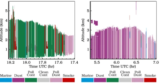
4.3 Example: dust mixture

Figure 4 shows the CALIOP and HSRL-1 aerosol type masks for a nighttime scene in the Caribbean Sea on 26 August 2010. Saharan dust is present above the ma-rine boundary layer and to some extent mixing into the boundary layer, having ad-15

vected across the Atlantic Ocean. Backtrajectory analysis (not shown) using the on-line HYSPLIT tool from NOAA Air Resources (http://ready.arl.noaa.gov/HYSPLIT.php) (Draxler and Rolph, 2013) is consistent with the transport of Saharan dust to this lo-cation. The shapes and locations of the detected aerosol layers agree very well in the CALIOP and HSRL-1 observations, and the inferred aerosol types also agree, in that 20

both systems indicate marine aerosol in the lower layer and a dust mixture with some pure dust in the upper layer. For both the CALIOP and HSRL-1 measurements, the identification of a dust mixture is based primarily on measurements of non-zero de-polarization in the scene that is nevertheless not strong enough to indicate pure dust. The dust in such a mixture dominates the lidar measurements that are used in the 25

(17)

AMTD

6, 1815–1858, 2013

S. P. Burton et al.

Title Page

Tables Figures

◭ ◮

Back Close

Full Screen / Esc

Discussion

P

a

per

|

Dis

cussion

P

a

per

|

Discussion

P

a

per

|

Discussio

n

P

a

per

|

CALIOP to distinguish the non-dust component of such a mix; however, the CALIOP algorithm demands an assumption about the non-dust component in order to model the lidar ratio. Therefore, CALIOP’s dust mixture model, polluted dust, is designed as a mixture of dust and smoke or dust and pollution and has a relatively large lidar ratio of 55 sr for version 3.01. The median HSRL-1-measured lidar ratio for this scene is much 5

lower, 35 sr, indicating that a combination of dust plus marine aerosol would be a better choice for this scene.

4.4 Example: layer boundaries and layers with multiple types

Figure 5 illustrates another scene showing advected Saharan dust in the Caribbean, two days earlier on 24 August 2010. Again, CALIOP and HSRL-1 agree well on the 10

overall shape of the detected aerosol layer and on its broad composition comprising marine aerosol, pure dust and a dust mixture. In contrast to the previous scene, how-ever, the CALIOP aerosol classification mask for this scene does not show a clear distinction at the top of the boundary layer between the marine aerosol below and the dusty aerosol above. While a primary advantage of CALIPSO observations compared 15

to passive satellites is its ability to make vertically resolved measurements of aerosol layer heights and vertical profiles of aerosol optical properties, detection of boundaries between aerosol layers of di_fferent types that are in contact with no clear air between them is a challenge. In the CALIOP algorithm, layer boundaries for contiguous aerosol layers are defined solely by changes in aerosol backscatter intensity as layers are 20

detected at successively coarser averaging resolutions in the multi-resolution layer de-tection algorithm (Vaughan et al., 2009). While aerosols of di_fferent origin may indeed differ in backscatter intensity, this is a less reliable guide to aerosol layer boundaries than intensive parameters like measured lidar ratio (from HSRL-1) or depolarization (in the case of layers containing some dust). Therefore, it is possible for a single layer iden-25

(18)

AMTD

6, 1815–1858, 2013

S. P. Burton et al.

Title Page

Tables Figures

◭ ◮

Back Close

Full Screen / Esc

Discussion

P

a

per

|

Dis

cussion

P

a

per

|

Discussion

P

a

per

|

Discussio

n

P

a

per

|

To better understand how often these multi-type layers occur, we re-examined the HSRL-1 aerosol classification results within layers. In the 109 coincident flights, a single HSRL-1 aerosol type accounts for 90 % of the AOT (as measured by HSRL-1) in only 26 % of the CALIPSO layers (the 90 % AOT threshold is used since there is some noise in the HSRL classification). Two aerosol types are required to account for 90 % of the 5

AOT in 35 % of layers, 3 aerosol types in 27 % of layers, and more than 3 aerosol types in 12 % of the layers in this comparison. The fraction of layers comprising more than one type is fairly consistent across CALIOP types, ranging from 57 % to 86 % for the six CALIOP types. Table 2 breaks down these cases according to which two HSRL-1 types contribute the most. Twenty-four percent of CALIOP marine layers in 10

this comparison contain aerosol that HSRL-1 characterizes as a dusty mix (13 %) or a combination of marine and dusty mix (11 %). Likewise, 11 % of the CALIOP desert dust layers and 14 % of the CALIOP polluted dust layers are characterized by HSRL-1 as a combination of dusty mix and marine aerosol. The 24 August 2010 case study shown in Fig. 5, where the boundary between the marine layer and the overlying dust 15

layer is not well characterized, is reflected in these numbers.

According to Table 2, a significant fraction of other CALIOP layers that are modeled as pure marine are comprised of combinations of aerosols that HSRL-1 describes as marine plus polluted marine (22 %) or marine plus urban (10 %). This finding supports the discussion of Oo and Holz (2011) and Schuster et al. (2012) who indicate that 20

CALIOP marine layers can be contaminated by pollution.

4.5 Example: overuse of polluted dust and desert dust

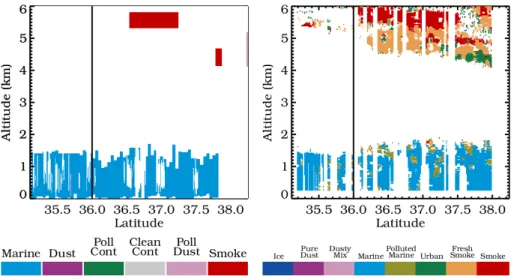
The final example illustrates a contrasting case, in which the CALIOP aerosol type mask indicates a wider variety of types than the HSRL-1 classification. Figure 6 shows a scene near Washington DC on 4 August 2007. On this day, during the CALIPSO and 25

(19)

AMTD

6, 1815–1858, 2013

S. P. Burton et al.

Title Page

Tables Figures

◭ ◮

Back Close

Full Screen / Esc

Discussion

P

a

per

|

Dis

cussion

P

a

per

|

Discussion

P

a

per

|

Discussio

n

P

a

per

|

of the layer), in agreement with a discussion of the same case study by Kacenelen-bogen et al. (2011). In contrast, the CALIOP aerosol type mask is less homogeneous and includes significant regions of polluted dust and pure dust in addition to pollution and smoke. The distinct boundaries between aerosol types in the CALIOP aerosol type mask are reflected in discontinuities in the lidar ratio and retrieved products. A similar 5

e_ffect was noted by Campbell et al. (2012) as a discontinuity in aerosol optical depth at the coastline, a statistical effect caused by the fact that certain aerosol types are limited to either land or water. However, as illustrated by Fig. 6, discontinuities between types are also present at the scale of a single CALIOP data scene.

The smoke and polluted continental aerosol types present in this scene are consis-10

tent with the types observed by HSRL-1. However, the polluted dust and desert dust are less appropriate. The HSRL-1 measured aerosol depolarization does not exceed 15 % for this scene and is therefore inconsistent with HSRL-1 observations of dust and dust mixtures; however, the CALIOP aerosol type mask indicates both polluted dust and pure dust in this scene. Part of this is explained by lower depolarization thresholds 15

for pure dust and polluted dust in the CALIOP typing scheme, 20 % and 7.5 % respec-tively (Omar et al., 2009). The higher effective aerosol depolarization threshold for dust mixtures in HSRL is related to measurement samples where the type is known, includ-ing smoke observations from a plume identified visually from the cockpit with aerosol depolarization of approximately 10 %; this suggests that the lower CALIOP threshold 20

may be too low. Yet, some of the desert dust and polluted dust layers in this scene have smaller reported aerosol depolarization values than even these lower thresh-olds. Specifically, in the lower layers, those with layer tops below about 1300 m, the reported layer-averaged particle depolarization in the CALIOP product files are below the thresholds for the assigned type. According to the CALIOP aerosol layer product, 25

(20)

AMTD

6, 1815–1858, 2013

S. P. Burton et al.

Title Page

Tables Figures

◭ ◮

Back Close

Full Screen / Esc

Discussion

P

a

per

|

Dis

cussion

P

a

per

|

Discussion

P

a

per

|

Discussio

n

P

a

per

|

To understand this discrepancy, it’s important to realize that while CALIOP’s mea-surement of volume depolarization is highly reliable (Liu et al., 2012), the depolariza-tion value used in the aerosol type identificadepolariza-tion is an estimate, an intermediate product which is affected by attenuation, sometimes dramatically. Omar et al. (2009) detail how the volume depolarization is corrected for molecular depolarization to produce an es-5

timated aerosol depolarization as part of the aerosol classification algorithm using the following equation.

δ_pest₌δv[(R−1) (1+δm)+1]−δm (R₋1) (1₊δ_m₎₊δ_m₋δ_v

whereδ_v _{indicates the volume depolarization,} δ_m _{indicates the molecular} depolariza-10

tion,δ_pestindicates the estimated aerosol depolarization, andR indicates the total scat-tering ratio (TSR), which is the ratio of the total backscatscat-tering (aerosol plus molecular) to the molecular backscattering. The total scattering ratio used in this calculation has not yet been corrected for attenuation of the laser light between the satellite and the layer being investigated. The molecular depolarization correction given by the equation 15

almost always increases depolarization over the volume depolarization value, and the contribution of the molecular correction is larger at smaller TSR values. Since attenua-tion causes the TSR to be underestimated, the aerosol depolarizaattenua-tion is overestimated and a classification of pure dust or polluted dust becomes more likely.

Figure 7 illustrates the bias towards classification of desert dust or polluted dust 20

as attenuation increases. The figure shows histograms of all V3.01 CALIOP-detected layers in the desert dust and polluted dust categories for the month of August 2006 over the continental United States. The histograms are shown as a function of parti-cle depolarization, segregated into two categories with differing amounts of overlying attenuated backscatter. Here, the particle depolarization, obtained from the CALIOP 25

(21)

AMTD

6, 1815–1858, 2013

S. P. Burton et al.

Title Page

Tables Figures

◭ ◮

Back Close

Full Screen / Esc

Discussion

P

a

per

|

Dis

cussion

P

a

per

|

Discussion

P

a

per

|

Discussio

n

P

a

per

|

dust is centered near 19–23 %. However, when there is significant attenuation (bottom panels), the distributions shift towards smaller aerosol depolarization. In the presence of a large amount of attenuation, classification of some layers as polluted dust and desert dust occurs when the aerosol depolarization is extremely small, just a fraction of a percent, due to its being overestimated in the aerosol classification stage.

5

The estimated particle depolarization could be improved by correcting the TSR for at-tenuation. While it is not possible to correct for attenuation caused by upper parts of the layer under consideration (since this calculation is done before the extinction retrieval for a given aerosol layer), much of the attenuation a_ffecting TSR is from layers above the current layer. Since the extinction retrieval for upper layers is already complete, 10

attenuation by overlying layers should be corrected and will be corrected in Version 4 of the Level 2 retrieval algorithms. Recall that the scene illustrated in Fig. 6 has quite significant aerosol loading (AOT=0.8–1.0) and it is only the lower layers that are “mis-classified” according to the CALIOP depolarization thresholds; therefore, correcting for attenuation by overlying layers is expected to fix much of the bias. It’s important to note 15

that this attenuation bias is only relevant to the aerosol classification, since attenuation is taken into account in the final aerosol depolarization product.

5 Hybrid HSRL+CALIPSO experiment

Since the HSRL-1 instrument is analogous to CALIOP but with additional channels, the coincident measurements by the airborne HSRL-1 present a unique opportunity 20

to investigate a more direct comparison between the aerosol classification algorithms themselves, operating on identical data. Using a similar strategy to Burton et al. (2010), we use only the parallel and perpendicular total backscattering signals which HSRL-1 has in common with CALIOP and do not use the molecular channel or the 1064 nm de-polarization ratio. For this comparison, measurements of attenuated backscatter from 25

(22)

AMTD

6, 1815–1858, 2013

S. P. Burton et al.

Title Page

Tables Figures

◭ ◮

Back Close

Full Screen / Esc

Discussion

P

a

per

|

Dis

cussion

P

a

per

|

Discussion

P

a

per

|

Discussio

n

P

a

per

|

combination of data measured by HSRL-1 and retrieved using CALIOP algorithms as the “hybrid HSRL-CALIOP” retrieval.

The agreement from the hybrid HSRL-CALIOP retrieval compared to the HSRL-1 aerosol classification increases for some types and decreases for others, with respect to the previous comparison between CALIOP v3.01 and HSRL-1. Specifically, the best 5

agreement is now in the polluted continental category. A large majority, 72 %, of the layers identified as polluted continental by the hybrid system are dominated by the HSRL-1 urban type, which is greater agreement than the 54 % seen in the compar-ison of CALIOP and HSRL-1 classifications. Agreement in the smoke category also improves dramatically; 57 % of the layers that the hybrid identifies as smoke are pre-10

dominately smoke or fresh smoke in the HSRL-1 classification (up from only 13 %). On the other hand, agreement for the dust and marine categories decreases. Only 69 % of the hybrid desert dust layers are considered dust or dusty mix in the HSRL-1 clas-sification results (compared to 80 % for the comparison of the CALIOP and HSRL-1 classification results) and only 43 % (compared to 62 %) of the layers identified by the 15

hybrid as marine are dominated by marine in the HSRL-1 classification. For polluted dust layers, the comparison is still poor, with only 32 % of polluted dust layers in the hybrid retrievals characterized as dusty mix in the HSRL-1 classification scheme.

Although there is increased agreement in some categories, it is perhaps surprising that using the HSRL-1 data as input to both algorithms does not result in more uniform 20

improvement in all categories. Recall that this experiment is a direct comparison of the two aerosol classification algorithms, both operating on the same underlying data, and so might be expected to produce excellent agreement in all categories. In fact, the airborne HSRL-1 measurements have a higher signal-to-noise ratio than the CALIOP measurements, and might be expected to improve the classification for that reason. 25

(23)

AMTD

6, 1815–1858, 2013

S. P. Burton et al.

Title Page

Tables Figures

◭ ◮

Back Close

Full Screen / Esc

Discussion

P

a

per

|

Dis

cussion

P

a

per

|

Discussion

P

a

per

|

Discussio

n

P

a

per

|

in Sect. 4.4, not changes in aerosol type. Re-examination of two of the above examples will serve to explain how this a_ffects the type comparison.

Figure 8 shows the aerosol classification mask from the hybrid measurements com-prised of Level-1-like data measured by HSRL-1 and retrieved via the CALIOP algo-rithms, for the 4 August 2007 and 24 August 2010 cases (the same scenes shown 5

in Figs. 6 and 5, respectively). The classification in the 2007 Washington DC case is improved compared to Fig. 6, for now most of the scene is identified as polluted con-tinental, in good agreement with the identification of urban aerosol from the HSRL-1 classification. In contrast, the classification for the 2010 Caribbean case is less accu-rate than the CALIOP classification shown in Fig. 5, as now almost none of the aerosol 10

is identified as marine. An obvious feature of the aerosol classification masks from the hybrid retrieval in both cases is the fact that most of the identified aerosol layers extend all the way from the highest altitude where aerosol is detected down to the surface; in other words, there are almost no internal boundaries between types. The reason for this is that the higher signal-to-noise ratio from HSRL-1 allowed the CALIOP retrieval 15

algorithm to detect most of the aerosol layers at the smallest averaging resolution, 5 km. In fact, the CALIOP detection algorithm is quite robust and accurately detects very ten-uous aerosol layers in the data. However, since all the aerosol in Fig. 8 is detected in a single pass through the CALIOP multi-averaging detection scheme, each column includes only a single layer, and that layer is assigned a single type by the algorithm. 20

This e_ffect explains both the better agreement between the hybrid HSRL-CALIOP sys-tem and HSRL-1 observations for the Washington DC case and the worse agreement in the Caribbean case. In both cases, since only a single layer is detected, the ob-served aerosol depolarization is averaged over the entire height of the aerosol column. Therefore, the layer-averaged aerosol depolarization in the pollution case drops below 25

(24)

AMTD

6, 1815–1858, 2013

S. P. Burton et al.

Title Page

Tables Figures

◭ ◮

Back Close

Full Screen / Esc

Discussion

P

a

per

|

Dis

cussion

P

a

per

|

Discussion

P

a

per

|

Discussio

n

P

a

per

|

in the same column in the CALIOP classification are effectively combined together in the hybrid retrieval into single-layer columns of pure dust or polluted dust. It is important to note that the multi-resolution layer detection algorithm of CALIOP is well designed for the lower signal-to-noise observations of the satellite instrument, so the lack of in-ternal layer boundaries in the hybrid experiment should not be taken to indicate a flaw 5

in the CALIOP algorithms. However, this result illustrates how the CALIOP scheme can fail to identify different aerosol types within a single column, since internal bound-aries between aerosol types in the CALIOP products are primarily related to changes in backscatter intensity rather than aerosol intensive parameters that are directly linked to aerosol type. The relatively poor agreement in some categories, in common with 10

the original comparison, also reinforces that it is not primarily the increased signal-to-noise ratio that allows for more accurate aerosol classification from the HSRL-1 measurements, but the increased information content, in the form of aerosol intensive parameters that give direct insight into aerosol type.

6 Summary and discussion

15

In this study, we have compared the aerosol classification products from CALIOP with those from the NASA Langley airborne HSRL-1 instrument. The HSRL-1 aerosol clas-sification makes use of four aerosol intensive properties that depend only on aerosol type and not amount to classify each range-resolved measurement. The CALIOP aerosol classification strategy is necessarily di_fferent, since aerosol type is a required 20

input for the extinction retrieval. The CALIOP typing uses an estimate of aerosol de-polarization, attenuated backscatter, layer height, and location information. It is done on integrated layers that are detected by a separate algorithm that is not designed to detect di_fferences in aerosol type. For this comparison, all aerosol layers on 109 un-derflights of the CALIOP orbit track were examined, showing best agreement for desert 25

(25)

AMTD

6, 1815–1858, 2013

S. P. Burton et al.

Title Page

Tables Figures

◭ ◮

Back Close

Full Screen / Esc

Discussion

P

a

per

|

Dis

cussion

P

a

per

|

Discussion

P

a

per

|

Discussio

n

P

a

per

|

case studies which yielded specific insights which could potentially lead to incremental improvements in the CALIOP aerosol classification product.

First, we find that the CALIOP polluted dust category includes not just the cases of dust mixed with pollution or smoke for which it was designed, but also cases where dust is mixed with marine aerosol. An improvement to the inferred lidar ratio for dust mixtures 5

would be possible if the typing algorithm were refined to distinguish between di_fferent dust mixtures, specifically between mixtures of dust plus pollution or smoke, which would have a lidar ratio greater than pure dust, and mixtures of dust plus marine, which would have a lidar ratio less than pure dust. It may be possible to separate di_fferent dust mixtures in the CALIOP retrieval by adding the attenuated backscatter color ratio to the 10

information that is used for diagnosing aerosol type. Although the color ratio from the attenuated backscatter (i.e., Level 1 data) is not the same as the true backscatter color ratio (which depends on selection of the lidar ratios), the work of Oo and Holz (2011) on cases over water (without dust) suggests that CALIOP’s attenuated backscatter color ratio may be su_fficient to distinguish marine aerosol from smoke aerosol. Research 15

is ongoing as to whether there is sufficient particle-size information in the attenuated backscatter color ratio to distinguish mixtures of dust and marine from mixtures of dust and smoke or pollution.

Second, we find that the polluted dust and desert dust types are found more fre-quently in CALIOP data than in HSRL-1 data for two reasons. The first is smaller 20

thresholds on depolarization for these types in the CALIOP algorithm compared to the HSRL-1 aerosol typing algorithm. The second and more important reason is an attenuation-related depolarization bias. A correction for attenuation should be included in the estimated aerosol depolarization that is used in the classification. In fact, the CALIOP team plans to correct for attenuation in overlying layers in the version 4.0 re-25

(26)

AMTD

6, 1815–1858, 2013

S. P. Burton et al.

Title Page

Tables Figures

◭ ◮

Back Close

Full Screen / Esc

Discussion

P

a

per

|

Dis

cussion

P

a

per

|

Discussion

P

a

per

|

Discussio

n

P

a

per

|

Our final finding is that the reported layer heights of contiguous aerosol layers of dif-ferent types do not accurately reflect the boundaries between di_fferent aerosol types. The detection algorithm is not designed to separate aerosol by type and can fail to identify different aerosol types within a column. Rather, internal boundaries between aerosol types in the CALIOP layers are related only to detection resolution. In specific 5

cases like the Caribbean example studied here, where two aerosol types with diff er-ing amounts of depolarization occur in contiguous layers, CALIOP theoretically has the information content to separate them. It may be profitable to use the CALIOP depolar-ization measurements to refine the detected layer boundaries in such cases.

As stated above, the primary role of the aerosol classification in the CALIOP al-10

gorithms is to enable an accurate inference of the lidar ratio for use in the retrieval of aerosol extinction and backscatter profiles. However, the combination of qualitative knowledge of the aerosol type with accurate quantitative profile measurements has other useful applications, including model assessment and improvement, and air qual-ity detection and management. Based on our results, a future satellite lidar similar to 15

CALIOP, but with the addition of polarization sensitivity at 1064 nm and the HSRL tech-nique at 532 nm could provide a significant advancement in characterizing the vertical distribution of aerosol for climate and air quality applications.

Recently, LaRC has built and deployed a follow-on instrument, HSRL-2, the first airborne multi-wavelength HSRL instrument, with HSRL capabilities at both 355 and 20

532 nm (http://fallmeeting.agu.org/2012/files/2012/12/A13K-0336 Hostetler et al.pdf). It also uses the standard backscatter technique at 1064 nm and measures depolar-ization at all three channels. This combination of measurements provides additional in-formation content and is expected to provide aerosol classification improvements over the HSRL-1 classification studied here.

25

(27)

AMTD

6, 1815–1858, 2013

S. P. Burton et al.

Title Page

Tables Figures

◭ ◮

Back Close

Full Screen / Esc

Discussion

P

a

per

|

Dis

cussion

P

a

per

|

Discussion

P

a

per

|

Discussio

n

P

a

per

|

No. DE-AI02-05ER63985. The authors also acknowledge the NOAA Air Resources Laboratory (ARL) for the provision of the HYSPLIT transport and dispersion model and READY website (http://www.arl.noaa.gov/ready.php) used for some of the analysis described in this presen-tation. The authors would also like to thank the NASA Langley B200 King Air flight crew for their outstanding work in support of HSRL measurements, the engineering team who work 5

untiringly on building and maintaining excellent HSRL instruments, and our colleagues who operated HSRL-1 in flight and processed the measurements.

References

Alados-Arboledas, L., M üller, D., Guerrero-Rascado, J. L., Navas-Guzm án, F., P érez-Ram´ırez, D., and Olmo, F. J.: Optical and microphysical properties of fresh biomass burn-10

ing aerosol retrieved by Raman lidar, and star-and sun-photometry, Geophys. Res. Lett., 38, L01807, doi:10.1029/2010gl045999, 2011.

Amiridis, V., Balis, D. S., Giannakaki, E., Stohl, A., Kazadzis, S., Koukouli, M. E., and Zanis, P.: Optical characteristics of biomass burning aerosols over Southeastern Europe determined from UV-Raman lidar measurements, Atmos. Chem. Phys., 9, 2431–2440, doi:10.5194/acp-15

9-2431-2009, 2009.

Burton, S. P., Ferrare, R. A., Hostetler, C. A., Hair, J. W., Kittaka, C., Vaughan, M. A., Ob-land, M. D., Rogers, R. R., Cook, A. L., Harper, D. B., and Remer, L. A.: Using airborne high spectral resolution lidar data to evaluate combined active plus passive retrievals of aerosol extinction profiles, J. Geophys. Res.-Atmos., 115, D00H15, doi:10.1029/2009jd012130, 20

2010.

Burton, S. P., Ferrare, R. A., Hostetler, C. A., Hair, J. W., Rogers, R. R., Obland, M. D., But-ler, C. F., Cook, A. L., Harper, D. B., and Froyd, K. D.: Aerosol classification using airborne High Spectral Resolution Lidar measurements – methodology and examples, Atmos. Meas. Tech., 5, 73–98, doi:10.5194/amt-5-73-2012, 2012.

25

Campbell, J. R., Reid, J. S., Westphal, D. L., Jianglong, Z., Hyer, E. J., and Welton, E. J.: CALIOP aerosol subset processing for global aerosol transport model data assimilation, IEEE J. Sel. Top. Appl., 3, 203–214, doi:10.1109/jstars.2010.2044868, 2010.