en 0104 530X gp 0104 530X1874 14

http://dx.doi.org/10.1590/0104-530X1874-14

Resumo: Linhas de montagem mista combinam a fabricação de diferentes modelos de produtos em uma única linha de montagem, proporcionando lexibilidade de produção de acordo com a sazonalidade de vendas, evitando a baixa utilização dos ativos. Este artigo propõe uma heurística para balanceamento em linhas de produção sujeitas a distintos mix de produtos com vistas a atenuar as restrições de capacidade nas estações de trabalho e aumentar a eiciência de balanceamento. A abordagem proposta foi aplicada em uma linha de montagem mista com 7 modelos de produtos. Os resultados foram considerados satisfatórios, segundo avaliação de especialistas, quando avaliados em termos de capacidade produtiva, ciclo de fabricação e balanceamento de linha.

Palavras-chave: Linha de montagem mista; Balanceamento; Capacidade; RPW.

Abstract: A mixed-model assembly line can manufacture different products in the same assembly line, providing lexible production according to demand seasonal behavior. This article proposes a heuristic that aims to balance production lines subjected to several product models in order to attenuate capacity restrictions in workstations and increase the balancing eficiency. The proposed approach was applied to a mixed assembly line composed of seven product models. The results were considered satisfactory when assessed in terms of production capacity, manufacturing cycle time, and assembly line balancing.

Keywords: Mixed-model assembly line; Line balance; Capacity; RPW.

Mixed assembly line balancing method in scenarios

with different mix of products

Balanceamento de linha de montagem mista em cenários com distintos mix de produtos

Gustavo Reginato1

Michel José Anzanello1

Alessandro Kahmann1

Lucas Schmidt1

1 Departamento de Engenharia de Produção e Transportes, Universidade Federal do Rio Grande do Sul – UFRGS, CEP 90040-060, Porto Alegre, RS, Brazil, e-mail: reginato205@yahoo.com.br; anzanello@producao.ufrgs.br; alessandro.kahmann@ufrgs.br; lucasximiti@hotmail.com Received Nov. 14, 2014 - Accepted May 5, 2015

Financial support: None.

1 Introduction

Recent trends in customer demand for customized products encouraged the implementation of mixed assembly lines in many industrial environments (Mendes et al., 2005). Mixed lines can produce more than one kind of product in the same assembly line (AL) (Becker & Scholl, 2006), and different sales cycles may be combined to avoid low asset utilization when low sale of a speciic product occurs (Leone & Rahn, 2004). However, in order to mixed arrangements to become viable in high competitive markets, assembly lines designers seek to increase the eficiency by maximizing the income rate and minimizing operating costs. Therefore, the assembly lines project an issue of great industrial interest (Rekiek et al., 2002a).

Aspects of balancing, layout and requested product mix affect the performance of a joint assembly line. The product mix is the quantity of each product

being manufactured by AL. However, the lack of parts, machinery and equipment unavailability and non-conformities parts, among others, restrict the production of certain models in certain periods. In such way, changes in mix production are required to ensure that available resources are used. Such utilization, however, typically proves dificult to be carried out as the capacity constraints, imposed by balancing, limit the production rate. Thus, whether AL have conditions to adapt themselves to different product mix without affecting the productive capacity, the use of available resources can be maintained.

precedence diagram; (ii) allocate tasks to a workstation until the total station weighted average time does not exceed the moving target, and (iii) allocate tasks to a workstation in a way the total time does not exceed the station cycle time. The proposed method was applied in a company presenting a mixed AL that produces 7 different models. The method increased the production capacity by 35% (meeting the required demand for the AL), reduced the products crossing time in AL and improved line eficiency and balancing due to a better distribution of tasks.

This paper is divided into ive sections. Section 2 presents the literature review, detailing the assembly line types, its balancing and applicable solutions. Section 3 presents the method stages, and its application in the production environment is in Section 4. Section 5 brings the conclusions.

2 Theoretical background

An AL consists of a production arrangement formed by workstations typically distributed over a movement system. The product is sequentially released from station to station, suffering changes until it reaches the inal assembly station (Gerhardt, 2005; Becker & Scholl, 2006; Kriengkorakot & Pianthong, 2007).

The assembly lines that produce identical products are call single-model line, or one-model line. When there are differences in the products, two classiications arise. The irst is the multi-model line or multi-line model, which shows signiicant differences in production processes, and different products are manufactured in larger batches than a unit to minimize the setup impacts. The second classification is known as mixed-model line or mixed line, which is apply when there is similarity of productive process and there is no setup for process adjustment. This makes it possible to launch the products in the line in units randomly (Smiderle et al., 1997; Becker & Scholl, 2006). For each model, different processing times are required, so the amount of work at the same operator in the same workstation is uneven. Cases which operator ends the job before the next cycle or not ends the job within the cycle time make AL unbalanced and eficiency is reduced (Sarker & Pan, 1998). Even so, for Askin & Standridge (1993) apud Souza et al. (2003), this production system tends to be one of the most eficient, but requires reliable process and it with low variability in processing time of the workstations (in the practical application context of the methodology proposed, low variability refers to a difference less than 30% of the time variation between models). Figure 1 illustrates the above deinitions, where the geometry of the igures refers to different products.

workstations; (iii) balance the AL; and (iv) determine

the models production order. Another concern of AL design is to minimize the lead time (Sarker & Pan, 1998), which means reducing the gap of time between the initiation and completion of the product AL (Marlin, 1986). As shorter is the lead time, greater the potential sale of products (Öztürk et al., 2006). Another premise for the proper functioning of ALs is time the station (S) does not exceed the cycle time,

according to Equation 1.

1 maxt_k maxS_j T_c

D

≤ ≤ ≤ (1)

where S_j is the total time of station j (j=1,...,W), representing the sum of performing times tasks allocated to each station in time units; t_k is the processing time of the kth _{task on time unit; k} identiies the task

such that k=1,..., N; T_c is the time cycle and D is the product demand rate.

The cycle time (T_c) is the time when a product

is released from station to station, deined by the Equation 2.

c

availabletimein period p

T

demand in period p

= (2)

The number of workstations needed to meet demand varies with the AL settings and restrictions. According Peinado and Graeml (2007), the minimum number of workstations for ALs counting with only one operator can be estimated by Equation 3.

c

individual taskstimes

Number of workstations

T

=

∑

To balance the tasks, it is essential to know precedence diagram (Figure 2). This diagram shows the order of tasks execution, respecting technological requirements or item production characteristics (Boysen et al., 2007).

In precedence diagram, the numbers within the circles represent tasks, while the arrows joining the circles show the precedence relation. The sum of

Figure 1. Assembly line types. Source: Adapted from

the tasks times assigned to a station is known as station time.

Each task time can be achieved by chrono-analyse among other methods. The chrono-analyse is a way of measuring the work by means of statistical methods, allowing calculating the standard time. The standard time includes a series of factors, such as operator speed, personal needs and relieving fatigue, among others; such factors can be found in specialized literature in the area. The standard time of performing tasks can also be determined by predetermined times (Peinado & Graeml, 2007).

The task processing times are also used to determine the production capability of a AL. Capacity is the maximum amount of items produced in the AL in a given time interval; to determine the production capacity, it is necessary to identify the bottlenecks in the AL. Therefore, the production capacity is calculated on the basis of working time available and the time of the bottleneck station, as in Equation 4 (Peinado & Graeml, 2007).

Availabletimein period p

Production capacity

Time of thebottleck station

= (4)

2.2 Assembly line balancing

The Assembly Line Balance (ALB) is known as the classic problem of AL balancing, consisting in the allocation of tasks on a workstation in a way that downtime is minimized and the precedence constraints are met (Rekiek et al., 2002b; Becker & Scholl, 2006; Kriengkorakot & Pianthong, 2007). The ALB allows achieve the best use of available resources so that satisfactory production rates are reached at a minimum cost (Wild, 1972, apud Praça, 1996). The balancing is necessary when there are process changes, such as adding or deleting tasks, change of components, changes in processing time (Farnes & Pereira, 2006) and also in the implementation of new processes.

According to Becker & Scholl, 2006, the assembly line balancing problem can be classiied into four categories, as shown in Figure 3. This classiication is detailed as follows:

(i) DSM – Deterministic single model: This model is considered to assembly lines with only one product model, where the tasks times are known deterministically, with little tasks timing variation (as a result of easy execution and also the operators motivation) (Rekiek et al., 2002a; Becker & Scholl, 2006). Certain eficiency criteria should be otimizated, as idle time station and line eficiency, among others; (ii)

SSM – Stocastic single model: In this category, the execution times of activities have resulting human behavior variability, inability of operators, lack of motivation, complex processes and equipment with low reliability, among others; (iii) DMM - Deterministic multi/mixed model:

The formulation of the DMM problems considers deterministic tasks times, but with the presence of different products manufactured on the same assembly line. In this context, aspects associated with sequencing, release rate and batch sizes become important when compared to single model lines; and (iv) SMM - Stocastic multi/ mixed model: the tasks times are probabilistic. Learning impacts, skill, tasks delineation and tasks time variation are considered in this approach (Becker & Scholl, 2006).

Another important classiication split the line balancing problems into two categories: (i) simple assembly line balancing problems, indicating that no restrictions are relaxed; and (ii) generic balancing

problems, which it the line balancing problems

that aim to solve problems with additional features (Fernandes et al., 2008).

According Van Zante-de Forkket & De Kok (1997) apud Gerhardt (2005), the fundamental difference between a single model line balancing problem for a multi-model is the precedence diagram. Such, many authors, to develop methods to solve multi-model line balancing problems, transform the problem into single model. Two methods can be used: (i) equivalent precedence diagram, and (ii) adjusting the processing

taks time (Gerhardt, 2005).

(i) Equivalent precedence diagramming method: Thomopoulos (1970) apud Gerhardt

(2005) assumed that in a mixed line, there are several common tasks to the various models produced and, consequently, a similar set of precedence relationships. Then, the precedence diagrams combination of each individual model can be made by joining the nodes and precedence relations of the respective diagrams for each model, as exempliied by the Figures 4 and 5. According to van Zante-de Fokkert & de Kok (1997), the balance of AL multi-model based on equivalent precedence diagramming method can be compared to balancing single AL model. However, the allocation of tasks to workstations is performed based on the total shift time duration and not in cycle time, which is used as the basis to balancing AL single model.

(ii) Setting task processing time method: In this method, the processing time is determined by the weighted average of kth _{task common to}

different models, according to the Equation 5 (van Zante-de Fokkert & de Kok, 1997),

, 1

M

k m k m m t pd t

=

=

∑

Figure 3. AL balancing problem classiication. Source: Adapted from Ghosh & Gagnon (1991).

Figure 4. Precedence diagram to the model A (a) and model

where pd_m is the proportion of the model m ahead the other models produced in AL, t_k,m represents the processing time for the kth _{common task for}

different models and tk represents the processing time weighted average of the kth _{common task to}

different models. An advantage of this method is that it is based on the cycle time, which makes more sense for organizing tasks in a AL (instead using it total shift time). As disadvantages, the method does not determine the sequence in which the models will be produced and does not consider different diagrams of precedence. As such, it is recommended for balancing derivatives models of a basic model, where the tasks have a processing time similar to the basic model (van Zante-de Fokkert & de Kok, 1997).

In turn, Becker & Scholl (2006) emphasizes that both methods (i) and (ii) exhibit ineficiencies resulting from variations in stations processing times, which depend on the production model. Such inconsistencies may generate work overload or idle for operators.

Traditionally, two indicators are used to evaluate balancing quality AL (Driscoll & Thilakawardana, 2001): Balance Delay, which represents a percentage of time that the AL remains idle; and Smoothness Index (softness Index), which measures the difference between the maximum total working time between the stations and the total times of the other work stations (Gerhardt, 2005).

Driscoll & Thilakawardana (2001) introduce alternative ways to evaluate the balance of the AL. The Line eficiency (LE) quantiies the use of AL and has aspects of economic evaluation; Balancing eficiency (BE) quantiies the tasks allocation quality for the workstations, which may consequently cause an increase in the production rate. Both indicators are dimensionless and represented using a scale from

0 to 100%, where 100% represents the best result. They are calculated according to Equations 6 and 7 respectively. 1 ₁₀₀ N k k c t LE W T =

=

∑

1 1 100 W j av j av S S BE W S =  ₋    =_{ ×} − _ ×    

∑

where S_av is the average time of workstations and W

the number of workstations.

2.3 Soluctions for ALB

Considering that the ALB problem may be shown on NP-hard combinatorial optimization category, several researches have developed computational or heuristic approaches (Ghosh & Gagnon, 1991). Ghosh & Gagnon (1991) classify methods for balancing ALB as follows: (i) Rank and Assign Methods: In these methods, tasks are sorted based on criteria or rules of priority and assigned to stations relying on an order that does not violate the relationship of precedence constraints and cycle time; (ii) Tree Search Methods: These methods are essentially integer programming relying on the Branch & Bound method. Approaches in this category can also be termed as enumerative methods; (iii) Random Sampling Methods: These methods randomly assign tasks to workstations in view of the precedence constraint and cycle time; and (iv) Other methods: aggregation methods (task elements are grouped into composite tasks), Successive Approximation (a great algorithm is applied successively as a heuristic in a simpler version of the problem), and Learning Methods (based on the premise that the experience acquired minor problem solving is used to solve larger problems).

Cristo (2010), Ponnambalam et al. (1999) and Chow (1990) highlight the following heuristics to ALB troubleshooting: Rank positional weight, Kilbridge and Wester’s method, Largest set ruler. The foundations of heuristics above are now displayed.

• RPW-Rank Positional Weight: this method was introduced by Hegelson and Birnie in the 60s, having generated satisfactory and fast solutions according Boctor (1995) apud Praça (1996). Its operation consists in calculating the positional weight of each task according to the precedence diagram. The weight is the sum of the task time with the time tasks that predate it. In sequence, the positional weights should be arranged in descending order, and the tasks assigned to the workstations according to the order of the positional weight, respecting the Figure 5. Precedence diagram equivalent models A and B.

precedence constraints. Further details on the method can be found in Chow (1990). • Kilbridge e Wester Method (KWM): This

method selection work elements to describe the station according to the column Precedence Diagramming position as shown in Figure 6. In sequence, tasks are arranged in descending order of processing time. Finally, tasks are allocated to workstations in accordance with such order, thus ensuring that the largest elements are allocated irst and increasing the chance of each station time get closer to the cycle time (Gerhardt & Fogliatto, 2004).

• Largest Candidate Rule (LCR): This heuristic allows obtaining results in less time than the positional weights method. Initially, one should list tasks in descending order of processing time; then the task should be assigned to the workstations according to the order of the list without violating any precedence constraint or exceed the cycle time (Praça, 1996).

3 Method

This section proposes a new balancing heuristics for mixed AL titled target mobile RPW (RPW-MVM), which relies on heuristics of RPW positional weights originally proposed by Helgeson & Birnie. Such proposition focuses on a production environment amenable to changes in product mix, which cause imbalances on the workstations and generate productive capacity constraints in AL, making it unable to meet the required production demand.

The heuristic allows the AL meets the production demands characterized by several product mix composition, without the need for interventions to balancing adjustment or sequencing of actions to launch the products. This requires that the time of each model on all workstations is less than the AL cycle time. In addition, the proposed heuristic innovates in the tasks distribution format to workstations, proposing a target mobile which aims to improve the tasks distribution between the stations compared to the original RPW. The proposed heuristic is now detailed.

3.1 RPW-MVM

The original RPW is fundamentally guided by a pre-established time cycle; therefore, it can be assumed that the amount limiting target of the allocable task to a given workstation is the cycle time, which is ixed. Thus, the tasks allocation to workstations may have an accumulated imbalance in the irst workstation, which typically results in signiicant losses to the AL. It is proposed then a change in this target, which becomes mobile (and called Moving Target - MVM).

The MVM is calculated for each workstation and depends on the number of workstations to be balanced. It serves to improve the tasks distribution between the workstations not balanced according to the time of the not yet allocated tasks. Every changing of the station, the target is recalculated for each model (hence mobile), and then identiied the condition that allows allocation of the remaining tasks of the product with longer not yet allocated operations. In other words, MVM allows for each workstation to exchange the entire contents of the working model under review to be distributed evenly among the remaining stations.

Figures 7 and 8 illustrate the RPW without target mobile and with moving target (MVM), respectively.

Figure 6. Precedence diagram divided in column by Kilbridge and Wester method. Source: Adapted from Gerhardt &

The MVM yields better smoothness index for AL and, therefore, beneit and ergonomic productive character.

Following are presented the steps to perform the RPW-MVM.

Step 1: Set the diagram/equivalent precedence matrix of all models;

Step 2: Unlike the RPW in AL single model, the RPW-MVM is a balancing in a AL with more than one product model, where each model has its own tasks processing time. So for the average processing time for common tasks to the different models, is needed to deine the each model proportion to be produced by the Equation 8

m m

d pd

D

= (8)

where d_m is the product demand in the period p such that m=1,...,M; and D is the total demand for all models

for the period p. The products demand history or the

production plan are reference sources for deining the product number of the model m.

Step 3: Calculate the cycle time (Tc) based on

total production demand to be met by the Equation 2;

Step 4: As mentioned earlier, the RPW-MVM support in times of an equivalent product of mixed AL. Thus, for the tasks allocation in the RPW-MVM, use the Time Weighted Average (tk) and the weighted

average total station time (Sj ), calculated using

Equations 9 and 10, respectively.

, 1

M

k m k m m t pd t

=

=

∑

j k k j

S t

∈

=

∑

Figure 7. Balancing with RPW and without MVM heuristics. Source: The authors.

Step 5: Calculate the RPW of each task by adding

k

t to the processing times of all preceding tasks equivalent precedence diagram;

Step 6: Sort the tasks in descending order of RPW; Step 7: Calculate the minimum number of workstations for balancing ALM (MinW) and then set the last workstation (W=MinW) based on the Equations 11 and 12, where CTTm is the total workload the m model.

, 1

N

m k m k CTT t

=

=

∑

Min , 1,m

c CTT

W m M

T

= = … (12)

Step 8: Set j W= ;

Step 9: Calculate the moving target of the latest workstation for all models

(

)

is required for each product model and should be recalculated every new balanced workstation during application of the RPW-MVM. The moving target the

jth _{workstation to the model m (} , )

j m

MVM ) is calculated

by Equation 13 based on the not yet allocated workload residue divided by the total workstations still unbalanced for the m model. Equation 14 sets the total charge allocated at station j of the m model (CTAj,m).

, 1, ,

j m j m j m

CTA =CTA+ +S (13)

( 1, ) ,

m j m j m CTT CTA

MVM

MinW MinW j+

−

= _{− −} (14)

Step 10: Allocate most task RPW to the station j, while respecting the precedence relation of the equivalent diagram of precedence, and the weighted average total station time [so that it does not exceed the largest MVM

(

(

)

)

pay attention to that the total time m model at the station does not exceed the cycle time ((Sj m, = …1, M≤Tc);

Step 11: Repeat the process designating the task to stations until there is no feasible task to at least one of the models;

Step 12: Set (j j= −1) e recalculate MVMj m, = …1, M;

Step 13: Validate the inequality

(

)

if met, proceed to the next step; otherwise, return to step 8, reset (MinW=MinW 1+ ) and restarting the task

allocation process; and

3.2 Balancing assessment generated by the RPW-MVM

The balancing analysis of the resulting RPW-MVM heuristic relies on static indicators, ie without the use of dynamic simulation methods. Thus, in some cases, they are calculated in the AL bottleneck position (g),

where production is limited according to Peinado & Graeml (2007). The indicators are: (i) the amount of AL workstations; (ii) capacity in the bottleneck situation (Cap_b), as depicted in Equation 15; and (iii) crossing time estimated in the bottleneck position (TCestm_b); (iv) Line Eficiency bottleneck situation (LE_b) and (v) balancing eficiency (BE).

b

g

availabletimeinthe period p

Cap

T

= (15)

Where T_g is the bottleneck processing time, deined by the major Sj= …1, W m, = …1, M.

Likewise, the crossing time estimated by the bottleneck situation (TCestimb), shown in Equation 16

also uses the bottleneck processing time in obtaining it.

( )

b g

TCestim = + ×Number of workstations A T (16)

where A is the number of products not allocated to workstations, but located between the beginning and the end of AL (eg, buffers).

Line Eficiency bottleneck situation (LEb) is calculated by Equation 17, whereas the balancing eficiency (BE) is given by Equation 18.

1 ₁₀₀ N k k b g t LE W T = = × ×

∑

1 1 100 W j av j av S S BE W S =  ₋    =_{ ×} − _ ×    

∑

4 Results and discussion

The method was applied in a AL belonging to a manufacturer of agricultural machines of the type drawn with unit manufacturing lot. The AL is organized into ive workstations; in each station there is an operator. Moreover, among the workstations there is a buffering unit that has the function of absorbing excess processing time for some models about the cycle time. Figure 9 illustrates the AL current low,

with the number of workstations within the marked blocks and buffers marked with “x” in the center. All computational procedures were performed in spreadsheet.

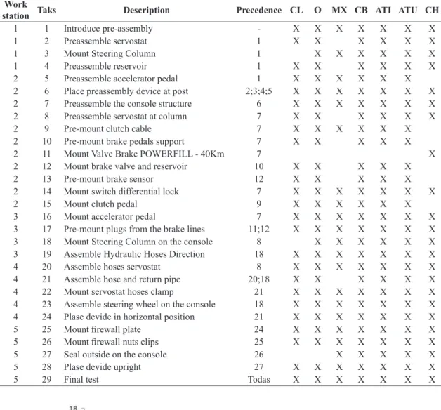
The AL in study manufactures seven models of products, called CL, O, MX, CB, ATI, ATU and CH, which are assembled through up to 29 different tasks depending on the model. Table 1 shows the

Figure 10. Actual AL balancing. Source: The authors. Table 1. Performed tasks in the AL for each model.

Work

station Taks Description Precedence CL O MX CB ATI ATU CH

1 1 Introduce pre-assembly - X X X X X X X

1 2 Preassemble servostat 1 X X X X X X

1 3 Mount Steering Column 1 X X X X X X

1 4 Preassemble reservoir 1 X X X X X X

2 5 Preassemble accelerator pedal 1 X X X X X X

2 6 Place preassembly device at post 2;3;4;5 X X X X X X X

2 7 Preassemble the console structure 6 X X X X X X X

2 8 Preassemble servostat at column 7 X X X X X X

2 9 Pre-mount clutch cable 7 X X X X X X

2 10 Pre-mount brake pedals support 7 X X X X X

2 11 Mount Valve Brake POWERFILL - 40Km 7 X

2 12 Mount brake valve and reservoir 10 X X X X X

2 13 Pre-mount brake sensor 12 X X X X X

2 14 Mount switch differential lock 7 X X X X X X X

2 15 Mount clutch pedal 9 X X X X X X

3 16 Mount accelerator pedal 7 X X X X X X X

3 17 Pre-mount plugs from the brake lines 11;12 X X X X X X X

3 18 Mount Steering Column on the console 8 X X X X X X

3 19 Assemble Hydraulic Hoses Direction 18 X X X X X X X

4 20 Assemble hoses servostat 8 X X X X X X X

4 21 Assemble hose and return pipe 20;18 X X X X X X

4 22 Mount servostat hoses clamp 21 X X X X X X X

4 23 Assemble steering wheel on the console 18 X X X X X X X

4 24 Plase devide in horizontal position 21 X X X X X X X

5 25 Mount irewall plate 24 X X X X X X X

5 26 Mount irewall nuts clips 25 X X X X X X X

5 27 Seal outside on the console 26 X X X X X

5 28 Plase devide upright 27 X X X X X X X

The current AL workload is shown in Figure 10, with the times (in minutes) per workstation and model.

The current planned demand of AL is 37 products per shift, which are thrown randomly into production (no structured sequencing). Each turn consists of 480 minutes of production time, excluding stops for meeting, lunch and breaks.

As can be seen in Figure 10, only the stations 3 and 5 have ability to 37 product/shift for any product, since the time all product models is less than the cycle time. Currently, AL capacity at bottleneck situation is 28 products per shift.

Table 2 presents the mix of products using the company’s production plan and the proportion of each model calculated from Equation 8.

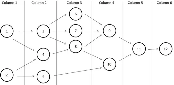
Then it was drafted precedence matrix equivalent to all models, as shown in Figure 11.

Based on the total demand of 37 products per turn, we calculated the cycle time (T_c) using Equation 2,

which resulted in 12.97 min.

Table 3 shows the time weighted average processing for each task and the RPW for each task calculated using Equation 9.

After increasingly ordering the tasks in accordance with the value of the RPW, it was determined the number of the last workstation (W). To do this, we

a worst case model with higher MinW (in this case, the ATU model, according to Table 4).

Further, steps 9 were performed by 14 of the method presented in section 3. The values of MVMj m, are shown

in Table 5; stands out in bold the value of MVMj m,

according to j allocation of tasks to workstations. The new balance of AL is shown in Figure 12, with the times per workstation and per model.

It can be seen in Figure 12, all workstations have less processing time than the cycle time. Thus, the new balancing provided the AL able to produce 37 products/turn, regardless of the proportion or type of product manufacture. A summary of the tasks allocation to the workstations is shown in Chart 1. As can be seen, there was an increase of 1 workstation

Figure 11. Equivalent precedence diagram. Source: The authors. Table 2. Deinition of the production.

PRODUCT MODEL

Τ

CL O MX CB ATI ATU CH

MIX (quantify for model) 0.8 1.2 0.4 12.5 1.7 20.0 0.4 37.0

Proportion of model 2% 3% 1% 34% 4% 54% 1% 100%

Chart 1. Tasks allocation to workstations for balancing the

AL.

Workstation Task

1 1; 2; 4; 5

2 3; 6; 7; 14

3 8; 9; 10; 12; 16; 18

4 11; 15; 20; 23

5 13; 17; 19; 21

Table 3. Weighted average processing time and tasks RPW.

Taks

PRODUCT MODEL

t_k RPW

CL O MX CB ATI ATU CH

2% 3% 1% 34% 4% 54% 1%

1 Introduce pre-assembly 0.37 0.37 0.37 0.37 0.37 0.37 0.37 0.37 0.37

2 Preassemble servostat 4.49 4.49 0.00 4.49 4.49 4.49 4.49 4.44 4.81

3 Mount Steering Column 0.00 5.59 5.59 5.59 3.40 8.77 5.59 7.08 7.44

4 Preassemble reservoir 3.50 3.50 0.00 3.50 3.50 3.50 3.50 3.46 3.82

5 Preassemble accelerator pedal 3.99 3.99 3.99 3.99 3.99 3.99 0.00 3.94 4.31 6 Place preassembly device at post 0.99 0.99 0.99 0.99 0.99 0.99 0.99 0.99 20.28 7 Preassemble the console structure 0.65 0.65 1.25 1.25 1.25 1.25 1.25 1.22 21.50 8 Preassemble servostat at column 3.42 1.47 0.00 2.29 2.29 2.29 2.29 2.26 23.77 9 Pre-mount clutch cable 0.56 0.56 0.56 0.56 0.56 0.56 0.00 0.55 22.05 10 Pre-mount brake pedals support 0.96 0.96 0.00 0.96 0.96 0.96 0.00 0.94 22.44 11 Mount Valve Brake POWERFILL - 40Km 0.00 0.00 0.00 0.00 0.00 0.00 2.08 0.02 21.53 12 Mount brake valve and reservoir 2.08 2.08 0.00 2.08 2.08 2.08 0.00 2.03 24.47 13 Pre-mount brake sensor 0.47 0.47 0.00 0.47 0.47 0.47 0.00 0.46 24.93 14 Mount switch differential lock 0.52 0.52 0.52 0.52 0.52 0.52 0.52 0.52 22.03

15 Mount clutch pedal 0.97 0.97 0.97 0.97 0.97 0.97 0.00 0.96 23.01

16 Mount accelerator pedal 0.93 0.93 0.93 0.93 0.93 0.93 0.47 0.93 22.43 17 Pre-mount plugs from the brake lines 0.80 0.80 0.16 0.80 0.80 0.80 1.58 0.80 25.30 18 Mount Steering Column on the console 0.00 1.89 1.35 1.35 1.52 5.68 1.52 3.68 27.45 19 Assemble Hydraulic Hoses Direction 5.44 5.44 5.44 5.44 5.44 5.44 5.44 5.44 32.89 20 Assemble hoses servostat 3.56 3.56 6.07 10.88 6.07 6.07 6.07 7.55 31.31 21 Assemble hose and return pipe 3.03 3.03 0.00 3.03 4.55 4.55 4.55 3.90 38.89 22 Mount servostat hoses clamp 0.99 0.99 0.82 0.99 0.99 0.99 0.99 0.99 39.88 23 Assemble steering wheel on the console 0.84 0.84 0.84 0.84 0.84 0.84 0.84 0.84 28.29 24 Plase devide in horizontal position 0.68 0.68 0.68 0.68 0.68 0.68 0.68 0.68 39.58

25 Mount irewall plate 2.14 2.18 3.10 3.10 3.10 3.10 3.10 3.05 41.94

26 Mount irewall nuts clips 0.55 0.55 0.55 0.55 0.55 0.55 0.55 0.55 42.49

27 Seal outside on the console 0.00 0.00 1.39 1.39 1.39 1.39 1.39 1.31 43.80

28 Plase devide upright 0.96 0.96 0.96 0.96 0.96 0.96 0.96 0.96 44.76

29 Final test 3.10 3.10 3.10 3.10 3.10 3.10 3.10 3.10 63.03

Table 4. W calculation.

PRODUCT MODEL

CL O MX CB ATI ATU CH

CTT_m 46.0 51.6 39.6 62.1 56.8 66.3 52.3

T_C 12.97 12.97 12.97 12.97 12.97 12.97 12.97

MinW 3.55 3.98 3.06 4.79 4.38 5.11 4.03

6

W=j 6

Table 5. Results of MVM_j,m.

PRODUCT MODEL

CL O MX CB ATI ATU CH

MinW 6 6 6 6 6 6 6

CTT_m 46.0 51.6 39.6 62.1 56.8 66.3 52.3

j = 6 CTAj+1 0 0 0 0 0 0 0

AVM_m 7.7 8.6 6.6 10.3 9.5 11.0 8.7

j = 5 CTAj+1 8.4 8.5 10.6 10.8 10.8 10.8 10.8

AVM_m 7.5 8.6 5.8 10.3 9.2 11.1 8.3

j = 4 CTAj+1 18.2 18.2 16.2 20.5 22.0 22.0 22.3

AVM_m 7.0 8.3 5.9 10.4 8.7 11.1 7.5

j = 3 CTAj+1 23.5 23.6 24.1 33.2 29.9 29.9 31.3

AVM_m 7.5 9.3 5.2 9.6 9.0 12.1 7.0

j = 2 CTAj+1 31.5 31.5 26.9 41.4 38.2 42.4 35.6

AVM_m 7.3 10.1 6.4 10.4 9.3 11.9 8.4

j = 1 CTAj+1 33.6 39.2 35.3 49.7 44.4 53.9 44.0

the current state of the AL compared to new balance. The results presented in Table 6 indicate signiicant improvements from the point of view of the company’s experts. The ability of 37 products/shift exceeded the capacity index of the current state by 35% for the AL bottleneck model. This increase is due to the new distribution of tasks. Furthermore, the new balancing allows the release of the products in ensures a production capacity of 37 products/shift

for any model.

Another observed improvement refers to buffers which become dispensable for no longer exists over processing time in relation to the cycle time for any model. Thus, the amount of product in the new AL will not exceed the number of workstations (6); this situation differs from the current balance, which allows up to 9 products in the AL. So you can see

Figure 12. New balance of AL. Source: The authors.

Table 6. Variables and Indicators (Current × RPW-MVM).

Current balancing New balancing

VARIABLE

Time available in the period p (min) 480 480

Demand (parts) 37 37

Cycle time (min) 12.97 12.97

Number of buffers 4 0

Model bottleneck ATU CB

T_g (min) 17.12 12.69

CTT_g (min) 66.3 62.1

INDICATOR

Amount of AL workstations 5 6

Cap_g (parts) 28.0 37.8

TCestim_g (min) 154.08 76.14

Line eficiency bottleneck situation (LE_g) 63% 83%

Balancing eficiency (BE) 85% 94%

Table 7. Variables and Indicators (RPW-MVM × RPW).

New balancing RPW-MVM

New balancing RPW

VARIABLE

Time available in the period p (min) 480 480

Demand (parts) 37 37

Cycle time (min) 12.97 12.97

Number of buffers 0 0

Model bottleneck CB CH

T_g (min) 12.69 15.28

CTT_g (min) 62.1 52.32

INDICATOR

Amount of AL workstations 6 5

Cap_g (parts) 37.8 31.4

TCestim_g (min) 76.14 76.38

Line eficiency bottleneck situation (LE_g) 83% 82%

balancing eficiency increased by 11% due to the better distribution of tasks among the workstations. Finally, a comparison of the RPW-MVM and RPW traditional heuristic applied to the mixed AL was held; we observed an improvement in the balance eficiency by 4% with reducing a workstation. However, the lexibility condition was not supported by traditional RPW, concluding that only the RPW-MVM meets the assumptions made in this scenario.

It is suggested for further development the evaluating of the proposed balance by the heuristic through dynamic simulation with the aid of computer software; it aims to identify issues not covered by the current analysis, as the line Eficiency behavior according to the change in product mix. It is suggested further adaptation to balancing AL single model using the concept of moving target proposed here.

References

Becker, C., & Scholl, A. (2006). A survey on problems and methods in generalized assembly line balancing. European Journal of Operational Research, 168(3), 694-715. http://dx.doi.org/10.1016/j.ejor.2004.07.023. Boysen, N., Fliedner, M., & Scholl, A. (2007). A classification

of assembly line balancing problems. European Journal of Operational Research, 183(2), 674-683. http://dx.doi. org/10.1016/j.ejor.2006.10.010.

Chow, W. M. (1990). Assembly line design: methodology and applications. New York: Marcel Dekker, Inc. Cristo, R. L. (2010). Balanceamento de linhas de montagem

com uso de algoritmo genético para o caso de linhas simples e extensões (Dissertação de mestrado). Universidade Federal de Santa Catarina, Florianópolis. Driscoll, J., & Thilakawardana, D. (2001). The definition

of assembly line balancing difficulty and evaluation of balance solution quality. Robotics and Computer-integrated Manufacturing, 17(1-2), 81-86. http://dx.doi. org/10.1016/S0736-5845(00)00040-5.

Farnes, V. C. F., & Pereira, N. A. (2006). Balanceamento de linha de montagem com o uso de heurística e simulação: estudo de caso na linha branca. Gestão da Produção, 2, 125-136.

Fernandes, F. C. F., Godinho, F. M., Cutigi, R. A., & Guiguet, A. M. A. (2008). O uso de programação interia 0-1 para o balanceamento de linhas de montagem: modelagem, estudo de caso e avaliação. Produção, 18(2), 210-221. Gerhardt, M. P. (2005). Sistemática para aplicação de

procedimento de balanceamento em linhas de montagem multi-modelos (Dissertação de mestrado). Universidade Federal do Rio Grande do Sul, Porto Alegre.

Gerhardt, M. P., & Fogliatto, F. S. (2004). Otimização do balanceamento de linhas de montagem multi-modelo para produção em pequenos lotes. In Anais do XXIV Encontro Nacional de Engenharia de Produção (pp. 466-473). Florianópolis: ABEPRO.

AL without particular sequence, which gives great lexibility to the system.

The crossing time estimated in the bottleneck situation was reduced by 50%, which represents that a product can reach the customer 78 minutes faster than today. Finally, the line Eficiency bottleneck situation showed an improvement of 32% under the inluence of reduction in processing time bottleneck station (due to rebalance). The balancing eficiency improved 11% (from 85% to 94%), resulting in a better balanced distribution of tasks between the workstations about to the current balance.

Finally, a comparison was performed between the resulting RPW-MVM balancing against traditional RPW applied to mixed-AL, according to Table 7. The lexibility of precondition for a demand for 37 products per shift was not met for the case of balancing proposed by traditional RPW, as capacity in the bottleneck situation was 31.4 products/ shift. Moreover, a reduction in line eficiency at bottleneck situation was observed, despite the reduction of a workstation having occurred, along with the increase in 4% balancing eficiency.

5 Conclusion

This article presents a solution to the mixed AL balancing problem caused by product mix change. The proposed heuristic aims to reduce capacity constraints on workstations within a defined total demand for varied mix without the need for sequencing to launches of products in the AL. To do so, the proposed AL mixed target mobile balancing heuristic (RPW-MVM) is based on three constraints: (i) meet precedence relation equivalent precedence diagram; (ii) allocate the tasks to a workstation so that the total mean time weighted station does not exceed the moving target, and (iii) allocate the tasks to a workstation until the total m model time in the station does not exceed cycle time.

Rekiek, B., Delchambre, A., Dolgui, A., & Bractcu, A. (2002a). Assembly line design: a survey. In Proceedings of the XV Triennial World Congress (pp. 1-12). Barcelona, Spain: IFAC.

Rekiek, B., Dolgui, A., Delchambre, A., & Bratcu, A. (2002b). State of art of optimization methods for assembly line design. Annual Reviews in Control, 26(2), 163-174. http://dx.doi.org/10.1016/S1367-5788(02)00027-5. Sarker, B. R., & Pan, H. (1998). Designing a mixed-model

assembly line to minimize the costs of idle and utility times. Computers & Industrial Engineering, 34(3), 609-628. http://dx.doi.org/10.1016/S0360-8352(97)00320-3. Smiderle, C. D., Vito, S. L., & Fries, C. E. (1997). A busca

da eficiência e a importância do balanceamento de linhas de produção. In Anais do XVII Encontro Nacional de Engenharia de Produção (pp. 1-8). Gramado: ABEPRO. Souza, M. C. F., Yamada, M. C., Porto, A. J. V., & Gonçalves,

E. V., Fo. (2003). Análise de alocação de mão-de-obra em linhas de montagem multimodelo de produtos com demanda variável através do uso de simulação: um estudo de caso. Revista Produção, 13(3), 63-77. http://dx.doi. org/10.1590/S0103-65132003000300006.

van Zante-de Fokkert, J. I., & de Kok, T. G. (1997). The mixed and multi model linebalancing problem: a comparison. European Journal of Operational Research, 100(3), 399-412. http://dx.doi.org/10.1016/ S0377-2217(96)00162-2.

355-405. http://dx.doi.org/10.1016/B978-0-12-012746-7.50014-6.

Kriengkorakot, N., & Pianthong, N. (2007). The assembly line balancing problem. KKU Engineering Journal, 34(2), 133-140.

Leone, G., & Rahn, R. D. (2004). Fundamentos de la manufactura de lujo. Bouldder: Flow Publishing. Marlin, P. G. (1986). Manufacturing lead time accuracy.

Journal of Operations Management, 6(2), 179-202. http://dx.doi.org/10.1016/0272-6963(86)90024-0. Mendes, A. R., Ramos, A. L., Simaria, A. S., & Vilarinho,

P. M. (2005). Combining heuristic procedures and simulation models for balancing a PC câmera assembly line. Computers & Industrial Engineering, 49(3), 413-431. http://dx.doi.org/10.1016/j.cie.2005.07.003. Öztürk, A., Kayalıgil, S., & Özdemirel, N. E. (2006).

Manufacturing lead time estimation using data mining. European Journal of Operational Research, 173(2), 683-700. http://dx.doi.org/10.1016/j.ejor.2005.03.015. Peinado, J., & Graeml, A. R. (2007). Administração da

produção: operações industriais e de serviços. Curitiba: UNICENP.

In the article “Mixed assembly line balancing method in scenarios with different mix of products”, DOI http://dx.doi.org/10.1590/0104-530X1874-14, published in Gestão & Produção, volume 23, número 2, p. 294-307, on page 294,

where it reads:

Gustavo Reginato1_{, Michel José Anzanello}1_{, Alessandro Kahmann}1

1_{Departamento de Engenharia de Produção e Transportes, Universidade Federal do Rio Grande do}

Sul – UFRGS, CEP 90040-060, Porto Alegre, RS, Brazil, e-mail: reginato205@yahoo.com.br; anzanello@ producao.ufrgs.br; alessandro.kahmann@ufrgs.br

it should be read:

Gustavo Reginato1_{, Michel José Anzanello}1_{, Alessandro Kahmann}1_{, Lucas Schmidt}1

1_{Departamento de Engenharia de Produção e Transportes, Universidade Federal do Rio Grande do}

Sul – UFRGS, CEP 90040-060, Porto Alegre, RS, Brazil, e-mail: reginato205@yahoo.com.br; anzanello@ producao.ufrgs.br; alessandro.kahmann@ufrgs.br; lucasximiti@hotmail.com