Contrast sensitivity to radial
frequencies modulated by J
n
and j
n
Bessel profiles
Laboratório de Percepção Visual, Departamento de Psicologia, Universidade Federal de Pernambuco, Recife, PE, Brasil M.L.B. Simas and
N.A. Santos
Abstract
We measured human contrast sensitivity to radial frequencies modu-lated by cylindrical (Jo) and spherical (jo) Bessel profiles. We also measured responses to profiles of jo, j1, j2, j4, j8, and j16. Functions were measured three times by at least three of eight observers using a forced-choice method. The results conform to our expectations that sensitivity would be higher for cylindrical profiles. We also observed that contrast sensitivity is increased with the jn order for n greater than zero, having distinct orderly effects at the low and high frequency ends. For n = 0, 1, 2, and 4 sensitivity tended to occur around 0.8-1.0 cpd while for n= 8 and 16 it seemed to shift gradually to 0.8-3.0 cpd. We interpret these results as being consistent with the possibility that spatial frequency processing by the human visual system can be defined a priori in terms of polar coordinates and discuss its applica-tion to study face percepapplica-tion.
Correspondence
M.L.B. Simas
Laboratório de Percepção Visual Departamento de Psicologia, UFPE Rua Acadêmico Hélio Ramos, s/n 9º andar
50670-901 Recife, PE Brasil
E-mail: [email protected] or [email protected] or [email protected]
Part of this work was presented at the II Workshop on Cybernetic Vision, São Carlos, SP, Brasil, 1997. Some of this work was carried out at the Laboratório de Neurobiologia III, IBCCF, UFRJ.
Research supported by CNPq (No. 15.0004/94-0), FINEP, CAPES (No. 33021627) and FACEPE.
Received May 7, 2001 Accepted August 20, 2002
Key words
·Spatial frequency ·Angular frequency ·Polar gratings ·Face perception ·Contrast sensitivity
Introduction
We have been trying to evaluate the hu-man visual system through its characteristic frequency responses to contrast of radial and angular frequencies defined as elementary stimuli in a polar coordinate system. Some of our measurements of angular and radial fre-quency filters have been reported elsewhere (1-6; Simas MLB, Frutuoso JT and Santos NA, unpublished results). We have been call-ing radial frequency the stimuli whose modu-lation (of any sort, including Bessel func-tions) is made across the radius of a circle, while angular frequency refers to sine wave modulation across the angle and is independ-ent of the observer’s distance.
Radial frequencies as elementary stimuli
There have been few attempts in the lit-erature to conceptualize the human visual system as a processor of spatial information in terms that could be better described in a polar system of coordinates.
A first proposition in that direction was made by Kelly in 1960 (7), who suggested the use of circularly symmetric “Jo targets”,
i.e., stimuli modulated by cylindrical Bessel functions of zero order. Since this study at-tracted little attention in the literature, Kelly and Magnuski (8) proceeded to compare con-trast sensitivity to sine wave gratings to sen-sitivity to Jo targets. Perhaps due to the fact
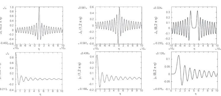
cal and cylindrical Bessel functions is the intensification of contrast from the center towards the periphery, we would expect small, or almost no difference in trends, but eventual increases in sensitivity for cylindri-cal Bessel functions. Figure 1 shows profiles for cylindrical functions, Jn (top), compared
to spherical functions, jn (bottom), for n
values 0, 1 and 8. Figure 2 shows side by side photographs of cylindrical, Jn (right) and
spherical, jn (left) functions for n = 0, 2 and 8.
Figure 3 shows profiles of j4 (µ) for
dif-ferent radial frequencies, i.e., n-order = 4 (constant) with varying radial frequencies, while Figure 4 shows photos of stimuli at n = 0.4 and 8 at radial frequencies of 0.5 and 3.0 cpd (as originally drawn for our experi-ment run at 1.5 m distance).
In the present study, in addition to report-ing data for two different experiments, in detail we compare contrast thresholds to spherical Bessel functions with cylindrical ones for n-order 0 (zero), a comparison not previously made in the literature. We com-pare measurements of contrast thresholds for radial frequency stimuli modulated by jn
of Bessel profiles of j0, j1, j2, j4, j8 and j16 with
those performed for J0.
Method
Subjects
Eight 19- to 42-year-old naive subjects with normal or corrected vision participated in the experiments. Most of the participants were selected among undergraduate students interested in carrying out research on vision at our laboratory. Both authors participated in some measurements and were naive with respect to the specific experiment as well as to the expected results.
Equipment and stimulus material
Circular stimuli measuring 7.25 degrees of visual angle in diameter were generated targets to be much lower than to gratings, no
further work on the subject was done until 1982. In that year, Kelly (9) repeated part of the work of 1975 and went on to use circu-larly symmetric stimuli in a later study (10). In the latter, he also used concentric cosines to evaluate spatial summation.
Few other investigators came close to applying these concepts. Only recently did Amidor (11) and Wilkinson et al. (12) use the term radial frequency to refer to different meanings of modulations, some of them con-cerning modulations across the radius. Main-stream research seems to be more directed towards local filtering of spatial characteris-tics employing Gabor’s or DOG functions as elementary stimuli, generally defined in Car-tesian coordinates to probe local processing (e.g., 13-19).
Dodwell (20) has proposed a Lie trans-formation group model based on Hoffman’s suggestion (21). These researchers see filter-ing in polar coordinates as a by-product of their model. Also, along Dodwell’s line, Gallant, Van Essen and colleagues (22,23) used sine wave and square radial and angu-lar frequency targets to test the sensitivity of V4 cells in macaques.
The studies cited above contain all or most of the literature on the subject.
In our original work published in 1985 and 1990 (1,2), we conceived the visual system in terms of spherically shaped eyes processing visual information and replaced Kelly’s (7) suggestion of cylindrical Bessel function (mathematical notation Jn) with the
choice of spherical ones (mathematical no-tation jn, see Appendix).
Even if we assume simultaneous sepa-rate decompositions by each retina, this sub-stitution of cylindrical by spherical should be made because each eye constitutes spheres upon which spatial information is projected. We could only consider cylindrical Bessel functions for 2-D surfaces or for extremely restricted areas at the center of the eye.
spheri-on a standard 21" TV display (Telefunken with a standard resolution of 250 lines and medium-low contrast resolution) by a 486 PC through a DT2853 frame grabber with RGBsync output. Measurements were made binocularly at a 150-cm distance with a mean luminance equal to 1.8 fL, or 6.2 cd/m2
. This luminance level is necessary in order to run a forced choice procedure since we have to display mean luminance within the linearity of the TV monitor at human threshold levels. Contrast was defined as usually done in the literature on spatial vi-sion, i.e., Lummax - Lummin/Lummax + Lummin.
In the first experiment we used radial frequencies of 0.2, 0.3, 0.5, 0.8, 1, 2, 3, 4, 5, 6 and 9 cycles per degree of visual angle, cpd, modulated by both Jn (r) and jn (r)
profiles of n-order 0 (zero) to characterize each curve. Figure 2 shows examples of Jn (r)
(right) and jn (r) (left) profiles for n-orders 0,
2 and 8 (from top to bottom, respectively). In the second experiment we used the same set of radial frequencies but modulated by jn (r) profiles of n-orders 0, 1, 2, 4, 8 and
16. The same measurements of the jn (r)
profile, n-order 0 (zero) were used for both
Figure 2. Photographs of spheri-cal Bessel functions, jn (left), and cylindrical Bessel functions, Jn (right), for n = 0 (top), n = 2 (cen-ter) and n = 8 (bottom). experiments. Figure 5 shows profiles
origi-nally obtained for n = 0 (top left), 1 (top right), 2 (center left), 4 (center right), 8 (bottom left) and 16 (bottom right) at 1-cpd radial frequency as calibrated under the spe-cific experimental conditions used.
Figure 1. Profiles of cylindrical Bessel functions, Jn (top), and spherical Bessel functions, jn (bottom), for n = 0 (left), n = 1 (center) and n = 8 (right). Profiles of jn (bottom) are defined only for n from 0 (zero) to infinity.
Jn
(0,2
p
h
)
1
jn
(0,2
p
h
)
-0.2 0 1.0 0.8 0.6 0.4 0.2
-0.2 -0.4 0
-0.6 -10
-10 -8 -6 -4 -2 0 2 4 6 8 10 10
h
0.8 0.6 0.4 0.2
-0.4 0 1 2 3 4 5 6 7 8 9 10
h
-0.217 -0.402
1
Jn
(1,2
p
h
)
0.581
jn
(1,2
p
h
)
-0.1 0 0.6
0.4
0.2
0
-0.2
-0.6 -0.4
-10
-10 -8 -6 -4 -2 0 2 4 6 8 10 10
h
0.4
0.3 0.2 0.1
-0.2 0 1 2 3 4 5 6 7 8 9 10
h
-0.168 -0.581
0.436
Jn
(8,2
p
h
)
0.324
jn
(8,2
p
h
)
-0.1 0.3 0.2 0.1 0
-0.2 -0.1
-10
-10 -8 -6 -4 -2 0 2 4 6 8 10 10
h
0.1
0.05
0
-0.05
0 1 2 3 4 5 6 7 8 9 10
h
-0.075 -0.233
1 2 3 4 5 6 7 8 9 10
Figure 3. Profiles of spherical Bessel functions, jn (µ), for n = 4, at varying radial frequencies (µ = 0.3x, 0.5x, left; 1x, 2x, center, and 3x and 4x, right).
jn
(4,2
p
0.3x)
0.202
jn
(4,2
p
0.5x)
-0.1 0 0.25
0.15 0.1 0.2
0 -0.05 0.05
-0.1
0 1 2 3 4 5 6 7 8 9 10 0.25
0.2 0.15 0.1
-0.05
0 1 2 3 4 5 6 7 8 9 10 x
-0.107 -0.107
-0.15
0.05
-0.15
0 10
jn
(4,2
p
1x)
0.202
jn
(4,2
p
2x)
-0.1 0 0.25
0.15 0.1 0.2
0 -0.05 0.05
-0.1
0 1 2 3 4 5 6 7 8 9 10
0.25 0.2 0.15 0.1
-0.05
0 1 2 3 4 5 6 7 8 9 10 x
-0.107 -0.107
-0.15
0.05
-0.15
0 10
jn
(4,2
p
3x)
jn
(4,2
p
4x)
-0.1 0 0.15
0.05
0 0.1
-0.1 -0.15 -0.05
0 0.25
0.2 0.15 0.1
-0.05
0 1 2 3 4 5 6 7 8 9 10 -0.107
-0.107
0.05
-0.15 0.169
Figure 4. Photographs of spherical Bessel functions, jn (µ), for n = 0, n = 4 and n = 8 (top, center, bottom) at µ = 0.5 (left) and 3.0 cpd (right) as originally calibrated for a 150-cm viewing distance.
Figure 5. Stimuli defined by spherical Bessel function profiles originally taken for n = 0 (top left), n = 1 (top right), n = 2 (center left), n = 4 (center right), n = 8 (bottom left) and n = 16 (bottom right) at 1-cpd radial frequency as calibrated under the specific experimental conditions.
-0.202
Procedure
In the first experiment we had eight sub-jects (TPL, ALL, MMM, ERB, SAL, NAS, FMR and MLS) and each of the 11 radial frequencies of jn (r) (n = 0) was measured
three times, on different days, using a forced-choice method (24). For Jn (r) (n = 0)
meas-urements were made under the same condi-tions but with only five subjects (TPL, ALL, MMM, ERB and SAL). The order of meas-urement for conditions and curves was ran-dom for each observer. A whole curve was measured per day. In every experimental session pairs of stimuli were presented cen-tered on the screen at the same site over two different time intervals: one contained one of the radial frequencies and the other was merely a circle at mean luminance. The same radial frequency was presented throughout an entire session. Each stimulus was pre-sented over a period of 2000 ms. The inter-stimulus interval lasted 1000 ms, whereas the intertrial interval lasted 3000 ms follow-ing the answer of the subject. The task of the observer was to correctly select the stimulus containing the radial frequency. The crite-rion was to lower contrast by 0.8% after three correct choices and to increase it by the same amount after each subject’s error. A session was terminated after obtaining 20 estimates, i.e., 10 pairs of peaks and valleys. In the second experiment, j1, j4, j8 and j16
Bessel profiles characterized by the same set of 11 radial frequencies were measured three times each by each of five subjects (TPL, ALL, NAS, FMR and MLS), for a total of 132 experimental sessions per subject (not including those of the first experiment). The remaining procedure and conditions were exactly as described above. The j2 Bessel
profile was measured three times by only three subjects (NAS, FMR and MLS).
Results
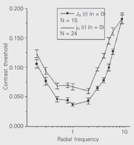
Figure 6 shows contrast thresholds for
radial frequencies modulated by Jn (r) and
jn (r) Bessel profiles of n-order 0 (zero).
Thresholds were lower for cylindrical pro-files for all but one point estimate.
Figure 7 shows the contrast thresholds for radial frequencies modulated by jn (r)
Bessel profiles of n-orders 0 (zero), 1, 2, 4, 8 and 16.
Contrast sensitivity (i.e., the reciprocal of the contrast threshold) is increased with the jnorder for n greater than zero. We can
observe distinct order effects at the low and high frequency ends for increasing n. Stimuli
having j8 and j16 profiles are the most
diffi-cult to detect at the low frequency end, whereas these tend to be the easiest at the high frequency end.
Also, for Bessel profiles j0, j1, j2 and j4,
maximum sensitivity tends to occur at the 0.8-to 1-cpd interval, while for the j8 and j16
pro-files this sensitivity appears to shift gradually to the 0.8- to 3-cpd interval. For the j16 profile,
maximum sensitivity for all observers was in the 2- to 3-cpd radial frequency interval. We believe this is due to increased iso-luminance at the center of the stimuli which occurs with increasing n-order. That is to say that the task of detection of these stimuli is shifting towards the periphery. We did not study enough n-orders to observe at what radial frequency this shifting stabilizes.
Contrast threshold
0.200
0.150
0.100
0.050
0.000
1 10
Radial frequency Jn (r) (n = 0) N = 15
N = 24
jn (r) (n = 0)
Our statistical treatment was to estimate the standard error of the mean for each distri-bution of 180-300 values measured (within and across subjects) per point and correct for sample size using the t-Student statistic to
obtain the 99% confidence level.
In previous studies we have demonstrated that this corrected estimate is more rigorous than testing means by comparison for two correlated samples or by ANOVA treatment. Using the confidence level method, when two error bars show a 50% overlap, if we calculate the t-statistic obtained by testing
difference between two means for correlated samples, we find a significance of at least P = 0.05, and sometimes smaller. In our treatment, most of the error bars that do not overlap would show a significance of P<0.000 if a t-test for comparison of means
for correlated samples were performed. The use of ANOVAS (very traditional in psy-chology) in this case tends to show signifi-cant effects in all factors and interactions and does not add much information.
Discussion
As expected, sensitivity was higher for cylindrical Bessel profiles. Since the differ-ence in peak at zero and modulation of pe-riphery is higher for spherical profiles (see Figure 1) we did expect higher sensitivities for cylindrical profiles because, as one can see in Figures 1 and 2, contrast at the periph-ery is perceived as higher than that for spheri-cal profiles. However, to study the expan-sion effects of increasing the n-order, we used spherical profiles because of the spheri-cal shape of the eyes (and retina).
Figure 8 also shows the comparisons be-tween sensitivity to sine wave gratings, cy-lindrical Bessel J0, angular frequencies and
coupled radial/angular frequencies of n-order equal to 4. Note that Figure 8 shows contrast thresholds rather than sensitivity.
We also obtained results comparing row-band spatial frequency filters to nar-row-band radial frequency filters modulated by j0, j1, j4, j8 and j16 Bessel profiles and
Contrast threshold
0.250
0.200
0.150
0.100
0.050
0.000
jn (r) (n = 0) (N = 24)
Contrast threshold
0.200
0.150
0.100
0.050
0.000
jn (r) (n = 1) (N = 15)
Contrast threshold
0.200
0.150
0.100
0.050
0.000
jn (r) (n = 2) (N = 9)
Contrast threshold
0.200
0.150
0.100
0.050
0.000
jn (r) (n = 4)
(N = 15)
Contrast threshold
0.250
0.200
0.150
0.100
0.050
0.000
jn (r) (n = 8)
(N = 15)
Contrast threshold
0.200
0.150
0.100
0.050
jn (r) (n = 16)
(N = 15)
1 10
Radial frequency
1 10
Radial frequency
0.1 1 10
Radial frequency
1 10
Radial frequency
1 10
Radial frequency
1 10
Radial frequency
centered at radial frequencies of 1 and 4 cpd (Simas MLB, Frutuoso JT and Santos NA, unpublished results). These results are con-sistent with the possible existence of nar-row-band radial frequencies that seem to operate linearly at higher contrast levels than spatial frequency filters, as shown by a supra-threshold summation paradigm.
Although the results reported here are only for the radial part, because we used n>0, they should be considered together with the orthogonal part, i.e., as angular frequen-cies because when n>0 the angular compo-nent is also present.
Filtering of radial and angular frequencies by the visual system
Our studies of 1985 (1), 1990 (2) and 1992 (3) on angular frequency detection and filtering by the human visual system should be considered in relation to the data reported here. Selective neighboring inhibition around the testing frequency was consistently ob-served for angular frequency filters of 2, 4, 9, 13, 16, 24 and 47 cycles (3). The previous results were obtained with the use of phases different from those we use today. The study was carried out only with 24 cycles (1,2).
Those results, together with the findings of Gallant and colleagues (22,23) about groups of cells selective for angular and radial frequencies strongly encouraged us to proceed with our psychophysical studies in that direction. To our knowledge, except for Kelly’s early study (7), no investigations were carried out with targets modulated by Bessel functions, or perhaps circular cosine functions. These are not equivalent and Kelly and Magnuski (8) measured them both.
To better evaluate filtering of radial and angular spatial frequencies by the human vi-sual system we should point out that when n = 0 in Equation 4, only the radial part exists, precisely the Jo (we preferred j0) part pointed
out by Kelly (7). This part is well suited to describe retinal acuity and light intensity
cen-tered in fovea and near fovea regions. The angular part would be zero, i.e., mean lumi-nance. When this happens, higher luminance levels are required as compared to both sensi-tivity to gratings and to angular frequencies.
The opposite situation, i.e., only the an-gular component, would occur when the stimulus has radial frequencies in the lowest range of the radial spectrum so that a large portion of a cycle is present. In this case, light intensity would not be concentrated at the fovea and would spread evenly across large portions of the visual field except for the modulation of the angular part present. This could occur for any n>0, but may occur more commonly for n>8. The angular part would be always present for n>0 and the
Figure 8. Comparisons between contrast thresholds for sine wave gratings (i.e., reciprocal of contrast sensitivity function, 1/CSF, dark square), cylindrical Bessel J0 (i.e., 1/radial CSF, rCSF, triangle), angular frequencies (i.e., 1/angular CSF, 1/aCSF, circle) and coupled radial/ angular frequencies of n-order equal to 4 (i.e., JF04, light square).
Contrast threshold
0.400
0.300
0.200
0.100
0.000
1 100
Spatial frequency (cpd) and angular frequency (integer) 1/CSF (n = 3)
1/aCSF (n = 15)
rCSF (J0) (n = 4)
JF04 (n = 5)
exact number and values of n would depend
on the particular visual system in question. For the human visual system, the angular modulation transfer function ranges from 1 to 100 cycles (we made n = integer, to fit exactly in 360 degrees) (1,2,4).
Since we were also interested in learning how this filtering process could be involved in face detection and/or recognition, in a related study on narrow-band angular frequency fil-ters we presented the face of the night monkey aotus as an example showing that the angular part appears to be somewhat dominant over the radial one, particularly at 1, 2, 3 and 4 cycles (25). We also find it interesting that the aotus has nocturnal habits because if we con-sider very low angular frequencies such as these, very large portions of the retina would be involved in visually processing information and thus would require (work best under) lower luminance levels.
If we assume that the visual system of an organism must have the necessary character-istics to recognize its own species, as shown in the literature (26,27), we could try to predict maximum sensitivity to radial fre-quencies for certain species. In this case, we could take into consideration base focal dis-tance together with the typical size of their faces in their habitat. It would be just a matter of calculating for a given distance which first minimum of radial frequency would coincide with their black/white re-gions around the eyes and head. If the angu-lar component is present, this would show on the face of a given species, particularly for those species using few low angular fre-quency filters. Note that the tuning for spa-tial frequencies is not necessarily equivalent to that for radial frequencies. For example, the human visual system is tuned to 3-4 cpd for spatial frequencies and 0.8-2.0 cpd for radial frequencies of n = 0 profiles.
Since it is very unlikely that all organ-isms having circular pupils will have a com-plete set of all radial and angular frequency components, a few animals possessing less
developed visual systems could show their most basic angular/radial filters on their own patterned faces. The aotus would be a good example for low n, i.e., 2, 3 and 4.
If we bear in mind that, as we proceed to select phases for the angular frequency stimuli, we find that for an even n there could
be symmetry among quadrants, whereas for an odd n there could be symmetry between
hemispheres, this would have strong impli-cations in visual projections from one area to another and among different species. Ani-mals having homogeneously colored faces, less protruding noses, etc., would need more complete sets to process spatial information. In this case, they could develop coupled radial and angular frequencies presenting n = even and n = odd-even series. An ex-ample of n = even series is 2, 4, 8, 16 cycles, etc. An n = odd-even series would be 1, 2, 3, 4, 6, 8, 12, 16, etc. If we consider that n = even harmonic series may suffer biologi-cal “up-grades” more easily, n = even series would be more frequent in lower species. Since n = odd series may require hemi-spheric symmetry, angular frequencies of 1, 2, 3, 5, 7 cycles, etc., would be originators of sub-series.
Thus, in the present study we are just starting to explore how the human visual sys-tem responds as we manipulate the elementary frequency stimulus sets of the radial compo-nent. We observed that as n is increased (n>0),
maximum sensitivity tends to be displaced to higher frequencies even though the absolute value of the contrast threshold may remain in the same range as for low n. Since we used
n>0, the angular component is also relevant. We already have some initial results from studies coupling angular and radial compo-nents which show that adding the angular part to jn increases overall sensitivity.
References
1. Simas ML de B (1985). Linearity and do-main invariance in the visual system. Doc-toral thesis, Queen’s University at King-ston, Ontario, Canada. University Micro-films International. Ann Arbor, MI, USA. “Publication No. 86-17940”.
2. Simas ML de B & Dodwell PC (1990). Angular frequency filtering: a basis for pat-tern decomposition. Spatial Vision, 5: 59-74.
3. Simas ML de B, Frutuoso JT & Vieira FM (1992). Inhibitory side bands in multiple angular frequency filters in the human vi-sual system. Brazilian Journal of Medical and Biological Research, 25: 919-923. 4. Simas ML de B, Santos NA dos & Thiers
FA (1997). Contrast sensitivity to angular frequency stimuli is higher than that for sinewave gratings in respective middle range. Brazilian Journal of Medical and Biological Research, 30: 633-636. 5. Simas ML de B & Santos NA (1997).
Hu-man visual contrast detection of radial fre-quency stimuli defined by Bessel profiles j0, j1, j2, j4, j8 and j16 and its relation to angular frequency. Proceedings of the II Workshop on Cybernetic Vision, IEEE Computer Science, Los Alamitos, CA, USA, 219-224.
6. Simas ML de B & Santos NA (1998). Hu-man frequency response functions of har-monic 2, 4, 8 and 16 cycles angular fre-quency filters. Proceedings of the Inter-national Symposium on Computer Graph-ics, Image Processing and Vision, IEEE Computer Science, Los Alamitos, CA, USA, 312-319.
7. Kelly DH (1960). Stimulus pattern for vi-sual research. Journal of the Optical Soci-ety of America, 50: 1115-1116.
8. Kelly DH & Magnuski HS (1975). Pattern detection and the two-dimensional Fou-rier transform: circular targets. Vision Re-search, 15: 911-915.
9. Kelly DH (1982). Motion and vision. IV. Isotropic and anisotropic spatial re-sponses. Journal of the Optical Society of America, 72: 432-439.
10. Kelly DH (1984). Retinal inhomogeneity. I. Spatiotemporal contrast sensitivity. Jour-nal of the Optical Society of America A, 1: 107-113.
11. Amidor I (1997). Fourier spectrum of radi-ally periodic images. Journal of the Opti-cal Society of America A, 14: 816-826. 12. Wilkinson F, Wilson HR & Habak C (1998).
Detection and recognition of radial fre-quency patterns. Vision Research, 38: 3555-3568.
13. Pollen DA, Nagler M, Daugman JG, Kroaner R & Koenderink JJ (1984). Use of Gabor elementary functions to probe re-ceptive field substructure of posterior inferotemporal neurons in the owl mon-key. Vision Research, 24: 233-242. 14. Graham N, Sutter A & Venkatesan C
(1993). Spatial-frequency- and orientation-selectivity of simple and complex chan-nels in region segregation. Vision Re-search, 33: 1893-1911.
15. Hess RF & Hayes A (1994). The coding of spatial position by human visual system: Effects of spatial scale and retinal eccen-tricity. Vision Research, 34: 625-643. 16. Hess RF & Wilcox LM (1994). Linear and
non-linear filtering in stereopsis. Vision Research, 34: 2431-2438.
17. Hess RF & Field DJ (1995). Contour inte-gration across depth. Vision Research, 35: 1699-1711.
18. Peli E, Arend L & Labianca AT (1996). Contrast perceptions across changes in luminance and spatial frequency. Journal of the Optical Society of America A, 13: 1953-1959.
19. Graham N & Sutter A (1998). Spatial sum-mation in simple (Fourier) and complex (non-Fourier) texture channels. Vision
Re-search, 38: 231-257.
20. Dodwell PC (1983). The Lie group trans-formation model of visual perception. Per-ception and Psychophysics, 34: 1-16. 21. Hoffman WC (1966). The Lie algebra of
visual perception. Journal of Mathemati-cal Psychology, 3: 65-98. Errata, ibid., 4 (1967), 348-440.
22. Gallant JL, Braun J & Van Essen DC (1993). Selectivity for polar, hyperbolic, and Cartesian gratings in macaque visual cortex. Science, 259: 100-103.
23. Gallant JL, Connor CE, Rakshit S, Lewis JW & Van Essen DC (1996). Neural re-sponses to polar, hyperbolic, and Carte-sian gratings in area V4 of the macaque monkey. Journal of Neurophysiology, 76: 2718-2739.
24. Wetherill GB & Levitt H (1965). Sequen-tial estimation of points on a psychomet-ric function. British Journal of Mathemati-cal and StatistiMathemati-cal Psychology, 18: 1-10. 25. Simas MLB & Santos NA (2002).
Narrow-band 1, 2, 3, 4, 8, 16 and 24 cycles/360º
angular frequency filters. Brazilian Journal of Medical an Biological Research, 35: 243-253.
26. Bruce CJ, Desimone R & Gross CG (1981). Visual properties of neurons in a polysen-sory area in superior temporal sulcus of the macaque. Journal of Neurophysiology, 46: 369-384.
27. Desimone R (1991). Face-selective cells in the temporal cortex of monkeys. Jour-nal of Cognitive Neuroscience, 3: 1-8. 28. Mortensen U & Meinhardt G (2001).
Appendix
Angular frequencies as elementary stimuli
Despite the fact that if we adopt a polar coordinate system it is necessary to divide elementary stimuli into two components, i.e., radial and angular, in his original proposal, Kelly (7) defined only the radial part as cylindrical Bessel functions of zero order and left out the angular part.
In 1985, Simas (1), using an equation from Sneddon (29) defining a Hankel series, introduced the idea of angular frequency stimuli as the orthogonal component of radial frequencies, i.e. defined by Kelly as Jn targets.
From Sneddon’s equation describing a series defined in polar coordinates:
¥
exp(ixsinq) = S Jn(x)einq (Equation 1)
n = -¥
where Jn(x) is the radial part and einq the angular one,we substituted x for 2prr:
¥
exp(i2prrsinq) = S Jn(2prr)einq (Equation 2)
n = -¥
and made:
einq
= cos(nq) + i sin(nq). (Equation 3)
Thus,
¥
exp(i2prrsinq) = S Jn(2prr) {cos(nq) + i sin(nq)} (Equation 4)
n = -¥