On the use of Schwarz–Christoffel conformal mappings to the grid generation for global ocean models

(1)

GMDD

8, 1337–1373, 2015

Schwarz–Christoffel mapping and grid

generation

S. Xu et al.

Title Page

Abstract Introduction

Conclusions References

Tables Figures

◭ ◮

Back Close

Full Screen / Esc

Printer-friendly Version

Interactive Discussion

Discussion

P

a

per

|

Discussion

P

a

per

|

Discussion

P

a

per

|

Discussion

P

a

per

|

Geosci. Model Dev. Discuss., 8, 1337–1373, 2015 www.geosci-model-dev-discuss.net/8/1337/2015/ doi:10.5194/gmdd-8-1337-2015

This discussion paper is/has been under review for the journal Geoscientific Model Development (GMD). Please refer to the corresponding final paper in GMD if available.

On the use of Schwarz–Christo

_ff

el

conformal mappings to the grid

generation for global ocean models

S. Xu1, B. Wang1,2, and J. Liu3

1

Ministry of Education Key Laboratory for Earth System Modeling, Center for Earth System Science (CESS), Tsinghua University, Beijing, China

2

State Key Laboratory of Numerical Modeling for Atmospheric Sciences and Geophysical Fluid Dynamics (LASG), Institute of Atmospheric Physics, Chinese Academy of Sciences, Beijing, China

3

Department of Atmospheric and Environmental Sciences, University at Albany, State University of New York, Albany, NY 12222, USA

Received: 3 December 2014 – Accepted: 28 January 2015 – Published: 13 February 2015

Correspondence to: S. Xu ([email protected])

(2)

GMDD

8, 1337–1373, 2015

generation

S. Xu et al.

Title Page

Tables Figures

◭ ◮

Back Close

Full Screen / Esc

Discussion

P

a

per

|

Discussion

P

a

per

|

Discussion

P

a

per

|

Discussion

P

a

per

Abstract

In this article we propose two conformal mapping based grid generation algorithms for global ocean general circulation models (OGCMs). Contrary to conventional, analyti-cal forms based dipolar or tripolar grids, the new algorithms are based on Schwarz– Christoffel (SC) conformal mapping with prescribed boundary information. While

deal-5

ing with the basic grid design problem of pole relocation, these new algorithms also address more advanced issues such as smoothed scaling factor, or the new require-ments on OGCM grids arisen from the recent trend of high-resolution and multi-scale modeling. The proposed grid generation algorithm could potentially achieve the align-ment of grid lines to coastlines, enhanced spatial resolution in coastal regions, and

10

easier computational load balance. Since the generated grids are still orthogonal curvi-linear, they can be readily utilized in existing Bryan–Cox–Semtner type ocean models. The proposed methodology can also be applied to the grid generation task for regional ocean modeling where complex land–ocean distribution is present.

1 Introduction 15

The generation of the horizontal model grid preludes the simulation with general ocean circulation models (OGCMs) and sea ice models. Among state of the art OGCMs, in-cluding those participating in Coupled Model Intercomparison Project, the fifth phase (CMIP5 CMI, 2014) and global oceanic forecast (e.g., Metzger et al., 2014; Storkey et al., 2010), the majority of them use general orthogonal grids generated from

ana-20

lytical forms. These dipolar or tripolar grids may be generated from a simple Mobius Transformation, or orthogonal curves, as in Murray (1996); Murray and Reason (2001). The major purpose is to avoid the explicit North Pole which resides in the oceanic area in the latitude-longitude grid. The design choice deals with both efficiency and precision issues: (1) to alleviate the severe time step constraints and low efficiency caused by

25

(3)

GMDD

8, 1337–1373, 2015

generation

S. Xu et al.

Title Page

Tables Figures

◭ ◮

Back Close

Full Screen / Esc

Discussion

P

a

per

|

Discussion

P

a

per

|

Discussion

P

a

per

|

Discussion

P

a

per

|

the error caused by grid size anisotropy near the poles. Hence, these grid generation methods only deal with the question of which land position(s) the pole is relocated to. Very limited consideration in terms of computation and simulation precision is taken to further exploit the land–sea distribution.

Contrary to global models, regional ocean models usually utilize curvilinear

coor-5

dinates that follow coastlines, instead of the grid based on analytical forms. This is an established practice, covering the range of the small-scale phenomena study such as river plumes (Gan et al., 2009), to large or basin scale modeling such as Xu and Oey (2011). The motivations for curvilinear coordinates in regional models are from both computational efficiency and precision aspects: (1) the alignment of grid lines with

10

coastlines and/or isobaths is of potential benefit to better simulation, such as river dis-charge and more realistic topographic forcing on the oceanic flow; and (2) the removal of land in the computational domain results in lower computational overhead since lands no longer occupy the grid system. Example grid generation tools such as Sea-Grid (Sea, 2014) use conformal mapping to generate an orthogonal, logically cartesian

15

grid. In SeaGrid, heuristics is required for the actual construction of the mapping, by pre-defined vertices of the region to be modeled.

One recent trend in geophysical fluid modeling is high resolution simulation: up to 0.1◦ or higher have been successfully applied to global models and used in both cli-mate research as in Dennis et al. (2012) and forecast operations such as Metzger et al.

20

(2014). These high resolution (higher than 0.1◦) already overlaps with the resolution range in conventional regional ocean models. Although small scale phenomena could be explicitly resolved, such as narrow yet important water channels and mesoscale ed-dies, the model is usually very computationally demanding. Trade-offs usually have to be taken between simulation precision (i.e. spatial resolution) and computational cost.

25

(4)

GMDD

8, 1337–1373, 2015

generation

S. Xu et al.

Title Page

Tables Figures

◭ ◮

Back Close

Full Screen / Esc

Discussion

P

a

per

|

Discussion

P

a

per

|

Discussion

P

a

per

|

Discussion

P

a

per

ocean usually feature different spatial scales. For example, the first baroclinic defor-mation radius of the ocean (Chelton et al., 1998) changes according to latitude, ocean stratification and depth, which serves as a good reference of how much resolution is actually needed for eddy resolution. By using multi-scale modeling with spatial refine-ment for when or where necessary (e.g., Mandli and Dawson, 2014; Ringler et al.,

5

2013), the prohibitively high cost of high-resolution models may be partially alleviated, and potentially better simulation could also be achieved.

In this paper, we consider these issues, including the recent trend of high-resolution modeling, from the perspective of grid design. We believe that a well designed model grid could potentially contribute to better simulation and higher computational efficiency.

10

To begin, we first summarize the desired properties of the grid for global OGCMs as follows. They are loosely sorted according to relative importance, starting from more important or classic ones to less important or more modern ones.

1. Grid orthogonality.

2. Relocation of grid poles to land. The further these artificial poles are from the

15

ocean, the better.

3. The scaling factor evolves continuously, i.e., there is no jump of local grid sizes.

4. The grid is longitudinal and latitudinal along the equatorial regions, which also facilitates spatial refinements.

5. Grid size anisotropy should be low.

20

6. Major oceanic area is still covered with regular latitude-longitude grid.

7. The grid is indexable as a cartesian grid.

8. Reduction of unused grid points (i.e., grid points on lands) as many as possible.

(5)

GMDD

8, 1337–1373, 2015

generation

S. Xu et al.

Title Page

Tables Figures

◭ ◮

Back Close

Full Screen / Esc

Discussion

P

a

per

|

Discussion

P

a

per

|

Discussion

P

a

per

|

Discussion

P

a

per

|

This list is arguably more comprehensive than that in Roberts et al. (2006). The subset of the first four items coincides with the whole list in Roberts et al. (2006). For the sake of higher precision near the poles, the fifth item emphasizes on the scale difference in two directions for effective resolution near the poles. Item 6 through 8 con-cerns computational aspects. If most part of the general orthogonal grid is still

latitude-5

longitude grid, the memory usage could be saved by storing only two vectors of the latitude and longitude, instead of the position information of all the cell centers and vertices. Since OGCMs usually utilize parallel computation with 2-D domain decompo-sition, a logically cartesian grid is both intuitive and easy in terms of implementation, for both domain decomposition and communication management. We denote the

log-10

ical indexation of the model grid as the grid index space. For item 8, since grid cells dedicated to land do not participate in the computation and communication in OGCM simulation, reducing their total number or proportion in the grid index space could im-prove e_fficiency and potentially exempts the need for load balancing. Item 9 is related to the aforementioned new trends of high-resolution and multi-scale simulation. It is

15

desirable that the grid could achieve higher spatial resolution in place of need (such as coastal and comparatively shallow oceanic regions and polar regions) and alignment of coastlines to grid lines as in regional ocean models.

The most widely used grid used in current global OGCMs include dipolar grids with the relocated North Pole, and tripolar grids with the North Pole split and relocated onto

20

lands (see Murray, 1996 for a comprehensive set of grids). The design of these grids mainly concerns the first 7 items in the list. For example, the alleviation of the scale changes across patches are achieved in Roberts et al. (2006). However, most existing model grids do not address the last two items on the list. Finite-Elements methods based OGCMs or those supporting irregular meshes (e.g., Chen et al., 2006; Wang

25

(6)

GMDD

8, 1337–1373, 2015

generation

S. Xu et al.

Title Page

Tables Figures

◭ ◮

Back Close

Full Screen / Esc

Discussion

P

a

per

|

Discussion

P

a

per

|

Discussion

P

a

per

|

Discussion

P

a

per

1.1 Schwarz–Christoffel conformal mapping

Conformal mapping (Nehari, 1975) are angle-preserving transformation on the com-plex plane, i.e., two-dimensional domain. Although it usually falls into the domain of complex analysis in mathematics, due to its close relationship with potential theory and Laplacian Equations, it could be applied to transform complicated boundaries to

5

simpler configurations that are is easy to analyze and process. Its wide application in engineering is mainly based on the fact that the solutions to Laplacian Equations re-main invariant under conformal mappings. Examples include electrostatics, fluid flow, steady-state heat conduction, etc. (Schinzinger and Laura, 1991). Existing grid gener-ation methods already utilizes conformal mappings to the genergener-ation of grids.

Gener-10

ation of conventional dipolar and tripolar grids exploits: (1) the conformal behavior of stereographic projections, (2) the equivalence of the projection of the sphere (or earth) and the complex plane, and (3) conformal mapping on the complex plane to achieve North Pole relocation, etc.

For a single-connected region on the complex plane, the famous Riemann Mapping

15

Theorem guarantees the existence of the conformal mapping between an enclosed re-gion to a unit disk, with the conformal center (invariant point with the mapping) mapped to the origin of the disk. The polar coordinates can be constructed on the unit disk, and mapped to the predefined enclosed polygon region to form the orthogonal grid. With the conformal mapping, an orthogonal grid system is constructed for this region. The

20

most simple example is the Mobius Transformation, which could be used to relocate the conformal center, given that the boundary is a disk. This characteristics is exploited in earlier OGCM grid generation algorithms to achieve the relocation of the North Pole, as summarized in Murray (1996).

For a region with a boundary that could not be trivially defined as a circle, more

25

(7)

GMDD

8, 1337–1373, 2015

generation

S. Xu et al.

Title Page

Tables Figures

◭ ◮

Back Close

Full Screen / Esc

Discussion

P

a

per

|

Discussion

P

a

per

|

Discussion

P

a

per

|

Discussion

P

a

per

|

and internal angles at corresponding vertices{φ_i|1≤i ≤n}, the SC mapping f from the unit disk to this enclosed polygon could be defined as:

f(z)=A₊C z

Z n Y

i=1

1− ζ z_i

_φi π

dζ (1)

Where A and C are scalar constants, and z_i’s are pre-vertices to be mapped to corresponding v_i’s. These values are actually parameters to constrain the mapping

5

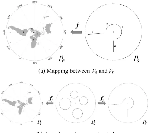
to be between a unit circle to the predefined polygon. They can be solved through a nonlinear solution process and computation of Schwarz–Christoffel integrals. Please refer to Driscoll and Trefethen (2002) for corresponding algorithms and SCToolBox (SCT, 2014) for a MATLAB implementation. SCToolBox is also used to generate the mapping and corresponding polar grid in Fig. 1.

10

For a multiple-connected region with connectivity ofn(2< n <∞), i.e., a region with

n−1 closed, non-intersecting polygons, there exists canonical forms that this region could be mapped to (Chapter 7 of Nehari, 1975). Figure 2 shows a sample polygon based region with connectivity of 5, and several canonical forms of the whole com-plex plane that it could be mapped to. The canonical forms with slits are shown in

15

the last three subfigures. The actual construction theories for this type of mappings have witnessed breakthrough in the recent decade since Delillo et al. (2004). For the construction algorithms based on reflection principle and Laurent Series expansion, please refer to DeLillo and Kropf (2011); DeLillo et al. (2013) for details. In this article, we mainly utilize the implementation for Laurent Series expansion for external MCSC

20

maps in DeLillo et al. (2013) and the open-source software of MCSC (MCS, 2014) for the actual mapping construction process. We also follow the naming convention of multiply connected Schwarz–Christoffel mapping (MCSC), and use SCSC for abbrevi-ations for Schwarz–Christoffel mapping for single-connected regions.

In this paper, we propose two new methods based on SC mappings for the grid

25

(8)

GMDD

8, 1337–1373, 2015

generation

S. Xu et al.

Title Page

Tables Figures

◭ ◮

Back Close

Full Screen / Esc

Discussion

P

a

per

|

Discussion

P

a

per

|

Discussion

P

a

per

|

Discussion

P

a

per

new algorithms are targeted to meet a broader range of the aforementioned proper-ties of global OGCM grid. The SC mapping is utilized to accommodate user-specified boundaries during the grid generation process. In the first method, we tackle the con-ventional design problem (item 1 through 7) for dipolar grids with patches. Contrary to a longitudinal boundary between patches (as in Murray, 1996; Roberts et al., 2006),

5

we use a non-longitudinal, irregular boundary for the North Polar region. The sam-ple grid achieves a higher latitude-longitude proportion of the grid than conventional dipolar grids, and ensures smooth scaling factor changes across patch boundaries. Specifically, an SCSC mapping is used for the grid construction in the North Polar re-gion. The second grid generation method is based on MCSC, and it aims to tackle the

10

emerging trends of high-resolution and multi-scale modeling from the perspective of grid design (item 8 and 9). By using the inner boundaries of major continental masses, an MCSC mapping is constructed between the earth under stereographic projection and a complex plane on which these boundaries are mapped to slits with no area. The result grid effectively removes major continental area that are within the closed

bound-15

aries, and the grid cells previously dedicated to these continental regions are actually redistributed to oceanic regions, with regions closer to these boundaries (i.e., coastal regions) more densely packed with grid cells, hence better spatial resolution in corre-sponding regions. Besides, smooth grid scale transition to coarser spatial resolution is also guaranteed, since the grid is generated from a single conformal mapping.

20

The following part of the article is organized as follows. Section 2 introduces the first grid generation method with pole relocation and SCSC, and Sect. 3 covers the design of the second method based on MCSC. We also provide a sample grid and basic evaluations for each method. Then in Sect. 4, extensions to these methods, and the relationships with existing methods are discussed. Finally, Sect. 5 concludes the

25

(9)

GMDD

8, 1337–1373, 2015

generation

S. Xu et al.

Title Page

Tables Figures

◭ ◮

Back Close

Full Screen / Esc

Discussion

P

a

per

|

Discussion

P

a

per

|

Discussion

P

a

per

|

Discussion

P

a

per

|

2 Pole relocation with SCSC mappings

In this section we apply the Schwarz–Christoffel mapping for single-connected region to the problem of North Pole relocation for dipolar grids for global OGCMs. In exist-ing patchexist-ing schemes with dipolar grids (Murray, 1996; Roberts et al., 2006), a polar patch is defined to be the area higher than a certain turning latitude (e.g., 30◦N) and

5

the relocation of the North Pole is carried out within this patch, by using an analyti-cal form, such as Mobius Transformation. Contrary to conventional methods, we de-sign a patching strategy with: (1) a North-Polar cap patch with a irregular boundary (instead of a uniform turning latitude), (2) several lower latitude patches with regular latitude-longitude cells on the oceans, and (3) smoothed scale changes across patch

10

boundaries. The patching scheme is shown in Fig. 3. In all 5 patches are created for the whole globe.

The North-Polar cap patch (NP) includes a relocated pole on Greenland, and a smooth, closed, but irregular longitudinal boundary with 4 segments. Two segments of the boundary are longitudinal lines across the Atlantic and Pacific Ocean,

respec-15

tively. They extend into landmass on both ends. The other two segments link up the whole boundary to form a closed and smooth boundary. Due to the irregular boundary of NP, a Schwarz–Christoffel (SC) mapping for singly connection region is constructed. rather than an analytical mapping such as Mobius Transformations. The SC mapping is constructed to: (1) map NP under stereographic projection to a unit disk, (2) map the

20

prescribed position on Greenland to the origin of the unit disk.

Patches southern to NP are constructed as: (1) the southern patch (SP), to cover southern mid-latitudes and high latitudes; (2) equatorial band patch (EBP), to cover areas near the equator with spatial refinement in meridional direction; (3) north-pacific patch (NPP), covering the area that is between EBP and NP on the Pacific Ocean and

25

(10)

GMDD

8, 1337–1373, 2015

generation

S. Xu et al.

Title Page

Tables Figures

◭ ◮

Back Close

Full Screen / Esc

Discussion

P

a

per

|

Discussion

P

a

per

|

Discussion

P

a

per

|

Discussion

P

a

per

Furthermore, we construct the oceanic part of NPP and NAP to be fully latitudinal-longitudinal, hence, orthogonal. The orthogonality of other cells in NPP and NAP, which are all on land, are not mandatory hence not kept. Since these cells do not participate in simulation, it is guaranteed that the non-orthogonality of these cells does not affect simulation results.

5

The scaling factor along NP boundary is not uniform, as is the source of a common shortcoming of patching strategies as in Murray (1996). Because the basins of Atlantic Ocean and Pacific Ocean are not directly linked within 40 and 70◦N, different latitudinal grid steps in these two basins could be used to mitigate the different scale changes across boundaries between NP and NPP, and between NP and NAP.

10

The general algorithm is listed as follows:

1. Generation of NP using predefined boundaries, by a SC mapping from a unit-disk to the stereographic projection of NP. An orthogonal grid is generated for the unit disk in polar coordinates and mapped back by the SC mapping and backward stereographic projection. The scaling factor along the NP boundaries on Pacific

15

Ocean and Atlantic Ocean are computed.

2. Generate the Pacific and North Atlantic basin patches, i.e., NAP and NPP. Linkage between: (1) NAP and NPP on eastern and western boundaries, (2) NAP (or NPP) and NP are also constructed, to keep the continuity of cell positions.

3. Generate equatorial and southern grid, i.e., EBP and SP.

20

4. Combine the patches into a global grid.

5. Generate land and depth masks.

In this grid generation process, several aforementioned grid design issues are addressed, including: (1) the enlargement of the portion of the regular latitudinal-longitudinal part; (2) the mitigation of scale changes across patch boundaries; (3)

(11)

GMDD

8, 1337–1373, 2015

generation

S. Xu et al.

Title Page

Tables Figures

◭ ◮

Back Close

Full Screen / Esc

Discussion

P

a

per

|

Discussion

P

a

per

|

Discussion

P

a

per

|

Discussion

P

a

per

|

reduced grid anisotropy in polar regions, etc. A MATLAB version of the grid genera-tion code is available as open source software based on SCToolBox (SCT, 2014) and related software. Parameters for the grid generation are fully customizable, including: meridional and zonal resolution, equatorial refinement, anisotropy control threshold, etc. A sample grid with approximately 1◦ resolution is shown in Fig. 4, with the North

5

Polar region shown in detail. One in every five lines are shown in both directions. The regular latitudinal-longitudinal part on the Pacific and Atlantic Ocean are clearly shown. The patch boundary between NPP and NAP are shown as non-smooth lines, since the orthogonality in these continental regions is not maintained as mentioned.

2.1 SC mapping of NP 10

The choice for the boundary of NP is the trade-offamong several factors: the reduction of the length of the boundary on the Pacific and Atlantic Ocean, the smoothness of the scaling factor in both meridional and zonal directions, etc. In the sample grid, we choose: (1) on the Pacific side, the longitudinal segment crossing Bering Strait, i.e., at about 66◦N, from 170◦E to 160◦W; (2) on the Atlantic side, the longitudinal segment

15

at about 48◦N, from 70◦W to 0◦E; (3) the smooth linkage between the two segments be constructed on both North American and Eurasian continent. The smoothness is ensured by constructing a cosine function shaped curve in the latitude-longitude space. Suppose we need to link a point at (lat1, lon1) and another point at (lat2, lon2), with smooth linkage to longitudinal lines on both ends. The latitude on a specific point on

20

the link at certain longitude could be written as a function of the longitude:

latitude=lat1+(lat2−lat1)

1−coslongitude−lon1 lon₂−lon₁ ×π

2 (2)

The scheme is also shown in Fig. 6a. Approaching both ends of the link, i.e., (lat1, lon1) and (lat2, lon2), the link is gradually parallel and linked to the specific lon-gitudinal lines. Hence the overall smoothness is kept.

(12)

GMDD

8, 1337–1373, 2015

generation

S. Xu et al.

Title Page

Tables Figures

◭ ◮

Back Close

Full Screen / Esc

Discussion

P

a

per

|

Discussion

P

a

per

|

Discussion

P

a

per

|

Discussion

P

a

per

For the construction of SC mapping, we use a discretized boundary with a certain resolution (e.g., 1◦ in zonal direction), to match the requirement of a polygon boundary for SC mapping. The polygon with latitude and longitude information is mapped to the complex plane under stereographic projection. Then the SCToolBox is used for the construction of the mapping. NP boundary is shown in Fig. 3a in blue color. The grid

5

lines in NP, due to their orthogonality before the SC mapping, are orthogonal after the mapping. This applies both internally and to the boundary. The pole is relocated to Greenland.

2.2 Control of grid anisotropy

For global orthogonal grids, grid cells in the polar regions tend to feature extreme cell

10

size anisotropy, which might affect the effective resolution in these regions. On the contrary, equatorial regions are often modeled with higher meridional resolution for purposes such as to simulate ENSO more precisely Griffies et al. (2000), hence certain grid anisotropy are also present for lower latitudes in models such as POP in CCSM4. In the proposed grid in this section, the anisotropy in polar regions is controlled by

15

a bespoken threshold. This threshold is set to be the same value as that used for the equatorial meridional grid refinement, hence the maximum grid size anisotropy of the whole grid is kept below this value. This design choice is hard-wired to the code but changeable according to user choices. For SP, due to that it is purely latitudinal and longitudinal, the latitudes and longitudes of the grid points could be computed

20

as one dimensional arrays. We start from the lowest latitude (southern boundary of EBP) and integrate to higher latitudes by latitudinal step sizes, and decrease latitudinal steps gradually to make sure the maximum anisotropy does not increase beyond the predefined threshold. For NP, a similar strategy to reduce the latitudinal steps is used, except that due to the uneven cell sizes for a given zonal circle, the anisotropy of

25

(13)

GMDD

8, 1337–1373, 2015

generation

S. Xu et al.

Title Page

Tables Figures

◭ ◮

Back Close

Full Screen / Esc

Discussion

P

a

per

|

Discussion

P

a

per

|

Discussion

P

a

per

|

Discussion

P

a

per

|

One key property in the mitigation of anisotropy is that although it increases the number of unknowns, there is no sacrifice in computational efficiency in terms of the maximum time step allowed (max(∆t)) for numerical integration. The value of max(∆t)

is governed by: (1) the fastest gravity wave speed or the maximum advection speed, and (2) the minimum spatial distance of the whole grid. The minimum zonal grid size

5

is usually the size in the zonal direction of the oceanic cell that is closest to the poles. Given a maximal possible value for the wave speed or the advection speed, max(∆t)

is mainly controlled by the zonal resolution but not the meridional step size. Hence the anisotropy mitigation will not further reduce the value of max(∆t).

2.3 Scaling factor mitigation 10

We define scaling factors as the proportion of adjacent meridional grid cell sizes. The scaling factors should be close to 1 to maintain the accuracy of finite difference oper-ators. Abrupt changes in scaling factors usually happen across patch boundaries: (1) between SP and EBP, (2) between EBP and NAP/NPP, (3) between NAP/NBP and NP. Changes across boundaries between NAP and NBP are not considered since it is on

15

land and does not affect simulation.

The scaling factors of the NP boundary on the Atlantic Ocean and Pacific Ocean are computed after the grid in NP is generated. It is computed as the average meridional step size of all the cells on the oceanic segment of the boundaries. On the north and south boundaries of EBP, the grid resolution in meridional direction is uniform and set

20

to the default setting. For NAP and NPP, the scaling factors are mitigated separately for a smooth transition from the default meridional step size to the computed meridional step sizes on boundaries with NP. We also use a cosine function shape to form the meridional step size function, to make sure that on both ends the transition of scaling factor is smooth, and the numerical integration (i.e., the sum) of all the steps equals the

25

(14)

GMDD

8, 1337–1373, 2015

generation

S. Xu et al.

Title Page

Tables Figures

◭ ◮

Back Close

Full Screen / Esc

Discussion

P

a

per

|

Discussion

P

a

per

|

Discussion

P

a

per

|

Discussion

P

a

per

NAP and NPP should be the same. Hence the meridional step sizes are not the same in the north Atlantic Ocean and north Pacific Ocean.

Also within EBP, since the meridional refinement is adopted, a smooth transition is ensured by using similar approaches. This is also shown in example grid in Fig. 4. The meridional and zonal grid step size of the sample grid in Fig. 4 is shown in grid index

5

space in Fig. 5a and b, the anisotropy (meridional step size divided by zonal step size) shown in Fig. 5c. The value of the anisotropy threshold (also used for the equatorial refinement) is 3. As is shown, the overall anisotropy is kept under 3. As a result, more grid points are dedicated to the Arctic Ocean, resulting in an enhanced resolution to resolve the important passages such as Nares Strait and Lancaster Sound. Also the

10

difference exists between north Pacific Ocean and north Atlantic Ocean, which reflects the the di_fferent meridional steps as a result of the irregular boundaries of NP in these two ocean basins. The effect of scaling factor mitigation is shown in Fig. 5d (with areas of the scaling factor larger than 1.1 marked out by a black contours). The north At-lantic Ocean part is shown, where the NAP and NP joins and the largest scaling factor

15

changes is present. As is shown, the scaling factor is kept lower than 1.1 for most of the place, and only exceeds 1.1 by the eastern end of the patch boarder.

Finally we evaluate the occupation of latitudinal-longitudinal part in the grid. In the sample grid, the regular latitudinal-longitudinal part covers 93.8 % of the total oceanic area on earth. Compared with traditional dipolar grids (as in Roberts et al., 2006), in

20

which about 75.3, 79.0 and 82.2 % of the earth’s oceanic part is covered by regular latitude-longitude part for the turning angles of 20, 25 and 30◦N respectively, the posed dipolar grid in this paper achieves a much higher proportion. Actually this pro-portion is similar to that achieved by a tripolar grid (96 %) with High Latitude Transition (as in Murray, 1996) with a polar patch starting at 66◦N and abrupt scaling factor

tran-25

(15)

GMDD

8, 1337–1373, 2015

generation

S. Xu et al.

Title Page

Tables Figures

◭ ◮

Back Close

Full Screen / Esc

Discussion

P

a

per

|

Discussion

P

a

per

|

Discussion

P

a

per

|

Discussion

P

a

per

|

for the grid construction. As a side effect, the latitude and longitude for cells lower than a certain logical index J could be retrieved by a simple look-up operation with sev-eral one-dimensional vectors, rather than being recorded for each and every cell with a two-dimensional array.

The MATLAB code for generating the dipolar grid and the sample grid with 1◦

reso-5

lution are provided in open source form, and bundled with the original code of SCTool-Box. The detailed configurations, such as the latitude boundaries of NP, the equatorial meridional refinement region size, are hard-wired to the code but could be changed accordingly. The sample grid of 1◦resolution is also provided in MATLAB format, which can be readily output in binary format or to NetCDF files for model integration.

10

3 Boundary based global grid generation with MCSC mappings

In this section we propose another grid generation method for global OGCMs, which can potentially achieve: (1) removal of major continental masses from the grid index space, (2) higher the spatial resolution in coastal regions, and (3) the alignment of major continental boundaries to the grid lines. This method deals with the new trends of

15

high-resolution and multi-scale modeling, from the perspective of grid generation (item 8 and 9 in the list in Sect. 1). The multiply connected Schwarz–Christoffel (MCSC) conformal mapping with continental boundaries serves as the central algorithm for the grid generation. In the following parts of the section, we firstly outline the algorithm and the design philosophy. Then we cover several detailed design aspect. Finally we

20

evaluate the properties of a sample grid generated with this method. The outline of the grid generation method is as follows.

1. With stereographic projection, we construct a conformal mappingf between the original complex plane p_e (with closed continental boundaries and other geo-graphic information) and a complex plane p_s on which the continental

bound-25

(16)

GMDD

8, 1337–1373, 2015

generation

S. Xu et al.

Title Page

Tables Figures

◭ ◮

Back Close

Full Screen / Esc

Discussion

P

a

per

|

Discussion

P

a

per

|

Discussion

P

a

per

|

Discussion

P

a

per

boundary of continents, a Schwarz–Christoffel mapping is used, instead of the conventional analytical forms in dipolar or tripolar grids.

2. After the MCSC map is generated, the polar grid coordinate system is gener-ated on p_s and mapped back to p_e with f and onto the globe through backward stereographic projection to generate the final model grid.

5

3. Generate land and depth masks.

The scheme for the mapping betweenp_eandp_s is shown in Fig. 7a.

Because of the orthogonality of the polar coordinates onp_s, and the conformal map-ping off and properties of the stereographic projection, the orthogonality of the grid is guaranteed. Furthermore, we use the inner boundaries of major continental masses as

10

candidate regions to be mapped to slits. Onp_s, the grid points that are close to the slits are mapped to physical positions close to continental boundaries onp_e. The closer the cell is to some slit onp_s, the better alignment of cell edges (in eitherI orJ direction) to the respective continental boundary is achieved, as a result of harmonics behavior of the conformal mapping. Since slits has zero area onp_s, the grid cells that contain

15

edges that cross any slit will be mapped to elongated polygons with large areas onp_e. However, since only inner boundaries of the continental masses are used, these non-regular cells will only reside on lands, and do not affect simulation. Hence the removal of major continental mass in the grid index space (i.e.,I–J space) is also achieved. Note that the continental boundaries are still needed in the global grid, providing both

20

the lateral boundary conditions to the ocean, and the framework for subgrid-scale land– ocean distribution on the boundaries. This serves as another motivation for using the inner continental boundary to be mapped to slits.

3.1 Continental boundary and slit choices

In this paper, we limit our choice of continental boundaries to be based on: (1) major

25

(17)

GMDD

8, 1337–1373, 2015

generation

S. Xu et al.

Title Page

Tables Figures

◭ ◮

Back Close

Full Screen / Esc

Discussion

P

a

per

|

Discussion

P

a

per

|

Discussion

P

a

per

|

Discussion

P

a

per

|

and (3) a closed polygon that links each set of points for a given boundary. The num-ber of points per continental mass is kept low so that a manual choosing process is practical. Besides that all the points are all inland, we should also make sure that the polygon is strictly inland too. This choice of boundaries is very basic, and only used to test the validity of the methodology, but not a result of the limitation in the algorithm.

5

More advanced settings, such as a spline based smooth boundary generated from these manually picked points, or automatically generated continental boundaries, are also possible. These choices will be exploited in future works.

Each continental boundary, i.e., polygon that represent it, is mapped to a slit inp_s. As is mentioned in Sect. 1, there are two canonical slit types. The choice of the slit

10

type that each continental boundary is mapped to is provided by the user by heuristics. Theoretically a mapping could always be constructed for any possible combination of the slit types. However, to reduce the extreme spatial scales of grid cells, one has to o_ffer a proper setting for slits. For example, in Fig. 7a, Eurasia, Africa, North America and South America are mapped to a set of two circular slits (for Eurasia, North America)

15

and two radial slits (for Africa and South America).

3.2 Generation of MCSC mapping

To construct a conformal mapping between multiple canonical slits and the given con-tinental boundaries, we actually construct two mappings: (1)f₁to map a general multi-circle region (denoted asp_c) to the continental boundaries (i.e.,p_e), and (2)f₂to map

20

the multi-circle region to the multiple canonical slits (i.e.p_s). Both mappings, i.e.,f₁and

f₂ are conformal. The actual mapping used for grid generation, denotedf, is in effect

f ₌f₁◦f₂−1. The construction scheme is shown in Fig. 7b.

The mapping f₁ is inherently a Schwarz–Christoffel mapping, i.e., constructed from an irregular polygonal boundary. The second one (f₂) is also a MCSC mapping and

25

could be easily computed without much numerical overhead. With the computation of

(18)

GMDD

8, 1337–1373, 2015

generation

S. Xu et al.

Title Page

Tables Figures

◭ ◮

Back Close

Full Screen / Esc

Discussion

P

a

per

|

Discussion

P

a

per

|

Discussion

P

a

per

|

Discussion

P

a

per

is equivalent to mapping a certain pole position withf₁−1. With this mapped position as a conformal center (mapped to the origin in the slit domain), we computef₂.

Once the mapping is constructed, the actual grid generation involves constructing the polar coordinate, i.e., radial and circular lines onp_saccording to resolution require-ments, and map it throughf to generate the grid points and lines onp_eand the earth.

5

3.3 Generation and evaluation of a sample grid

We construct a sample grid by using basic continental information (hand-picked points for 4 major continental masses) as listed in Table 1. The conformal center forp_sandp_c

is on Greenland (77.5◦N, 41◦W). The continental polygons are plotted on the map as blue or red colored patches in Fig. 8a. The blue and red patches are mapped to slits on

10

p_sunder MCSC mapping, with blue ones mapped to circular slits and red ones to radial slits. For the Eurasia continent, Black Sea and Caspian Sea are omitted as oceanic regions, hence they are included in the polygon area of the Eurasia continent. For North America, Greenland is not counted in terms of land mass area. Africa is divided into two parts: northern part mapped to a circular slit and southern part mapped to

15

a radial slit. This is due to the special shape of Africa, and by heuristics we divide it into two part without introducing too much scale differences. Several more boundary points are added to the south-east part of China and on the western part of North America, to make the grid lines follow coastlines more closely. The percentage of the areas the polygons on corresponding continents are also listed in Table 1. As is shown, close or

20

over 60 % of the continental masses are removed.

Note that we do not aim at removing all the continental area from the grid. Since they still provide important lateral boundary conditions for the OGCM, at least the boundary of lands are still present in the grid, providing land masks and land–sea distribution for grid cells on the boundaries. Also the exclusion of peninsulas and archipelagos for

25

(19)

GMDD

8, 1337–1373, 2015

generation

S. Xu et al.

Title Page

Tables Figures

◭ ◮

Back Close

Full Screen / Esc

Discussion

P

a

per

|

Discussion

P

a

per

|

Discussion

P

a

per

|

Discussion

P

a

per

|

are at least 100 km from the sea on earth accounts for 80 % of the total land area, the removed area is over 80 % of the total land area for the respective continent.

Figure 8 shows the global and regional part of the generated grid with about 0.25◦ spatial resolution. One in every 10, 10, 2, 2 and 4 points are plotted in sub-figures, respectively. The grid lines in the North-Polar region are well constrained by the two

5

major continental boundaries in Fig. 8b. Note Hudson Bay in particular. Since regions including the Scandinavian Peninsula, Canadian Arctic Archipelago and Iberian Penin-sula are not considered for the boundary generation, grid lines are not forced to align with coastlines in these regions. But it is worth to mention that (1) the land–sea dis-tribution in these regions are still present the grid masks, and (2) resolution in these

10

regions, especially among archipelagos are enhanced, since the grid points that were dedicated to lands are now redistributed and to resolve these regions better. Figure 8c and d show that coastlines are closely aligned to gridlines where more points are used for detailed control of the polygon boarders. Since Indochina is not fully included in the polygon boundary for Eurasia continent, the grid lines and coastlines in this region are

15

not fully aligned.

We also show the actual land–sea distribution and grid edge sizes in grid index space in Fig. 9. The slit regions corresponds to constant-Ior constant-Jone dimensional cell arrays in the grid index space. In Fig. 9, these slits are shown in corresponding colors as in Fig. 8. Major continental masses are removed from the grid index space. Although

20

Fig. 9 is not directly recognizable as global maps, it is still immediate to which part the continents and oceans corresponds to. As is shown, some large grid cell sizes do exist, especially at the tips of the removed continental boundaries. These places actually corresponds to two ends of the slits, as a result of the conformal mapping. This could be easily overcome by relocating corresponding polygon vertices to inner parts of the

25

continents. The smooth change of scaling factor is still guaranteed across the whole grid.

(20)

GMDD

8, 1337–1373, 2015

generation

S. Xu et al.

Title Page

Tables Figures

◭ ◮

Back Close

Full Screen / Esc

Discussion

P

a

per

|

Discussion

P

a

per

|

Discussion

P

a

per

|

Discussion

P

a

per

grid lines, and (3) enhanced spatial resolution at coastal areas. Although there exists regions where the alignment is not perfect, it is still achievable through a better, more detailed boundary information that is used for the construction of the conformal map. It is also necessary to note that these three features are achieved at the same time, as a result of the conformal mapping its harmonics behavior.

5

For the numerical implementation, we use an adapted version of the open-source software MCSC (MCS, 2014) for the generation of the conformal maps, with code changes and augmentations to accommodate the mixed type of slit maps (i.e., with radial and circular at the same time). This sample grid could be used by any Bryan– Cox–Semtner type ocean models, which support general orthogonal curvilinear grids.

10

Further evaluation of the grid for simulation with OGCMs is postponed to future work.

4 Related work and discussion

This article proposes a new methodology to construct grids for global ocean general circulation models based on Schwarz–Christoffel conformal mappings. These grids are orthogonal curvilinear, indexable with a regular cartesian manner, and easily

in-15

tegrated with existing Bryan–Cox–Semtner type OGCMs which already supports gen-eral orthogonal grids, such as POP or MOM. Unlike traditional analytical forms based grids such as dipolar or tripolar ones, the two proposed grids are constructed by ex-ploiting more information of the land–sea distribution. The conformal mappings are of Schwarz–Christoffel type and inherently based on bespoken boundary information,

20

rather than analytical forms. In the first proposed grid, the patching strategy based on singly connected SC mapping exploits the fact that orthogonality is not needed for land-area cells. Hence mitigation of scaling factor and higher percentage of latitudel-longitude portion is achieved, as compared with traditional dipolar grids. The second proposed grid generation method targets at the interplay of grid design with high

ef-25

(21)

GMDD

8, 1337–1373, 2015

generation

S. Xu et al.

Title Page

Tables Figures

◭ ◮

Back Close

Full Screen / Esc

Discussion

P

a

per

|

Discussion

P

a

per

|

Discussion

P

a

per

|

Discussion

P

a

per

|

majority of land masses from the grid index space, and in effect reuse the grid cells to oceanic regions, especially those near the continental boundaries, i.e., coastal regions. Collaterally, the grid lines are aligned to the previously chosen continental boundaries, potentially coasts.

For algorithms supporting general, especially non-orthogonal grids, finite-elements

5

or finite-volume based approaches are usually used, especially for conventional multi-scale problems such as computational fluid dynamics or structure design. In recent years, these non-structured grids are also being adopted in ocean modeling, such as FVCOM (Chen et al., 2006), MPAS-Ocean (Ringler et al., 2013), FESOM (Wang et al., 2014), ICOM (Pain et al., 2005), etc. Despite certain limitations, such as those

10

listed in Gri_ffies et al. (2010), these models have shown advantages under the context of multi-scale. Better characterization of small scale regions or phenomena could be achieved, such as coastal region and archipelagos in Arctic Region Chen et al. (2009) or deep water formation Scholz et al. (2013). On the contrary, traditional ocean models which are mostly based on structured-meshes, usually provide multi-scale simulation

15

capabilities through nested grid with one-directional forcing or two-way coupling. The proposed grid generation in Sect. 3 tackles the multi-scale simulation task from the per-spective of grid generation for these conventional OGCMs. Hence it can serve as a ba-sic framework for multi-scale ocean simulation. By combining other dynamic or static spatial refinement strategies, an overall multi-scale ocean modeling framework could

20

be formulated. Note that not all coastal areas (such as those around Australia, most archipelagos) are of higher resolution, since only the four major continental masses were used for the grid generation. If desired, more detailed characterization by adding more of the continental and coastal regions could also be integrated.

The sample grid in Sect. 3 does not have latitude-longitude grid along the equator.

25

(22)

GMDD

8, 1337–1373, 2015

generation

S. Xu et al.

Title Page

Tables Figures

◭ ◮

Back Close

Full Screen / Esc

Discussion

P

a

per

|

Discussion

P

a

per

|

Discussion

P

a

per

|

Discussion

P

a

per

to circular slits with zero area under stereographic projection), and the conformal map could then be constructed to map these polygons to circular slits in p_s. These extra lines can be set to cover only oceanic area, so that they do not cross and/or conflict with the boundaries on the lands.

In Murray (1996), a multi-polar approach was proposed to utilize the conformal

equiv-5

alence of the orthogonal grid with an electrostatic field. This approach is novel in being able to remove some land area from the grid system, by setting two points with positive and negative charges on the same continent (e.g., Eurasia, Antarctica). This approach bears certain similarity to the proposed method in Sect. 3. It is worth to note that these two approaches are motivated from different points of view. Besides, with this

multi-10

polar approach, one do not have direct control of the area to be removed. To further exploit the land–sea distribution information, efforts has to be taken to approximate the actual land–sea distribution: (1) a variable number of charged points, with variable values of charge, and (2) an optimization of these values to approximate continental boundaries. Instead, the proposed MCSC mapping based approach in this article uses

15

predefined boundaries, which enables direct control of the area to be removed.

The continental boundary based grid generation methodology could also be applied to the generation of grids for regional ocean models such as ROMS (Shchepetkin and McWilliams, 2005). Especially for regions with complex land–sea distribution such as Canadian Arctic Archipelago or South East Asia. The multiple connectivity of land

ar-20

eas in these regions poses a special challenge, as well as narrow but hydrologically important water channels. The proposed algorithm in Sect. 3 serves as a potential framework to overcome both problems.

Other boundary based grid generation methods for OGCMs are also possible. In-stead of constructing an SC mapping, one can further utilize the equivalence of

or-25

(23)

GMDD

8, 1337–1373, 2015

generation

S. Xu et al.

Title Page

Tables Figures

◭ ◮

Back Close

Full Screen / Esc

Discussion

P

a

per

|

Discussion

P

a

per

|

Discussion

P

a

per

|

Discussion

P

a

per

|

The boundary condition of both the first kind and second kind can be applied to conti-nental boundaries, which is equivalent to the circular and radial slit formulation in the approach in Sect. 3, if the poles on the Greenland and the Antarctica are set the source and sinks in the Poisson equation.

We provide the sample grid in MATLAB file format for each of the two proposed

5

method in 1◦ resolution and 0.25◦ resolution, respectively. They could be easily inte-grated in existing Bryan–Cox–Semtner type OGCMs. Test simulations with these grids by real-life OGCMs are postponed to future work. The grid generation algorithms in this paper are also implemented in MATLAB, and utilize open source bundles of SCTool-Box and MCSC. We plan to provide the two grid generation software in open source

10

format, for which user could specify various grid settings such as spatial resolution, etc. One notable shortcoming of scripting languages, such as MATLAB, is the lim-ited performance as compared with C language or FORTRAN based implementations. The generation of SC maps, as compared with analytical forms based grid generation methods, is much more computationally intensive. But since the grid generation task

15

is only carried out once for a whole set of simulations, such as an ocean model spin-up simulation or the cospin-upled model runs, currently we only focus on the validity of the methodologies, but not the performance behavior of these algorithms. Hence we cur-rently choose MATLAB as the main platform for implementation, and the performance optimizations of the generation of SC maps is postponed to future works.

20

5 Conclusions

In this paper, we propose two new grid generation methods for global ocean generation circulation models. Contrary to conventional analytical form based dipolar or tripolar grids, these new methods are based on Schwarz–Christoffel (SC) conformal mappings with user-defined boundaries. The first method falls in the category of conventional

25

(24)

con-GMDD

8, 1337–1373, 2015

generation

S. Xu et al.

Title Page

Tables Figures

◭ ◮

Back Close

Full Screen / Esc

Discussion

P

a

per

|

Discussion

P

a

per

|

Discussion

P

a

per

|

Discussion

P

a

per

structed to map this patch to a unit disk. By utilizing the disconnectiveness of ma-jor ocean basins in the mid-latitudes in the Northern Hemisphere, the scaling factors across patch boundaries are mitigated separately. As a result, in the generated grid, 93.8 % of the oceanic area is still covered by regular latitude-longitude grid, which is higher than conventional dipolar grids and comparable to tripolar grids.

5

The second grid generation method aims at removing major inland continental masses from the global grid, better resolution at coastal regions, and support for multi-scale simulation. This is achieved by constructing a multiply connected Schwarz– Chrisotffel conformal mapping (MCSC), which maps the closed continental bound-aries to canonical slit regions. As a consequence, inland continental regions within

10

the boundaries are mapped to only a line of grid cells, which avoids the contamination of these regions in the grid index space. Also the conformal mapping ensures the align-ment of grid lines with these boundaries, hence the approximate alignalign-ment with coasts. Oceanic regions near these boundaries are packed more densely with grid cells, which corresponds to better spatial resolution in coastal regions. Compared with conventional

15

analytical form based grid generation methods, the proposed method utilizes more in-formation of land–sea distribution in the form of bespoken continental boundaries.

The proposed grid generation methods are accompanied with both sample grid and source code. The sample grids can readily serve as replacement for existing grids in current global OGCMs which already supports general orthogonal grids. The MCSC

20

based grid generation method could also be combined with other dynamical and static spatial refinement methods to accomplish multi-scale modeling for both climate projec-tion and forecast operaprojec-tions. As the first aspect of the future work, we plan to further evaluate these proposed grid generation methods with OGCMs, especially their poten-tial in better characterization of coastal regions and computational behavior. Also we

25

(25)

GMDD

8, 1337–1373, 2015

generation

S. Xu et al.

Title Page

Tables Figures

◭ ◮

Back Close

Full Screen / Esc

Discussion

P

a

per

|

Discussion

P

a

per

|

Discussion

P

a

per

|

Discussion

P

a

per

|

Acknowledgements. We would like to thank editors for their invaluable effort in helps and aids

in improving this paper. This work is partially supported by National Science Foundation of China under grant no. 41205072 and 51190101.

References

Chelton, D. B., deSzoeke, R. A., Schlax, M. G., Naggar, K. E., and Siwertz, N.: Geographical

5

variability of the first baroclinic rossby radius of deformation, J. Phys. Oceanogr., 28, 433– 460, 1998. 1340

Chen, C., Beardsley, R., and Cowles, G.: An unstructured grid, finite-volume coastal ocean model (FVCOM) system, Oceanography, 19, 78–89, doi:10.5670/oceanog.2006.92, 2006. 1341, 1357

10

Chen, C., Gao, G., Qi, J., Proshutinsky, A., Beardsley, R. C., Kowalik, Z., Lin, H., and Cowles, G.: A new high-resolution unstructured grid finite volume Arctic Ocean model (AO-FVCOM): an application for tidal studies, J. Geophys. Res.-Oceans, 114, C08017, doi:10.1029/2008JC004941, 2009. 1357

Coupled Model Intercomparison Project Phase 5 – Overview, available at: http://cmip-pcmdi.

15

llnl.gov/cmip5/, last access: 11 November 2014. 1338

DeLillo, T. and Kropf, E.: Numerical computation of the Schwarz–Christoffel transformation for multiply connected domains, SIAM J. Sci. Comput., 33, 1369–1394, doi:10.1137/100816912, 2011. 1343

Delillo, T., Elcrat, A., and Pfaltzgra_ff, J.: Schwarz–Christo_ffel mapping of multiply connected

20

domains, J. Anal. Math., 94, 17–47, doi:10.1007/BF02789040, 2004. 1343

DeLillo, T., Elcrat, A., Kropf, E., and Pfaltzgraff, J.: Efficient calculation of Schwarz–Christoffel transformations for multiply connected domains using Laurent series, Lect. Notes Math., Comput. Methods Funct. Theory, 13, 307–336, doi:10.1007/s40315-013-0023-1, 2013. 1343 Dennis, J. M., Vertenstein, M., Worley, P. H., Mirin, A. A., Craig, A. P., Jacob, R., and

Mick-25

elson, S.: Computational performance of ultra-high-resolution capability in the community Earth system model, Int. J. High Perform. C., 26, 5–16, doi:10.1177/1094342012436965, 2012. 1339

Driscoll, T. A. and Trefethen, L. N.: Schwarz–Christoffel Mapping, Cambridge University Press, New York, 2002. 1343

(26)

GMDD

8, 1337–1373, 2015

generation

S. Xu et al.

Title Page

Tables Figures

◭ ◮

Back Close

Full Screen / Esc

Discussion

P

a

per

|

Discussion

P

a

per

|

Discussion

P

a

per

|

Discussion

P

a

per

Gan, J., Li, L., Wang, D., and Guo, X.: Interaction of a river plume with coastal upwelling in the northeastern South China Sea, Cont. Shelf Res., 29, 728–740, doi:10.1016/j.csr.2008.12.002, 2009. 1339

Griffies, S. M., Adcroft, A., Banks, H., Böning, C., Chassignet, E., Danabasoglu, G., Danilov, S., Deleersnijder, E., Drange, H., England, M., Fox-Kemper, B., Gerdes, R., Gnanadesikan, A.,

5

Greatbatch, R., Hallberg, R., Hanert, E., Harrison, M., Legg, S., Little, C., Madec, G., Mars-land, S., Nikurashin, M., Pirani, A., Simmons, H., Schröter, J., Samuels, B., Treguier, A.-M., Toggweiler, J., Tsujino, H., Vallis, G., and White, L.: Problems and prospects in large-scale ocean circulation models, proceedings of OceanObs’09: sustained ocean observations and information for society, Conference held at Venice, Italy, 21–25 September 2009, ESA

Publi-10

cation WPP-306, doi:10.5270/OceanObs09.cwp.38, 2010. 1357

Griffies, S. M., Böning, C., Bryan, F. O., Chassignet, E. P., Gerdes, R., Hasumi, H., Hirst, A., Treguier, A.-M., and Webb, D.: Developments in ocean climate modelling, Ocean Model., 2, 123–192, doi:10.1016/S1463-5003(00)00014-7, 2000. 1348

Kerbyson, D. J. and Jones, P. W.: A Performance Model of the Parallel Ocean Program, Int. J.

15

High Perform. C., 19, 261–276, doi:10.1177/1094342005056114, 2005. 1339

Mandli, K. T. and Dawson, C. N.: Adaptive mesh refinement for storm surge, Ocean Model., 75, 36–50, doi:10.1016/j.ocemod.2014.01.002, 2014. 1340

Metzger, E., Smedstad, O., Thoppil, P., Hurlburt, H., Cummings, J., Wallcraft, A., Zamu-dio, L., Franklin, D., Posey, P., Phelps, M., Hogan, P., Bub, F., and DeHaan, C.: US Navy

20

operational global ocean and Arctic ice prediction systems, Oceanography, 27, 32–43, doi:10.5670/oceanog.2014.66, 2014. 1338, 1339

Multiply Connected Schwarz–Christoffel Mapping, available at: https://bitbucket.org/ehkropf/ mcsc, last access: 11 November 2014. 1343, 1356

Murray, R. J.: Explicit generation of orthogonal grids for ocean models, J. Comput. Phys., 126,

25

251–273, doi:10.1006/jcph.1996.0136, 1996. 1338, 1341, 1342, 1344, 1345, 1346, 1350, 1358

Murray, R. J. and Reason, C.: A curvilinear version of the Bryan–Cox–Semtner ocean model and its representation of the Arctic circulation, J. Comput. Phys., 171, 1–46, doi:10.1006/jcph.2001.6761, 2001. 1338

30

(27)

GMDD

8, 1337–1373, 2015

generation

S. Xu et al.

Title Page

Tables Figures

◭ ◮

Back Close

Full Screen / Esc

Discussion

P

a

per

|

Discussion

P

a

per

|

Discussion

P

a

per

|

Discussion

P

a

per

|

Pain, C., Piggott, M., Goddard, A., Fang, F., Gorman, G., Marshall, D., Eaton, M., Power, P., and de Oliveira, C.: Three-dimensional unstructured mesh ocean modeling, Ocean Model., 10, 5–33, doi:10.1016/j.ocemod.2004.07.005, 2005. 1341, 1357

Ringler, T., Petersen, M., Higdon, R. L., Jacobsen, D., Jones, P. W., and Maltrud, M.: A multi-resolution approach to global ocean modeling, Ocean Model., 69, 211–232,

5

doi:10.1016/j.ocemod.2013.04.010, 2013. 1340, 1357

Roberts, J. L., Heil, P., Murray, R. J., Holloway, D. S., and Bindoff, N. L.: Pole relocation for an orthogonal grid: an analytic method, Ocean Model., 12, 16–31, doi:10.1016/j.ocemod.2005.03.004, 2006. 1341, 1344, 1345, 1350

Schinzinger, R. and Laura, P. A.: Conformal Mapping: Methods and Applications, Elsevier,

Am-10

sterdam, 1991. 1342

Scholz, P., Lohmann, G., Wang, Q., and Danilov, S.: Evaluation of a Finite-Element Sea-Ice Ocean Model (FESOM) set-up to study the interannual to decadal variability in the deep-water formation rates, Ocean Dynam., 63, 347–370, doi:10.1007/s10236-012-0590-0, 2013. 1357

15

Schwarz–Christoffel Toolbox for MATLAB, available at: http://www.math.udel.edu/~driscoll/SC/, last access: 11 November 2014. 1343, 1347

SeaGrid for Matlab, available at: http://woodshole.er.usgs.gov/operations/modeling/seagrid/ index.html, last access: 11 November 2014. 1339

Shchepetkin, A. F. and McWilliams, J. C.: The regional oceanic modeling system (ROMS): a

20

split-explicit, free-surface, topography-following-coordinate oceanic model, Ocean Model., 9, 347–404, doi:10.1016/j.ocemod.2004.08.002, 2005. 1358

Storkey, D., Blockley, E., Furner, R., Guiavarch, C., Lea, D., Martin, M., Barciela, R., Hines, A., Hyder, P., and Siddorn, J.: Forecasting the ocean state using NEMO: the new FOAM system, J. Operational Oceanography, 3, 3–15, 2010. 1338

25

Wang, Q., Danilov, S., Sidorenko, D., Timmermann, R., Wekerle, C., Wang, X., Jung, T., and Schröter, J.: The Finite Element Sea Ice-Ocean Model (FESOM) v.1.4: formulation of an ocean general circulation model, Geosci. Model Dev., 7, 663–693, doi:10.5194/gmd-7-663-2014, 2014. 1341, 1357

Xu, F. and Oey, L.: The origin of along-shelf pressure gradient in the middle Atlantic bight, J.

30