Evaluation of optimization methods for solving the receptor model for chemical mass balance

J. Serb. Chem. Soc. 80 (2) 253–264 (2015) UDC 66.011+577.354:541.121

JSCS–4714 Original scientific paper

Evaluation of optimization methods for solving the receptor

model for chemical mass balance

N. ANU, S. RANGABHASHIYAM, ANTONY RAHUL and N. SELVARAJU*

Department of Chemical Engineering, National Institute of Technology Calicut Kozhikode-673601, Kerala, India

(Received 14 November 2013, revised 31 March, accepted 18 May 2014)

Abstract: The chemical mass balance (CMB 8.2) model has been extensively used in order to determine source contribution for particulate matters (size diameters less than 10 and 2.5 µm) in air quality analysis. A comparison of the source contribution estimated from three CMB models was realized through optimization techniques, such as ‘fmincon’ (CMB–fmincon) and genetic algo-rithm (CMB–GA) using MATLAB. The proposed approach was validated using a San Joaquin Valley Air Quality Study (SJVAQS) California Fresno and Bakersfield PM10 and PM2.5 followed with Oregon PM10 data. The source contribution estimated from CMB–GA was better in source interpretation in comparison with CMB 8.2 and CMB–fmincon. The performance accuracies of three CMB approaches were validated using R2_{, reduced} χ2 _{and percentage} mass tests. The R2 _{(0.90, 0.67 and 0.81, 0.83),} χ2 _{(0.36, 0.66 and 0.65, 0.43)} and percentage mass (67.36, 55.03 and 94.24 %, 74.85 %) of CMB–GA showed high correlation for PM10, PM2.5, Fresno and Bakersfield data, respect-ively. To make a complete decision, the proposed methodology was bench marked with Portland, Oregon PM10 data with the best fit with R2 (0.99), χ2 (1.6) and percentage mass (94.4 %) from CMB–GA. Therefore, the study revealed that CMB with genetic algorithm optimization method exhibiting better stability in determining the source contributions.

Keywords: receptor model; chemical mass balance; source contribution; source profiles; genetic algorithm.

INTRODUCTION

Air pollution is a major concern in the current century due to population

exposure, urbanization and industrialization. The concentration level of

parti-culate matter (particles with aerodynamic diameters less than 10 and 2.5 µm) in

the urban environment remains a serious problem.

1–3

The term particulate matter

(PM

10

and PM

2.5

) is used to describe solid or liquid particles that are airborne

and dispersed. Particles vary in number, size, shape, surface area, chemical

com-position, solubility and origin across both space and time. Particulate matter

ori-ginates from a variety of natural and anthropogenic sources

4

_{and possesses a}

range of morphological, physical, chemical and thermodynamic properties.

5

Emissions of mineral particulate matter adversely impact on environmental

qual-ity in mining regions,

6

transport regions,

7

and even on a global scale.

2

Various

anthropogenic (traffic, power plants, biomass burning, etc.) and natural sources

(forest fires, soil re-suspension,

etc

.) emit primary particulate matters (PM

10

and

PM

2.5

) and gaseous pollutants such as SO

2

, NO

x

, NH

3

and VOC directly into the

atmosphere.

8

_{Secondary particles, formed by transformation of these primary}

emissions, contribute to the concentrations of ambient particulate matter, which

cause adverse effects on human health.

9

Industrialization patterns changed due to

stringent air quality standards with many heavily polluting industries moving

from developed countries.

10

Source identification of particulate matter is one of the key components in

air quality management planning. Apportionment studies were attempted to

develop and implement air pollution control strategies in many urban areas

across the world.

4,11–16

Receptor models are widely used to estimate the source

contribution of construction activities, fossil fuel combustion, traffic

re-sus-pension, geologic, motor vehicle exhaust, vegetative burning to ambient air

pol-lution. The CMB model combines the chemical and physical characteristics of

particles or gases measured at the sources and the receptors to quantify the source

contribution to the receptor.

17

_{The CMB enables the source contributions of}

ambient PM

10

and PM

2.5

to be determined through effective-variance least

squares regression,

18

_{weighted least square regression and the method of}

mom-ents.

19,20,5

Source apportionment (SA) of PM using robotic chemical mass

bal-ance (RCMB) reduces the uncertainty due to the human judgment through the

best-fit combination of source profiles used as input data.

21,22

_{Quantification of}

uncertainty in RCMB using the traditional Monte Carlo approach

23

_and

poly-nomial chaos method

24

were also proposed. Uncertainties in the input variable

used to solve the chemical mass balance are the receptor concentration

uncer-tainty and source profile unceruncer-tainty. The United States Environmental Protection

Agency (USEPA) developed the tool CMB8.2 that resolves using both the

uncer-tainties to obtain the source contribution at the receptor locations

25

_{. The}

com-bined CMB and multivariate source apportionment methods, such as positive

matrix factorization (PMF) and the Unmix model, has been widely used for the

refined source contribution and source profile estimation in air quality research.

26,27

PM

2.5

data were taken from Chow

et al

. (1992 and 1993).

28,29

These data were

collected every six days between June 1988 and 1989. A total of 35 and 49

obser-vations of PM

2.5

and PM

10

, respectively, from the Fresno site and 48 and 33

observations of PM

_2.5

and PM

₁₀

from Bakersfield sites were respectively obtained.

The profile data of ten different sources, such as paved road dust, vegetative

burning, crude oil combustion, motor vehicles, lime stone (construction), marine,

ammonium sulfate, ammonium nitrate, secondary organic carbon (SOC) and

sodium nitrate are available in the literature.

28,29

The proposed methodology

were validated through Portland, Oregon PM

10

data with marine, urban dust,

auto exhaust and residual oil combustion as possible sources of emission.

30

Source contribution estimates from CMB8.2, CMB–fmincon and CMB–GA

models were used to predict the receptor concentration (C

pre

) data. The

percent-age error between the experimental (

c

exp

) and predicted concentrations (

c

pre

)

were compared using the statistical approach of

R

2

_,

χ

2

_{and percentage mass to}

validate the effect of uncertainty and optimization solvers in the three CMB models.

EXPERIMENTAL

CMB receptor model

The CMB receptor model expresses the concentrations of different chemical species (ci×1 / µg m-3) measured at a monitoring site (or receptor) as a linear sum of products of the source profile (Fi×j / µg µg-1) and source contribution (Sj×1 / µg m-3):

(i×1)=



(i j× ) (j×1)

c F S

(1)

where i is the number of species measured; j is the number of source categories for one receptor sample. The mass fraction of the emissions from each source type is known as the source profile, µg µg-1_{. Profiles are measured on samples from these sources at times and} locations to represent emission compositions, µg m-3 _{while receptor measurements are made.} The basic assumptions of CMB model are: 1) compositions of source emissions are constant over the period of ambient and source sampling; 2) no reaction between the chemical species (i.e., they add linearly); 3) all sources with a potential for contributing to the receptor have are identified and have had their emissions characterized; 4) the number of sources or source categories is less than or equal to the number of species; 5) the source profiles are linearly independent of each other; 6) measurement uncertainties are random, uncorrelated, and nor-mally distributed. CMB quantifies contributions from chemically distinct source-types rather than contributions from individual emitters. Sources with similar chemical and physical pro-perties cannot be distinguished from each other by CMB. The CMB model calculates source contribution estimates for each individual ambient sample. The combination of source profiles that best explains the ambient measurements may differ from one sample to the next owing to differences in emission rates.12,25

CMB 8.2

to air pollution, µg m-3_{. Performance measures for the least squares calculation in CMB 8.2} are R2_{, reduced} χ2 _{and percent mass. The} χ2 _{is the weighted sum of the squares of the} differences between the measured (c_exp) and calculated (c_pre) fitting species concentrations:

2 1 2 1 1 χ = = _{ }  _{ − }  _ _    =   −      





ii J

i ij j

I j

e i

c F S

I J V (2)

The weighting, V_eii, is inversely proportional to the squares of the uncertainty in the source profiles and ambient data for each species.

Ideally, there should be no difference between the calculated and measured concen-trations of the species and χ2 _{would equal zero. A value less than 1 indicates a very good fit to} the data, while values between 1 and 2 are acceptable. χ2 _{values greater than 4 indicate that} concentrations of one or more species are not well explained by the source contribution estimates.

The percent mass can be expressed by Eq. (3), the percent ratio of the sum of the source contribution estimated by the model to the measured mass concentration:

Percent mass = 1

t 100 =       



 J j j S

C (3)

where Ct is the total measured mass.

Percentage mass should equal 100 %, although values ranging from 80 to 120 % are acceptable. If the measured mass is very low (<5 to 10 µg m-3_{), the percent mass may be} out-side this range because the uncertainty in the mass measurement is of the order of 1 to 2 µg m-3_.

R2 _{is the fraction of the variance in the measured concentrations that is explained by the} variance in the calculated concentrations of the species:

(

)

2

2

2

1

1 χ

=  −    = − _   

 ii

I e i i I J R c V (4)

R2 _{is determined by linear regression of the measured vs. model-calculated values for the} fitted species. The value of R2 _{ranges from 0 to 1.0. The closer the value is to 1.0, the better is} the source contribution estimates explaining the measured concentrations. When R2 _{is less} than 0.8, the source contribution estimates do not explain the observations with the fitting source profiles and/or species very well.25 _{The effective variance solution is derived by} mini-mizing the weighted sums of the squares of the differences between the measured and cal-culated values of c_i and the measured values of F_ij.30

CMB–fmincon

predictions (c_pre) of the receptor concentrations. Both the uncertainties in the receptor con-centrations and in the source profiles were taken into consideration in the model to calculate the optimized source contribution from CMB–fmincon. The source profile (10×26), receptor concentration (26×1) and receptor concentration uncertainty (26×1) were arranged in a Microsoft Excel sheet and used while executing the program in MATLAB R2008a. The calculated source contribution from the model was used to predict the concentration (c_pre) of the species in PM₁₀ and PM_2.5 of the SJVAQS Fresno and Bakersfield data. The execution of CMB by ‘fmincon’ solver in MATLAB R2008a is shown in Fig. S-1 of the Supplementary material to this paper. In comparison with CMB8.2, CMB–fmincon makes use of an objective function, which significantly reduces the run time between c_exp and c_pre species concentra-tions. CMB–fmincon accounts both the uncertainties and hence reduces the error in the source contribution estimation with constrained optimization of chemical mass balance function.

CMB with genetic algorithms (CMB–GA)

A genetic algorithm (GA) is a stochastic global search method that works in the same manner as natural biological evolution. GA operates on a population of potential solutions applying the principle of survival of the fittest to produce better approximations to the solution. At each generation, a new set of approximations is created by the process of selecting individuals according to their level of fitness in the problem domain and breeding them together using operators borrowed from natural genetics. This process leads to the evolution of populations of individuals that are better suited to their environment than the individuals from which they were created, just as in natural adaptation.31 _{The algorithm} consists of a main routine containing the optimization code and a subroutine containing the objective function of the code. In MATLAB R2008a, this is represented as shown in Fig. S-2 of the Supplementary material. Some details of the method are also given in the Supple– mentary material.

Analysis of Fresno and Bakersfield PM₁₀ and PM_2.5 data28,29

California San Joaquin Valley (SJV) encompasses nearly 64,000 km2 _{and a population in} excess of three million people. The majority of this population is centered in the large urban areas of Bakersfield and Fresno, although nearly 100 smaller communities are situated in the region. This population base, combined with oil and gas production and refining, waste incineration, electrical cogeneration, agriculture, transportation, commerce, and light manu-facturing activities, leads to air pollution emissions and concentrations that approach those of the metropolitan area of Los Angeles (South Coast Air Basin-SOCAB) in southern California.28

Analysis of Portland, OR, PM10 data30

The average concentrations of 23 species in PM₁₀ analyzed at Portland, OR, were used to model the proposed CMB from Watson et al. (1984).30 _{The source composition data and 24 h} average concentration of OC, EC, NO₃-_{, SO}

42-, F-, Na, Mg, Al, Si, S, Cl, K, Ca, Ti, V, Cr, Mn, Fe, Ni, Cu, Zn, Br and Pb were used as the input species in the three CMB models. The sources compositions of marine, urban dust, auto exhaust and residual oil combustion were used as source profile data in the CMB. The corresponding uncertainty values were also determined as per the literature followed.30

Source contribution and predicted concentration

Source contribution values of each source were obtained from CMB8.2, CMB–fmincon and CMB–GA for the Fresno, Bakersfield and Oregon data. The measured source profile and obtained source contribution were used to calculate c_pre of the species measured through back-ward trajectory. The errors between the experimental and predicted concentrations for the three approaches were also estimated.

RESULTS AND DISCUSSIONS

The source contributions for the analyzed species in PM10 and PM2.5

obtained using CMB8.2, CMB–fmincon and CMB–GA for the Fresno,

Bakers-field and Oregon stations are presented, respectively, in Figs. S-3–S-5 of the

Supplementary material. It was observed that the source contributions obtained

using CMB–fmincon and CMB–GA fitted better than those obtained using

CMB8.2. The statistical parameters obtained for the PM

10

and PM

2.5

samples

from the Fresno, Bakersfield and Oregon sites using CMB8.2, CMB–fmincon

and CMB–GA software are presented in Tables I–III.

TABLE I. Statistical validation of the results obtained for the analysis of the SJVAQ, Cali-fornia, Fresno data using the three chemical mass balance models

Statistical parameter

CMB8.2 CMB–fmincon CMB–GA PM₁₀ PM_2.5 PM₁₀ PM_2.5 PM₁₀ PM_2.5

R2 _{0.80 0.56 0.87 0.59 0.90 0.67}

χ2 _{0.57 1.03 0.60 0.89 0.36 0.66}

Mass, % 63.23 53.81 65 54.1 67.36 55.03

TABLE II. Statistical validation of the results obtained for the analysis of the SJVAQ, Cali-fornia, Bakersfield data using the three chemical mass balance models

Statistical parameter

CMB8.2 CMB–fmincon CMB–GA PM10 PM2.5 PM10 PM2.5 PM10 PM2.5

R2 _{0.71 0.62 0.78 0.75 0.81 0.83}

χ2 _{1.13 0.85 0.80 0.83 0.65 0.43}

Mass, % 88.4 65.64 91.37 71.23 94.24 74.85

second-ary origin. Hence ammonium sulfate, ammonium nitrate, sodium nitrate and

org-anic carbon (OC) were considered as a “pure” secondary source profile.

28

Ammonium nitrate, paved road dust, secondary organic carbon, motor vehicle,

ammonium sulfate, limestone were observed as the major contributors to PM

₁₀

at

the Fresno station. Primary crude oil, marine and vegetation burning were the

successive emission sources of PM

10

to the ambient air (Fig. S-3a–c). Secondary

aerosols (NH

4

NO

3

, secondary OC and (NH

4

)

2

SO

4

) were observed as the major

sources of PM

2.5

with contributions from paved road dust, primary crude oil and

marine sources as not neglectable sources of PM

2.5

at the Fresno station (Fig. S-

-3d–f). Moreover, vegetative burning, limestone (construction activities) and

motor vehicle emissions were other possible sources of PM

2.5

at the Fresno station.

TABLE III. Statistical validation of the results obtained for the analysis of the Portland, Oregon data using the three chemical mass balance models

Statistical parameter CMB8.2 CMB–fmincon CMB–GA

R2 _{0.97 0.98 0.99}

χ2 _{1.89 1.63 1.6}

Mass, % 93.1 93.5 94.4

Paved road dust, motor vehicle emission, secondary nitrate, secondary

sul-fate, limestone (construction activities), primary crude oil and marine sources

were observed as the major PM

10

emissions at Bakersfield (Fig. S-4a–c).

Sec-ondary aerosols, paved road dust, primary crude oil, marine, limestone were

observed as the major PM

2.5

emission sources (Fig. S-4d–f). Vegetative burning

seems to have contributed less to both PM

10

and PM

2.5

emissions at the

Bakers-field station.

The source contribution optimized using the genetic algorithm (CMB–GA)

showed the least percentage error between

c

exp

and

c

pre

concentrations of the

species at Fresno and Bakersfield based on statistical parameters, as can be seen

in Tables I and II. The Percentage mass value obtained from CMB–GA for PM

10

and PM

2.5

were acceptable for both Fresno (67.36 and 55.03 %) and Bakersfield

(94.24 and 74.85 %) sites than CMB8.2 and CMB–fmincon optimization. The

percentage mass values obtained for PM

10

via

all three approaches were

accept-able (63.23, 65 and 63.58 % for Fresno and 88.4, 91.37 and 94.24 % for

Bakers-field), which indicates the estimates of the source contribution were well fitted in

all three models. Hence, it could be predicted that optimization with the genetic

algorithm yields better source contribution compared to CMB8.2 and CMB–

–fmincon optimizations. The performance measure by the

χ

2

_{values from the}

respective three approaches were acceptable and the values obtained from CMB–

–GA for PM

10

and PM

2.5

were 0.36 and 0.66 for the Fresno site and 0.65 and

estimate from the genetic algorithm optimization, then from the fmincon and then

from the CMB8.2 models. It was found that the error percentages between the

experimental and predicted receptor concentrations were the lowest from the

genetic algorithm approach as compared to the CMB8.2 and CMB–fmincon

approaches. The successive

R

2

_{values for the PM}

10

data were best fit in the order

of CMB–GA (0.81), then CMB–fmincon (0.78) and then CMB8.2 (0.71) and for

PM

2.5

CMB–GA (0.83), then CMB–fmincon (0.75) and then CMB8.2 (0.62).

The source contributions obtained from the three respective CMB models for

Portland, Oregon PM

10

data are shown in Fig. S-5a–c. The best source estimation

was observed form CMB–GA with the best

R

2

_(0.99),

χ

2

_{(1.6) and percentage}

mass (94.4 %) then CMB–fmincon and then CMB8.2, as can be seen in Table III.

The

χ

2

value between 1 and 2 is acceptable and the large percentage mass

indi-cates the better estimation of the source contribution through CMB–GA.

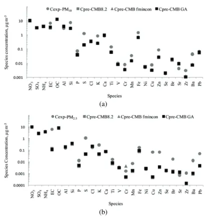
Comparison between the experimental and calculated concentrations of 26

species in PM

10

and PM

2.5

analyzed through estimates of the source contribution

from the three respective CMB approaches in the Fresno (Fig. 3) and Bakersfield

(a)

(b)

Fig. 3. Experimental concentrations (cexp) and the concentrations of species predicted by CMB8.2, CMB–fmincon and CMB–GA (c_pre-CMB8.2, c_{pre-CMB-fmincon} and c_pre-CMB-GA,

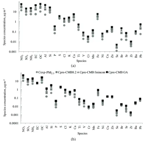
(Fig. 4) data revealed possible deviations of the concentrations species from the

real data. Since the genetic algorithm approach revealed large percentage mass

(both Fresno and Bakersfield) with low

χ

2

_{and a better}

_R

2

_{value, accurate}

concentrations of the species are predicted than the respective values obtained

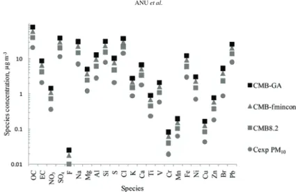
from CMB–fmincon and CMB8.2. The experimental and predicted species

concentration data obtained for Portland, Oregon PM

10

is shown in Fig. 5. The

least errors between

C

exp

and

C

pre

were observed for the data analyzed by CMB–

–GA than the data analyzed by CMB–fmincon or CMB8.2.

(a)

(b)

Fig. 4. Experimental concentrations (c_exp) and concentrations of species predicted by CMB8.2, CMB–fmincon and CMB–GA (cpre-CMB8.2, cpre-CMB-fmincon and cpre-CMB-GA,

Fig. 5. Experimental concentrations (cexp) and concentrations of species predicted by CMB8.2, CMB–fmincon and CMB–GA (c_pre-CMB8.2, c_{pre-CMB-fmincon} and c_pre-CMB-GA,

respectively) in PM10 from Portland, OR, data.

CONCLUSIONS

The output of chemical mass balance model gives the contribution of each

source type represented by a composition to the total mass, as well as to each

chemical species in the receptor concentration. A comparison of CMB receptor

models was performed to understand the efficiency in source contribution

through various optimization techniques. The source profile uncertainty and

rec-eptor concentration uncertainties were used in the CMB8.2 software tool

devel-oped by USEPA. Optimized source contributions were obtained by CMB–GA

and CMB–fmincon. The best estimate of the source contributions from the

con-verged solution through CMB–GA was possible by a large number of

gener-ations. The source contributions obtained from the CMB8.2 deviated more in

comparison with those obtained from the CMB–fmincon and CMB–GA because

of the constrained optimization by ‘fmincon’ and GA solvers. The model

accur-acy was validated by various performance measures such as

R

2

, χ

2

and

percent-age mass for the three respective CMB approaches. Very high correlations

between

c

_pre

and

c

_exp

were obtained from CMB–GA for the Bakersfield data

(0.81 and 0.83) than from CMB–fmincon and CMB8.2.

χ

2

_{(0.36, 0.66 and 0.65,}

0.43) and percentage mass (67.36 , 55.03 and 94.24 %, 74.85 %) from the

CMB–GA model illustrated more accurate data for PM

10

and PM

2.5

from Fresno

and Bakersfield. The methodology was followed with Portland, OR, PM

10

data

that also resulted in the best fit from CMB–GA with R

2

_,

χ

2

_{and percentage mass}

SUPPLEMENTARY MATERIAL

The execution of CMB by ‘fmincon’ solver in MATLAB R2008a, Fig. S-1, execution of the genetic algorithm code, Fig. S-2, details of the CMB–GA method and source contributions for the analyzed species in PM10 and PM2.5 obtained using CMB8.2, CMB–fmincon and CMB–GA for the Fresno, Bakersfield and Oregon stations, Figs. S-3–S-5, are available electronically from http://www.shd.org.rs/JSCS/, or from the corresponding author on request.

Acknowledgement.The authors are very grateful to the editors and reviewers for their valuable comments and suggestions, which helped to improve the quality of the manuscript.

И З В О Д

ЕВАЛУАЦИЈАОПТИМИЗАЦИЈЕМЕТОДЕЗАРЕШАВАЊЕМОДЕЛАХЕМИЈСКОГ БИЛАНСАМАСЕ

N. ANU, S. RANGABHASHIYAM, RAHUL ANTONY и N. SELVARAJU Department of Chemical Engineering, National Institute of Technology Calicut

Kozhikode-673601, Kerala, India

Модел хемијског биланса масе (CMB) се користи да би се одредили доприноси изворачестица (пречникамањиход 10 и 2,5 μm) уанализиквалитетаваздуха. Поређење доприносаизвораодређенихнаосновутри CMB модела (CMB 8.2, CMB fmincon и CMB– –GA) је вршено коришћењем оптимизационих техника, као што су ‘fmincon’ (CMB– –fmincon) игенеричкиалгоритам (CMB–GA), упрограмскомпакету MATLAB. Предло -жени приступ је потврђен коришћењем података San Joaquin Valley Air Quality Study

(SJVAQS) California Fresno и Bakersfield PM₁₀ и PM_2,5, као и Oregon PM₁₀. Допринос извораодређениз CMB–GA јебиобољипопитањуинтерпретацијеизвора, упоређењуса CMB 8.2 i CMB–fmincon. Валидацијапоузданоститри CMB приступајевршенакориш -ћењемследећих параметара: R2_{, редукованиχ}2_{ипроценатмасе. R}2 _{(0,90, 0,67 и 0,81,}

0,83), χ2 (0,36, 0,66 и 0,65, 0,43) и проценат масе (67,36, 55,03 и 94,24 %, 74,85 %) тестовиза CMB–GA супоказалидобрукорелацијуза PM10и PM2,5 Fresno и Bakersfield

податке. Да биседошлодо коначнеодлуке, предложенаметодологијајебила приме -њенана Portland, OR, PM10податкесанајбољимслагањемсаR2 (0,99), χ2 (1,6) ипро

-ценатмасе (94,4 %) из CMB–GA. Збогтогајеовоиспитивањепоказалода CMB сагене -ричкималгоритмомоптимизацијеимабољустабилностуодређивањудоприносаизвора.

(Примљено 14. новембра 2013, ревидирано 31. марта, прихваћено 18. маја 2014)

REFERENCES

1. A. O. M. Carvalho, M. C. Freitas, Procedia Environ. Sci. 4 (2011) 184 2. X. Zhang, W. Chen, C. Ma, S. Zhan, Sci. Total Environ. 449 (2013) 168 3. A. Kristin, W. Shuxiao, Sci. Total Environ. 481 (2014) 186

4. S. Yatkin1, A. Bayram, Chemosphere71 (2008) 685

5. B. Srimuruganandam1, S. M. Shiva Nagendra, Sci. Total Environ. 433 (2012) 8

6. Z. Huarong, X. Beicheng, F. Chen, Z. Peng, S. Shili, Sci. Total Environ. 417–418 (2012) 45 7. M. Viana1, M. Pandolfi, M. C. Minguillon, X. Querol, A. Alastuey, E. Monfort, I.

Celades, Atmos. Environ. 42 (2008) 3820

8. C. A. Belis, F. Karagulian, B. R. Larsen, P. K. Hopke, Atmos. Environ. 69 (2013) 94 9. A. Lukewille, I. Bertok, M. Amann, J. Cofala, F. Gyarfas, M. Johansson, Z. Klimont, E.

11. R. C. Henry, C. W. Lewis, P. K. Hopke, H. J. Williamson, Atmos. Environ. 18 (1984) 1507 12. J. C. Chow, J. G. Watson, Energy Fuels16 (2002) 222

13. B. R. Larsen, H. Junninen, J. Monste, M. Viana, P. Tsakovski, R. M. Duvall, G. A. Norris, X. Querol, The Krakow Receptor Modelling Intercomparison Exercise Rep. JRC Scientific and Technical Reports, EUR 23621 EN 2008, Ispra, 2008

14. M. Pandolfi, M. Viana, M. C. Minguillon, X. Querol, A. Alastuey, F. Amato, I. Celades, A. Escrig, E. Monfort, Atmos. Environ. 42 (2008) 9007

15. S. Kong, B. Han, Z. Bai, L. Chen, J. Shi, Z. Xu, Sci. Total Environ. 408 (2010) 4681 16. S. Yatkin, A. Bayram, Environ. Monit. Assess. 167 (2010) 125

17. J. H. Seinfeld, S. N. Pandis, Atmospheric chemistry and physics from air pollution to climate change, 2nd _{ed., Wiley, Hoboken, NJ, 2006, p. 1136}

18. L. W. A. Chen, J. G. Watson, J. C Chow, D. W. DuBois, L. Herschberger, Atmos. Environ. 44 (2010) 4908

19. W. F. Christensen, Atmos. Environ. 38 (2004) 4305

20. W. F. Christensen, R. F. Gunst, Atmos. Environ. 38 (2004) 733 21. G. Argyropoulos, C. Samara, Environ. Modell. Softw. 26 (2011) 469

22. G. Argyropoulos, Th. Grigoratos, M. Voutsinas, C. Samara, Environ. Sci. Pollut. Res. Int.

20 (2013) 7214

23. H. S. Javitz, J. G. Watson, N. Robinson, Atmos. Environ. 22 (1988) 2309 24. H. Cheng, A. Sandu, Environ. Modell. Software24 (2009) 917

25. T. C. Coulter, EPA-CMB8. User’s Manual, EPA-452/R-04-011 United States Environ-mental Protection Agency, Research Triangle Park, NC, 2004

26. N. Selvaraju, S. Pushpavanam, N. Anu, Environ. Monit. Assess. 185 (2013) 10115 27. N. Anu, S. Rangabhashiyam, N. Selvaraju, S. Pushpavanam, J. Sci. Ind. Res. 72 (2013) 754 28. J. C. Chow, J. G. Watson, D. H. Lowenthal, P. A. Solomon, K. L. Magliano, S. D. Ziman,

L. W. Richard, Atmos. Environ., A 26 (1992) 3335

29. J. C. Chow, J. G. Watson, D. H. Lowenthal, P. A. Solomon, K. L. Magliano, S. D. Ziman, L. W. Richard, Aerosol Sci. Technol. 18 (1993) 105

30. J. G. Watson, J. A. Cooper, J. J. Huntzicker, Atmos. Environ. 18 (1984) 1347

31. A. Chipperfield, P. Fleming, H. Pohlheim, C. Fonseca, Genetic Algorithm TOOLBOX User’s Manual, version 1.2, University of Sheffield, Sheffield, https://www.shef-field.ac.uk/polopoly_fs/1.60188!/file/manual.pdf (accessed in Feb, 2015)

32. K. F. Ho, S. C. Lee, J. C. Chow, J. G. Watson, Atmos. Environ. 37 (2003) 1023