On-line and off-line data assimilation of palaeoclimate proxy data into a GCM using ensemble member selection

(1)

CPD

10, 3449–3482, 2014

On-line and off-line data assimilation

A. Matsikaris et al.

Title Page

Abstract Introduction

Conclusions References

Tables Figures

◭ ◮

Back Close

Full Screen / Esc

Printer-friendly Version

Interactive Discussion

Discussion

P

a

per

|

Discus

sion

P

a

per

|

Discussion

P

a

per

|

Discussion

P

a

per

|

Clim. Past Discuss., 10, 3449–3482, 2014 www.clim-past-discuss.net/10/3449/2014/ doi:10.5194/cpd-10-3449-2014

This discussion paper is/has been under review for the journal Climate of the Past (CP). Please refer to the corresponding final paper in CP if available.

On-line and o

_ff

-line data assimilation of

palaeoclimate proxy data into a GCM

using ensemble member selection

A. Matsikaris1,2, M. Widmann1, and J. Jungclaus2

1

University of Birmingham, Edgbaston, Birmingham B15 2TT, UK

2

Max-Planck-Institute for Meteorology, Hamburg, Germany

Received: 28 July 2014 – Accepted: 8 August 2014 – Published: 22 August 2014 Correspondence to: A. Matsikaris (axm368@bham.ac.uk)

(2)

CPD

10, 3449–3482, 2014

Title Page

Tables Figures

◭ ◮

Back Close

Full Screen / Esc

Discussion

P

a

per

|

Discus

sion

P

a

per

|

Discussion

P

a

per

|

Discussion

P

a

per

|

Abstract

Different ensemble-based data assimilation (DA) approaches for palaeoclimate recon-structions have been recently followed, but no systematic comparison among them has been attempted. We compare an o_ff-line and an on-line ensemble-based method, with the testing period being the 17th century, which led into the Maunder Minimum. We use

5

a low-resolution version of Max Planck Institute for Meteorology’s model MPI-ESM, to assimilate the PAGES 2K continental temperature reconstructions. In the off-line ap-proach the ensemble for the entire simulation period is generated first and then the ensemble is used in combination with the empirical information to produce the analy-sis. In contrast, in the on-line approach the ensembles are generated sequentially for

10

sub-periods based on the analysis of previous sub-periods. Both schemes perform bet-ter than the simulations without DA. The on-line method would be expected to perform better if the assimilation led to states of the slow components of the climate system that are close to reality and the system had sufficient memory to propagate this informa-tion forward in time. In our comparison, which is based on analysing correlainforma-tions and

15

differences between the analysis and the proxy-based reconstructions, we find similar skill for both methods on continental and the hemispheric scales. This indicates either a lack of control of the slow components in our setup or a lack of information propa-gation on decadal timescales. Although the skill is similar and the on-line method is more difficult to implement, the temporal consistency of the analysis in on-line method

20

makes it in general preferable.

1 Introduction

Reconstructing the climate of the past is crucial for quantifying and understanding natural climatic change, which in turn is essential for detecting anthropogenic climate change, as well as for the validation of climate models that are used to provide future

25

(3)

esti-CPD

10, 3449–3482, 2014

Title Page

Tables Figures

◭ ◮

Back Close

Full Screen / Esc

Discussion

P

a

per

|

Discus

sion

P

a

per

|

Discussion

P

a

per

|

Discussion

P

a

per

|

mate low-frequency variability, reconstructions based on climate proxy data or numer-ical simulations are used for this purpose. However, both approaches are associated with substantial uncertainties. In principle, the best state estimates can be expected by employing data assimilation (DA) techniques, which systematically combine the empir-ical information from proxy data with the representation of the processes that govern

5

the climate system given by climate models. Although DA is a very mature field in nu-merical weather prediction, the specific problem in palaeoclimatology is different and the methods cannot be directly transferred (e.g. Widmann et al., 2010; Hakim et al., 2013). DA is an emerging research area and can be considered as one of the key challenges in palaeoclimatology.

10

There are two types of proxy-based reconstructions, those for large-scale, e.g. con-tinental or hemispheric averages (e.g. Moberg et al., 2006; PAGES 2K Consortium, 2013) and spatial field reconstructions (e.g. Briffa, 2000; Crowley and Lowery, 2000; Jones and Mann, 2004; Mann et al., 2008). Proxy-based estimates of climate vari-ability contain considerable uncertainties: different proxies usually represent different

15

seasons, different statistical methods used in the reconstructions lead to different re-sults, and non-climatic factors influence the proxies. Moreover, the poor spatial cov-erage of the climate proxies leads to errors in hemispheric or continental means and even larger errors in full-field reconstructions. The climate states provided by standard model simulations are spatially complete and provide an independent estimate which

20

can be checked for consistency with the proxies, on both large and regional scales. However, the simulations also have errors, e.g. systematic model biases and errors in the climate forcings or in the response to them. Additionally, interannual to decadal tem-perature variations have a large random, non-forced component and thus agreement of simulations and observations is very unlikely on these timescales. The forcings do

25

(4)

CPD

10, 3449–3482, 2014

Title Page

Tables Figures

◭ ◮

Back Close

Full Screen / Esc

Discussion

P

a

per

|

Discus

sion

P

a

per

|

Discussion

P

a

per

|

Discussion

P

a

per

|

Data assimilation combines the two previous methods to find estimates that are both consistent with the empirical knowledge and with the dynamical understanding of the climate system. It uses the empirical data after the construction of the model to either estimate, correct or select the system state (e.g. Hakim et al., 2013; Bronnimann et al., 2013), or to systematically improve some model parameters (e.g. Annan et al., 2013).

5

Here, we consider the case of state estimation, where DA aims to capture the real-world random, non-forced variability in a simulation and to provide information for variables for which no empirical estimates exist.

Attempts to assimilate proxy data into models include different approaches, such as the selection of ensemble members, forcing singular vectors, and pattern nudging

10

(e.g. Widmann et al., 2010). Ensemble member selection techniques, like the one im-plemented here, are based on the selection of simulations from an ensemble that are closest to the empirical evidence on climate. A general advantage of these techniques is that they are easy and straightforward to implement, and they are the most fre-quently used methods by the community. Goosse et al. (2006) were the first to use this

15

method for palaeoclimate research, employing a simplified global 3-D climate model. An updated version was employed by Goosse et al. (2010), using a more advanced 3-D Earth-System Model of Intermediate Complexity (EMIC), along with a set of 56 proxy series derived from a comprehensive compilation of Mann et al. (2008). In the first case, the best model analog was selected by comparing the simulations with

20

proxy-based temperature reconstructions after the completion of the simulations, an approach called off-line DA. In the second case a new ensemble was generated at each step of the assimilation procedure, starting from the best simulation selected for the previous period, an approach called on-line DA. The revised method offered dy-namical consistency between best model analogs of different periods, while the former

25

(5)

CPD

10, 3449–3482, 2014

Title Page

Tables Figures

◭ ◮

Back Close

Full Screen / Esc

Discussion

P

a

per

|

Discus

sion

P

a

per

|

Discussion

P

a

per

|

Discussion

P

a

per

|

In addition to the above method, where a single simulation having the best fit to the data is chosen during the assimilation (“degenerate particle filter”), another approach employs weights for each member of the ensemble, calculated after the comparison with the proxies and generating a probabilistic posterior distribution (“particle filter”). The technique was applied by Annan and Hargreaves (2012), who used a simple

likeli-5

hood weighting algorithm and involved off-line assimilation, performing thus all the DA after the completion of the ensemble integration. In the “particle filter” methods, more than one member proceeds to the next assimilation step after the first filtering. The most unlikely ensemble members (particles) are being stopped and the highly likely particles are being copied proportionally to their likelihood. The same “probabilistic

10

posterior distributions” technique was used by Goosse et al. (2012). The outcomes of the approach led to distributions with larger overlaps with the proxy-based recon-struction. The method has also been used by Mairesse et al. (2013) to reconstruct the climate of the mid-Holocene (6 kyr BP).

Other ensemble-based DA approaches include the use of the Kalman filter including

15

the explicit treatment of time-averaged observations. The off-line approach of DA was advanced by Bhend et al. (2012), through the assimilation of proxy data into a high-resolution general circulation model (GCM). The ensemble square root filter (EnSRF), a variant of the ensemble Kalman filter, was used to update the ensembles with cli-mate proxy information. An o_ff-line scheme was used at the DA, since the use of an

20

atmosphere-only GCM rather than a coupled atmosphere–ocean GCM left no possi-bility for information propagation on long timescales. In other words, an on-line DA scheme would not have benefitted the reconstruction skill, apart from leading to tem-poral consistency of the analysis. Dirren and Hakim (2005) examined the case where only time-averaged observations are available. Their algorithm constitutes a natural

25

(6)

cli-CPD

10, 3449–3482, 2014

Title Page

Tables Figures

◭ ◮

Back Close

Full Screen / Esc

Discussion

P

a

per

|

Discus

sion

P

a

per

|

Discussion

P

a

per

|

Discussion

P

a

per

|

mate variability related to the palaeoproxies. In order to identify initial conditions, an ensemble Kalman filter technique was applied to the two models.

An advantage of the on-line compared to the off-line ensemble-based DA methods is the temporal consistency of the simulated states. The off-line approach on the other hand is computationally less complicated and can also be computationally cheaper

5

if one uses simulations that already exist. The question we address in this paper is whether the on-line reconstruction is closer to the proxy-based reconstructions com-pared to the off-line version. This depends on the memory of the slow components of the climate system, such as the ocean. If these propagate the information contained in the assimilated proxy data forward in time on decadal timescales, the on-line approach

10

is expected to perform better. If, on the other hand, the chaotic nature of the system dominates and the predictability of the system is limited, the computationally easier off -line method would be sufficient. GCMs exhibit up to decadal predictability in the North Atlantic and the ocean predictability can in turn lead to atmospheric predictability. The extent of decadal predictability and the relevant mechanism behind are not yet clear

15

and many studies have recently been performed on these topics (e.g. Steiger et al., 2014; Hawkins and Sutton, 2009a, b; Keenlyside and Ba, 2010).

In this paper, we compare two ensemble-based DA approaches, an off-line and an on-line method, to reconstruct the climate for the period 1600–1700 AD, which led into the Maunder Minimum. This is a period for which many proxy studies and model

simu-20

lations exist, and which is interesting due to the large temperature variations exhibited in the transition to the prolonged cold period of the Maunder Minimum (about 1645 AD to 1715 AD). We employ ensemble simulations with the Max Planck Institute for Meteo-rology’s General Circulation Model MPI-ESM, and specifically a low-resolution version of the MPI CMIP5 model. The proxy temperature reconstructions of the PAGES 2K

25

project are used in our assimilation.

(7)

CPD

10, 3449–3482, 2014

Title Page

Tables Figures

◭ ◮

Back Close

Full Screen / Esc

Discussion

P

a

per

|

Discus

sion

P

a

per

|

Discussion

P

a

per

|

Discussion

P

a

per

|

a first comparison of them, while in Sect. 4, we draw conclusions and discuss the ben-efits of each approach.

2 Experimental design

2.1 Model simulations

We used the Max Planck Institute for Meteorology Earth System Model (MPI-ESM),

5

comprising of the general circulation models ECHAM6 (Stevens et al., 2013) for the atmosphere and MPIOM (Marsland et al., 2003) for the ocean. ECHAM6 was run at T31 horizontal resolution (3.75◦

×3.75◦), with 31 vertical levels, resolving the atmosphere up to 10 hPa. MPIOM was run at a horizontal resolution of 3.0◦_{(GR30) and 40 vertical} levels. The OASIS3 coupler was used to couple the ocean and the atmosphere daily

10

without flux corrections. The land surface model was JSBACH (Raddatz et al., 2007) and no ocean biogeochemistry model was employed. The model is a low-resolution version of the model used for the Coupled Model Intercomparison Project Phase 5 (CMIP5) simulations.

The simulations described here are based on a simulation covering the last

millen-15

nium (850–1849 AD) following the “past1000” protocol of the Paleo Model Intercom-parison Project Phase 3 (Schmidt et al., 2011). Prescribed external forcing factors are reconstructed variations of total solar irradiance (Vieira et al., 2011), volcanic aerosols (Crowley and Unterman, 2012), concentrations of the most important greenhouse gases (Schmidt et al., 2011), and anthropogenic land-cover changes (Pongratz et al.,

20

2008). A long control simulation with constant pre-industrial (1850 AD) boundary con-ditions was also conducted and the past1000 simulation was started after a 700 year long spin-up with constant 850 AD boundary conditions.

The high computational cost restricted us to running 10 ensemble members for each experiment. This choice is consistent with Bhend et al. (2012) who found that

ensem-25

(8)

CPD

10, 3449–3482, 2014

Title Page

Tables Figures

◭ ◮

Back Close

Full Screen / Esc

Discussion

P

a

per

|

Discus

sion

P

a

per

|

Discussion

P

a

per

|

Discussion

P

a

per

|

the proxies, and that considerable skill in regions close to the assimilated data can be found for ensembles of 15 members or more, while larger sizes are needed for areas further away. The ensemble members have been generated by slightly varying values of an atmospheric diffusion parameter. The method leads to a fast divergence of the different simulations and an adequate ensemble spread, not only in surface variables

5

like the 2m or sea-surface temperature, but also in deeper ocean variables, such as the AMOC – Atlantic meridional overturning circulation. The selected ensemble gener-ation method does not directly introduce any disturbance in the ocean, which may limit the capability of the assimilation scheme. For this reason, a di_fferent way of generating ensembles was also tested, namely the lagged-ocean initialization method, generating

10

the ensemble members by using different ocean initial conditions, based on different dates close to the original starting date of the generation. The similarity in the output of the two methods however, and the fact that the lagged-ocean initialization method could produce unobserved forcings for some simulations, led us to choose the atmosphere-only disturbance.

15

2.2 Proxy datasets

For our assimilation procedure, we used the “2k Network” of the IGBP Past Global Changes (PAGES) proxy datasets. The PAGES project used a global set of proxy records and produced temperature reconstructions for seven continental-scale regions (PAGES 2K Consortium, 2013). The dataset covers different periods during the last

20

millennium for each continent, and specifically the years 167–2005 AD for Antarc-tica, 1–2000 AD for the Arctic, 800–1989 AD for Asia, 1001–2001 AD for Australasia, 1–2003 AD for Europe, 480–1974 AD for North America and 857–1995 AD for South America. It has been produced by nine regional working groups, who identified the best proxy climate records for the temperature reconstruction within their region, using

25

(9)

CPD

10, 3449–3482, 2014

Title Page

Tables Figures

◭ ◮

Back Close

Full Screen / Esc

Discussion

P

a

per

|

Discus

sion

P

a

per

|

Discussion

P

a

per

|

Discussion

P

a

per

|

et al., 2008, 2009), or regression-based techniques for the predictors, including prin-cipal component pre-filters or distance weighting (PAGES 2K Consortium, 2013). The dataset of individual proxies consists of 511 time series that include ice cores, tree rings, pollen, speleothems, corals, lake and marine sediments as well as historical documents of changes in biological or physical processes. The reconstructions have

5

annual resolution, apart from North America, which is resolved in ten- and thirty-year periods.

2.3 Selection of the best ensemble members

We simulated the period 1600–1700 AD using the standard forcings for this period. The initial conditions were those of the last day of the year 1599 AD, taken from a

tran-10

sient forced simulation starting in 850 AD. We performed ensemble experiments of 100 year duration. In the off-line experiment, in the first year (1600 AD), the ten ensem-ble members used slightly different values of an atmospheric diffusion parameter. For each member, the simulation period was divided into 10 year intervals, and the decadal means of the 2m temperature were calculated for each of the Northern Hemisphere

15

continents. Using a root mean square (RMS) error-based cost function, the model outputs were compared to the proxy-based continental temperature reconstructions, averaged over the respective 10 year periods. The ensemble member that minimized the cost function in each decade was selected as the best simulation for that period. The same process was followed for all the decades within the analysis period, so that

20

in the end we obtained the analysis, by merging the best members of each decade. The selection of the “optimal” simulation of the ensemble for each decade of the simulation period was done after the calculation of the following cost function:

CF(t₎₌

v u u t

k

X

i₌1

Tk

mod(t)−T

k

prx(t) 2

(1)

(10)

CPD

10, 3449–3482, 2014

Title Page

Tables Figures

◭ ◮

Back Close

Full Screen / Esc

Discussion

P

a

per

|

Discus

sion

P

a

per

|

Discussion

P

a

per

|

Discussion

P

a

per

|

wherek _{are the Northern Hemisphere continents, namely the Arctic, Asia, Europe and}

North America,Tk

mod(t) is the standardized modelled decadal mean of the temperatures in each Northern Hemisphere continent andT_prxk ₍t_{) is the standardized proxy-based}

re-construction for the decadal mean of the temperatures in each Northern Hemisphere continent. The algorithm filters out the particles that are considered poor

representa-5

tions of the actual state, by throwing away the ones that are less consistent with the proxies and promoting the best fitting particle. We include the data of the Northern Hemisphere alone in the cost function, in an effort to reduce the degrees of freedom of the system and make it easier to find good analogues with our small ensemble size. Moreover, the Southern Hemisphere is affected by bigger uncertainties and is

recon-10

structed by less dense proxy networks.

The reason for basing the cost function on standardized simulated and proxy-based temperatures is to remove systematic biases between the model and the proxy-based reconstructions, and to avoid that continental temperatures with di_ffering variance do not contribute equally to the analysis. The standardized model and proxy time-series

15

were calculated by subtracting the 850–1850 AD means of the model output and the proxies from the 1600–1700 AD raw model output and proxies respectively, and dividing by the respective standard deviations, based on the decadal averages for the 850– 1850 AD period. The datasets were not weighted according to the size of the different regions, as we consider all continents to be equally important. We also decided against

20

weighting on the base of the errors of the proxy datasets, as the different methods followed by each of the PAGES 2K groups make the errors not directly comparable. Moreover, the errors of the continental reconstructions are of similar order and thus error weighting would only have a small effect.

In the on-line experiment, a ten-member ensemble was generated for the first year

25

(11)

CPD

10, 3449–3482, 2014

Title Page

Tables Figures

◭ ◮

Back Close

Full Screen / Esc

Discussion

P

a

per

|

Discus

sion

P

a

per

|

Discussion

P

a

per

|

Discussion

P

a

per

|

the off-line method, the selected member for that period, i.e. the one that minimized the cost function, was used as the initial condition for the subsequent simulation. A new en-semble consisting of 10 members was performed for the second decade, starting from the previous best member’s final conditions and having slightly varying values of the atmospheric diffusivity parameter in the different members. The same procedure was

5

repeated until the year 1700 AD

The comparison of the two experiments is based on the proximity to the proxy-based reconstructions. We note however that it is not the aim of DA to exactly reproduce the assimilated empirical information, since these have errors. Ideally, a validation of different DA methods would be based on a comparison with the true and spatially

10

complete temperature field, but as this is not available, a validation based on proximity to the assimilated information is a useful first step to investigate whether the on-line and off-line approaches perform differently.

3 Results and discussion

We assimilate the PAGES 2K temperature reconstruction for the period 1600 AD to

15

1700 AD, which led into the Maunder Minimum. The Maunder minimum (1645 AD to 1715 AD) was characterized by a large reduction in the number of sunspots and hence a reduction in solar radiation, and corresponds to the middle part of the Little Ice Age. The PAGES 2K reconstructions exhibit a cooling in all the continents except Antarctica for this period, being in agreement with previous studies. Fossil coral evidence

sug-20

gests that El Nino-like conditions prevailed during the 17th century (Jones and Mann, 2004).

Having a good chance to find a close analogue of an atmospheric state requires a large number of ensemble members, if the state space has a high dimension. Van Den Dool (1994) found that to find an accurate analogue for daily data over a large

25

(12)

li-CPD

10, 3449–3482, 2014

Title Page

Tables Figures

◭ ◮

Back Close

Full Screen / Esc

Discussion

P

a

per

|

Discus

sion

P

a

per

|

Discussion

P

a

per

|

Discussion

P

a

per

|

braries of only 10–100 years of data, analogues can be found only in just 2 or 3 degrees of freedom (e.g. Bretherton et al., 1999). In our case, by using only the continental av-erages of the Northern Hemisphere as targets for the assimilation process, we have a low number of degrees of freedom for our cost function (less than 3). This makes the detection of a good analogue much more likely with our small ensemble size of

5

10 members. The performance of the two schemes was assessed by computing the correlation and the root-mean-square (RMS) error for each Northern Hemisphere (NH) continent between the simulated and the proxy-based reconstructions of the 2 m air temperatures.

3.1 Validation of the off-line DA scheme 10

Despite the fact that the cost function for the selection of the best members was based on standardized data, we demonstrate the performance of the two schemes using the non-standardized, but unbiased model output (absolute anomalies). This is because the latter represents the actual assimilated temperatures that come out of the model, which can be compared with other studies. The validation of the off-line DA scheme

15

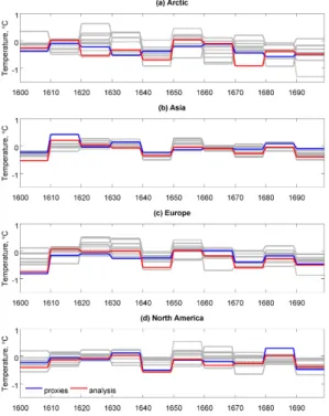
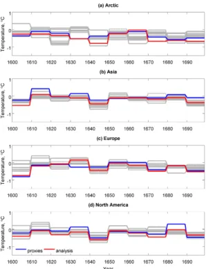
shows a clear improvement of the simulated reconstruction for the period under con-sideration, presenting higher correlations between model and proxies for all the conti-nents of the Northern Hemisphere and lower root mean square errors for the analysis compared to the individual members. The analysis was formed by merging the best members of each decade together. Figure 1 shows the Northern Hemisphere

conti-20

nents’ decadal mean temperatures for the 17th century for the 10 ensemble members, the proxy-based reconstructions and the off-line DA analysis. The analysis for all the NH continents is closer to the proxies than any of the individual ensemble members. This result is not trivial, as the cost function only minimizes the RMS error with respect to all NH continents.

25

(13)

CPD

10, 3449–3482, 2014

Title Page

Tables Figures

◭ ◮

Back Close

Full Screen / Esc

Discussion

P

a

per

|

Discus

sion

P

a

per

|

Discussion

P

a

per

|

Discussion

P

a

per

|

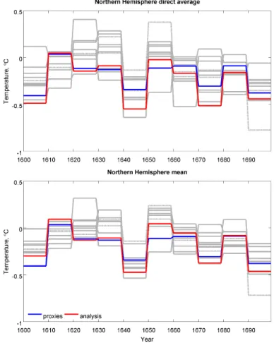
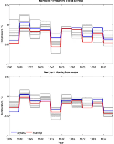
makes use of the same sea-land masks and seasonal representativity as the ones employed by the proxy reconstructions. Hence, it is directly comparable to the proxy datasets, which are only available as continental means. The NH mean on the other hand is the true spatial average temperature of the whole Northern Hemisphere. We show this time-series as it is the usual mean temperature given in most climate studies,

5

despite the fact that in our comparison it not the direct equivalent of the proxy-based reconstructions (the proxy time-series in the two cases are the same). The correlations between the analysis and the proxies are relatively high for all the NH continents (0.56 for the Arctic, 0.78 for Asia, 0.79 for Europe and 0.89 for North America). Since the cost function includes all the NH continents, the correlation is maximum for the Northern

10

Hemisphere direct average (0.94), while the correlation for the Northern Hemisphere mean is also high (0.92). These values are much higher than the correlations of the in-dividual members with the proxies, and also higher than the correlation of the ensemble mean with the proxies (0.73).

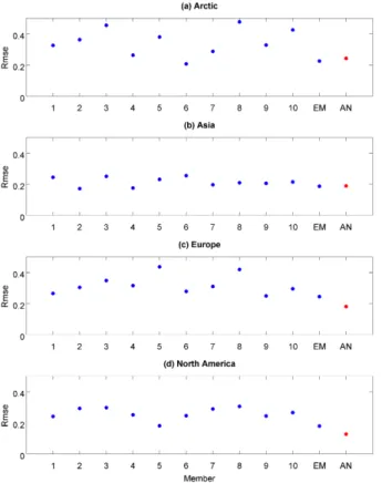
The RMS error of the simulated time-series for each continent provide a

quantifica-15

tion of the local agreement between the model and the proxy-based reconstructions. It is calculated based on the decadal mean di_fferences of the model and the proxy time-series for each continent. Figure 3 shows the RMS errors for the individual members, the ensemble mean and the analysis of the four Northern Hemisphere continents. The RMS errors are either minimal or among the lowest for the analysis compared to all

20

other members. The result is even more obvious when considering the RMS errors for the direct average of the Northern Hemisphere, where the analysis had clearly the lowest value (not shown). The fact that the RMS error of the ensemble mean is lower than the error of most of the individual members indicates the influence of forcings in some continents. However, a better estimate can be still obtained from the DA

analy-25

sis, which means that internal variability is important too, especially for Europe, North America and the direct average of the NH.

(14)

CPD

10, 3449–3482, 2014

Title Page

Tables Figures

◭ ◮

Back Close

Full Screen / Esc

Discussion

P

a

per

|

Discus

sion

P

a

per

|

Discussion

P

a

per

|

Discussion

P

a

per

|

using the absolute anomalies and presented above. For the Southern Hemisphere, it is more meaningful to assess the performance of the method using the standard-ized data, as the RMS error only has a meaning with this approach. Not using the standardized outputs in this case would result in non-comparable scales because of the different standard deviations between model and proxies. In contrast to the good

5

skill of the scheme in the Northern Hemisphere, the agreement between the anal-ysis for the Southern Hemisphere (SH) and the proxy-based reconstructions is not good, as expected from the fact that SH data are not included in the cost function. It is noteworthy that the PAGES 2K record for Antarctica shows less cooling than the NH records during the seventeenth century. As the NH cooling during this period has been

10

mainly attributed to solar and volcanic forcings (Jones and Mann, 2004), this indicates a weaker sensitivity of Antarctica to these forcings, presumably due to the large fraction of ocean in the SH and the high albedo of Antarctica.

3.2 Validation of the on-line DA scheme

The on-line DA scheme was also successful, improving the skill of the analysis

time-15

series compared to the individual members. However, the scheme presented very sim-ilar correlations between the DA analysis and the proxy-based reconstructions with the ones found with the o_ff-line approach, and no major improvements to the RMS errors, both on the continental scales and the direct averages. The NH continents’ decadal mean temperatures for the 17th century, for the 10 ensemble members, the

proxy-20

based reconstructions and the on-line DA analysis are displayed in Fig. 4 and show the good proximity of the analysis to the empirical reconstruction. Even better agree-ment is exhibited by the direct average of the four Northern Hemisphere continents and the Northern Hemisphere mean, as illustrated in Fig. 5. Validation of the absolute anomalies reveal that correlations between analysis and proxies are high for all the

25

(15)

CPD

10, 3449–3482, 2014

Title Page

Tables Figures

◭ ◮

Back Close

Full Screen / Esc

Discussion

P

a

per

|

Discus

sion

P

a

per

|

Discussion

P

a

per

|

Discussion

P

a

per

|

DA scheme, the above values are much higher than the correlations of any individual member with the proxies, as well as higher than the correlation of the ensemble mean with the proxies (0.67).

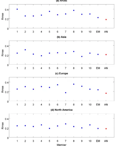
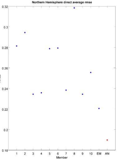
The RMS errors for the analysis of the NH continents are among the lowest com-pared to the different members, as shown by Fig. 6. This is also the case for the direct

5

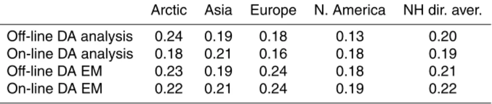
average of the NH continents and the NH mean, to an even greater extent compared to the respective individual members (Fig. 7). Specifically, the RMS errors between the analysis and the proxies in the on-line DA scheme are 0.18 for the Arctic, 0.21 for Asia, 0.16 for Europe and 0.18 for North America. The RMS error for the direct average of the four Northern Hemisphere continents is 0.19.

10

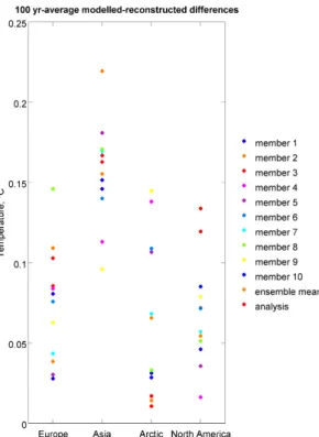
The construction of our cost function on the base of decadal mean temperatures of the NH, means that the analysis is not expected to be more skilful than the individual members when considering the hundred-year average. The 17th century average tem-peratures for the NH continents are presented in Fig. 8, and indeed do not exhibit the best agreement between the analysis and the proxy-based reconstructions in all the

15

regions, although this is the case for some continents (the Arctic and Europe).

3.3 Comparison of the two DA schemes

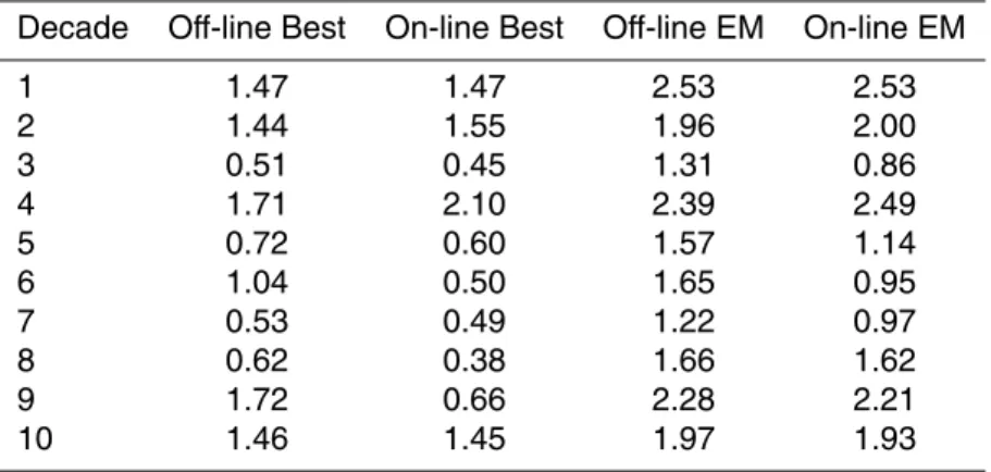
As previously noted, both DA schemes perform better than the simulations without DA. Not much difference appears between the two of them. In seven out of the 10 decades of the testing period, a lower cost function for the best member and the ensemble mean

20

is found when using the on-line method, but the di_fferences with the o_ff-line approach are very small (Table 1), not allowing any robust statements about one method be-ing better than the other. The respective ensemble mean (EM) cost functions are also shown in the table. Table 2 shows the Northern Hemisphere RMS errors between sim-ulations and proxy-based reconstructions for the analysis and the ensemble mean of

25

(16)

CPD

10, 3449–3482, 2014

Title Page

Tables Figures

◭ ◮

Back Close

Full Screen / Esc

Discussion

P

a

per

|

Discus

sion

P

a

per

|

Discussion

P

a

per

|

Discussion

P

a

per

|

17th century are displayed in Fig. 9, where none of the two analyses can be deemed as better in following the proxy-based reconstruction. The proximity of the analyses of the two methods can also be seen in Fig. 10. The figure displays the analyses of the on-line and the off-line DA methods for the 2 m mean temperature (anomalies w.r.t. the 1961–90 AD mean) and 500hPa geopotential height (anomalies w.r.t. the 1961–90 AD

5

mean) of the decade 1640–49 AD We see some similar patterns emerging, e.g. cool Barents Sea and warm NW Atlantic. An interesting question to answer is whether we would see differences in the performances of the two schemes if we included circula-tion indices from proxies. It could also be interesting to examine if it could be useful to include more proxy information from the ocean (e.g. the North Atlantic), to get a better

10

estimate of the ocean state.

In our setup, it appears that either no information propagation on the decadal timescales exists, or insufficient control of the ocean state affects the two DA methods. In the first case, if there is no information propagation through the slow components of the climate system, then the on-line DA scheme cannot be expected to perform better

15

than the off-line one in any setup that compares the two schemes. In the second case, di_fferent reasons may have influenced our setup, and a di_fferent setup could produce different conclusions that favour the on-line DA scheme.

A first explanation of the equal skill of the two methods would be that the decadal res-olution of the cost function indicates very little predictability in the atmosphere–ocean

20

system. The ocean predictability is not leading to significant atmospheric predictability, in other words the slow components of the climate system do not have enough memory to propagate the information contained in the assimilated proxy data forward in time on decadal timescales. Atmospheric processes in this case seem to play a more impor-tant role in the assimilation compared to the oceanic processes. Moreover, even in the

25

(17)

CPD

10, 3449–3482, 2014

Title Page

Tables Figures

◭ ◮

Back Close

Full Screen / Esc

Discussion

P

a

per

|

Discus

sion

P

a

per

|

Discussion

P

a

per

|

Discussion

P

a

per

|

However, we cannot be sure that the ocean has got no ability and memory to propa-gate the information forward on multi-year timescales. If this is not the case, a different setup could produce different conclusions that could prove the on-line DA scheme more skilful than the off-line one. Reasons for which the on-line DA is not better than the off -line DA in following the proxy-based reconstructions in our setup but could be more

5

skilful in a different setup could be various. Firstly, the insufficient control of the ocean state could be due to the small ensemble size. If the ensemble size is too small to find a member that is close to the true climatic state, there will be no added skill by propa-gating this misleading information forward in time. A second reason for the initial state of the ocean not being accurately enough determined throughout the on-line

assimi-10

lation could be that the selection of the best member was based on the atmospheric temperature state. A correct atmospheric state cannot guarantee that the ocean state is also determined correctly. A differently defined cost function, considering for example the global or direct average of the PAGES 2K continental reconstructions or different timescales could also change the performance of the two schemes. Another aspect

15

that could have influenced our approaches is the proxy datasets. The use of proxies with the minimum possible noise would give a better chance to the on-line approach to capture the true climatic state. Finally, the use of a full particle filter rather than a degen-erate one might produce a bigger ensemble spread for the ocean, giving again a better possibility to the on-line DA scheme to capture the true ocean state more closely.

20

4 Conclusions

Two main approaches have so far been employed to reconstruct the past climate: em-pirical and dynamical methods. Direct assimilation of proxy-based reconstructions into climate model simulations addresses the weaknesses of the two methods. Here, we have compared two ensemble-based DA schemes, an off-line and an on-line one, with

25

(18)

CPD

10, 3449–3482, 2014

Title Page

Tables Figures

◭ ◮

Back Close

Full Screen / Esc

Discussion

P

a

per

|

Discus

sion

P

a

per

|

Discussion

P

a

per

|

Discussion

P

a

per

|

The two DA schemes outperform the simulations without DA. The correlations between simulations and proxy-based reconstructions for the analyses of the DA schemes were higher than the correlations of the individual members, whilst the RMS errors were lower. The RMS errors of the ensemble means are lower than the errors of most of the individual members, indicating the influence of forcings in some continents,

5

but the DA analyses perform better, implying that internal variability is important too. No big difference was found between the two approaches. The majority of the cost func-tions for the best member and the ensemble mean of the on-line DA method were found to be slightly lower than the ones of the off-line DA method, but the correlations and the RMS errors, at both the continental and the hemispheric level were very close to

10

each other. The results suggest that either no information propagation on the decadal timescales exists, with insignificant predictability for the climate system, or insufficient control of the ocean state affects the two DA approaches.

These results raise the question of which approach should be preferred in the future. In some cases, since the reconstruction skill of the on-line approach is not improved

15

compared to the off-line equivalent, it would appear natural to use the less complicated o_ff-line approach to DA, especially when computationally less expensive alternatives of off-line DA schemes can be used, for example when employing simulations that already exist. The temporal consistency of the simulation is eliminated in these cases though, which does not happen in the on-line approach. In the majority of the cases,

20

and especially in the cases where the computational cost of the two methods is equal, the on-line approach should be preferred, as a result of the temporally consistent states that it provides.

Yet, we cannot be sure through these experiments whether a different setup could produce a better agreement for the on-line DA. Validation is only done with respect to

25

(19)

CPD

10, 3449–3482, 2014

Title Page

Tables Figures

◭ ◮

Back Close

Full Screen / Esc

Discussion

P

a

per

|

Discus

sion

P

a

per

|

Discussion

P

a

per

|

Discussion

P

a

per

|

make sure that the initial state of the ocean is being captured correctly throughout the on-line assimilation. A future direction for our work would be to test different setups, by employing the full rather than the degenerate paticle filter, or by defining the cost function based on one- or thirthy-year means instead of decadal means, in order to check whether ocean memory on those timescales leads to different results and maybe

5

improvements to the on-line approach. More tests could be carried out by enhancing the ensemble size for both approaches or by using different proxy datasets.

Acknowledgements. A. M. is supported by a NERC studentship, the University of Birmingham and the Max Planck Institute for Meteorology in Hamburg. We would like to thank Helmuth Haak and Davide Zanchettin from MPI Hamburg for their support and guidelines on running

10

the model and for useful discussions during the implementation of this work.

The service charges for this open access publication have been covered by the Max Planck Society.

References 15

Annan, J. D. and Hargreaves, J. C.: Identification of climatic state with limited proxy data, Clim. Past, 8, 1141–1151, doi:10.5194/cp-8-1141-2012, 2012. 3453

Annan, J. D., Crucifix, M., Edwards, T. L., and Paul, A.: Parameter estimation using paleodata assimilation, PAGES news, 21, 78–79, 2013. 3452

Bhend, J., Franke, J., Folini, D., Wild, M., and Brönnimann, S.: An ensemble-based approach

20

to climate reconstructions, Clim. Past, 8, 963–976, doi:10.5194/cp-8-963-2012, 2012. 3453, 3455

Bretherton, C. S., Widmann, M., Dymnikov, V. P., Wallace, J. M., and Blade, I.: The effective number of spatial degrees of freedom of a time-varying field, J. Climate, 12, 1990–2009, 1999. 3460

25

(20)

CPD

10, 3449–3482, 2014

Title Page

Tables Figures

◭ ◮

Back Close

Full Screen / Esc

Discussion

P

a

per

|

Discus

sion

P

a

per

|

Discussion

P

a

per

|

Discussion

P

a

per

|

Bronnimann, S., Franke, J., Breitenmoser, P., Hakim, G., Goosse, H., Widmann, M., Crucifix, M., Gebbie, G., Annan, J., and van der Schrier, G.: Transient state estimation in paleoclimatology using data assimilation, PAGES news, 21, 74–75, 2013. 3452

Crespin, E., Goosse, H., Fichefet, T., and Mann, M. E.: The 15th century Arctic warming in coupled model simulations with data assimilation, Clim. Past, 5, 389–401,

doi:10.5194/cp-5-5

389-2009, 2009. 3452

Crowley, T. J. and Lowery, T. S.: How warm was the medieval warm period?, Ambio, 29, 51–54, doi:10.1579/0044-7447-29.1.51, 2000. 3451

Crowley, T. J. and Unterman, M. B.: Technical details concerning development of a 1200 yr proxy index for global volcanism, Earth Syst. Sci. Data, 5, 187–197,

doi:10.5194/essd-5-10

187-2013, 2013. 3455

Dirren, S. and Hakim, G. J.: Toward the assimilation of time-averaged observations, Geophys. Res. Lett., 32, L04804, doi:10.1029/2004GL021444, 2005. 3453

Goosse, H., Renssen, H., Timmermann, A., Bradley, R. S., and Mann, M. E.: Using paleocli-mate proxy-data to select optimal realisations in an ensemble of simulations of the clipaleocli-mate of

15

the past millennium, Clim. Dynam., 27, 165–184, 2006. 3452

Goosse, H., Crespin, E., de Montety, A., Mann, M. E., Renssen, H., and Timmer-mann, A.: Reconstructing surface temperature changes over the past 600 years using cli-mate model simulations with data assimilation, J. Geophys. Res.-Atmos., 115, D09108, doi:10.1029/2009jd012737, 2010. 3452

20

Goosse, H., Crespin, E., Dubinkina, S., Loutre, M. F., Mann, M. E., Renssen, H., Sallaz-Damaz, Y., and Shindell, D.: The role of forcing and internal dynamics in explaining the “Medieval Climate Anomaly”, Clim. Dynam., 39, 2847–2866, 2012. 3453

Hakim, G. J., Annan, J., Brönnimann, S., Crucifix, M., Edwards, T., Goosse, H., Paul, A., van der Schrier, G., and Widmann, M.: Overview of data assimilation methods, PAGES news, 21, 72–

25

73, 2013. 3451, 3452

Hawkins, E. and Sutton, R.: Decadal predictability of the Atlantic Ocean in a coupled GCM: forecast skill and optimal perturbations using linear inverse modeling, J. Climate, 22, 3960– 3978, doi:10.1175/2009jcli2720.1, 2009a. 3454

Hawkins, E. and Sutton, R.: The potential to narrow uncertainty in regional climate predictions,

30

B. Am. Meteorol. Soc., 90, 1095–1107, doi:10.1175/2009bams2607.1, 2009b. 3454

(21)

CPD

10, 3449–3482, 2014

Title Page

Tables Figures

◭ ◮

Back Close

Full Screen / Esc

Discussion

P

a

per

|

Discus

sion

P

a

per

|

Discussion

P

a

per

|

Discussion

P

a

per

|

Jones, P. D. and Mann, M. E.: Climate over past millennia, Rev. Geophys., 42, 819SL, RG2002, doi:10.1029/2003RG000143, 2004. 3451, 3459, 3462

Jungclaus, J. H., Lorenz, S. J., Timmreck, C., Reick, C. H., Brovkin, V., Six, K., Segschneider, J., Giorgetta, M. A., Crowley, T. J., Pongratz, J., Krivova, N. A., Vieira, L. E., Solanki, S. K., Klocke, D., Botzet, M., Esch, M., Gayler, V., Haak, H., Raddatz, T. J., Roeckner, E.,

5

Schnur, R., Widmann, H., Claussen, M., Stevens, B., and Marotzke, J.: Climate and carbon-cycle variability over the last millennium, Clim. Past, 6, 723–737, doi:10.5194/cp-6-723-2010, 2010. 3451

Keenlyside, N. S. and Ba, J.: Prospects for decadal climate prediction, Wiley Interdisciplinary Reviews-Climate Change, 1, 627–635, doi:10.1002/wcc.69, 2010. 3454

10

Mairesse, A., Goosse, H., Mathiot, P., Wanner, H., and Dubinkina, S.: Investigating the con-sistency between proxy-based reconstructions and climate models using data assimilation: a mid-Holocene case study, Clim. Past, 9, 2741–2757, doi:10.5194/cp-9-2741-2013, 2013. 3453

Mann, M. E., Zhang, Z., Hughes, M. K., Bradley, R. S., Miller, S. K., Rutherford, S., and Ni, F.:

15

Proxy-based reconstructions of hemispheric and global surface temperature variations over the past two millennia, P. Natl. Acad. Sci. USA, 105, 13252–13257, 2008. 3451, 3452, 3456 Mann, M. E., Zhang, Z. H., Rutherford, S., Bradley, R. S., Hughes, M. K., Shindell, D., Am-mann, C., Faluvegi, G., and Ni, F. B.: Global signatures and dynamical origins of the little ice age and medieval climate anomaly, Science, 326, 1256–1260, 2009. 3457

20

Marsland, S. J., Haak, H., Jungclaus, J. H., Latif, M., and Roske, F.: The Max-Planck-Institute global ocean/sea ice model with orthogonal curvilinear coordinates, Ocean Model., 5, 91– 127, doi:10.1016/s1463-5003(02)00015-x, 2003. 3455

Moberg, A., Sonechkin, D. M., Holmgren, K., Datsenko, N. M., Karlen, W., and Lau-ritzen, S. E.: Highly variable Northern Hemisphere temperatures reconstructed from

25

low- and high-resolution proxy data (vol 433, pg 613, 2005), Nature, 439, 1014–1014, doi:10.1038/nature04575, 2006. 3451

PAGES 2K Consortium: Continental-scale temperature variability during the past two millennia, Nat. Geosci., 6, 339–346, 2013. 3451, 3456, 3457

Pendergrass, A. G., Hakim, G. J., Battisti, D. S., and Roe, G.: Coupled air-mixed layer

temper-30

(22)

CPD

10, 3449–3482, 2014

Title Page

Tables Figures

◭ ◮

Back Close

Full Screen / Esc

Discussion

P

a

per

|

Discus

sion

P

a

per

|

Discussion

P

a

per

|

Discussion

P

a

per

|

Pongratz, J., Reick, C., Raddatz, T., and Claussen, M.: A reconstruction of global agricul-tural areas and land cover for the last millennium, Global Biogeochem. Cy., 22, Gb3018, doi:10.1029/2007gb003153, 2008. 3455

Raddatz, T. J., Reick, C. H., Knorr, W., Kattge, J., Roeckner, E., Schnur, R., Schnit-zler, K. G., Wetzel, P., and Jungclaus, J.: Will the tropical land biosphere dominate the

5

climate-carbon cycle feedback during the twenty-first century?, Clim. Dynam., 29, 565–574, doi:10.1007/s00382-007-0247-8, 2007. 3455

Schmidt, G. A., Jungclaus, J. H., Ammann, C. M., Bard, E., Braconnot, P., Crowley, T. J., De-laygue, G., Joos, F., Krivova, N. A., Muscheler, R., Otto-Bliesner, B. L., Pongratz, J., Shin-dell, D. T., Solanki, S. K., Steinhilber, F., and Vieira, L. E. A.: Climate forcing reconstructions

10

for use in PMIP simulations of the last millennium (v1.0), Geosci. Model Dev., 4, 33–45, doi:10.5194/gmd-4-33-2011, 2011. 3455

Steiger, N. J., Hakim, G. J., Steig, E. J., Battisti, D. S., and Roe, G. H.: Assimilation of time-averaged pseudoproxies for climate reconstruction, J. Climate, 27, 426–441, doi:10.1175/jcli-d-12-00693.1, 2014. 3454

15

Stevens, B., Giorgetta, M., Esch, M., Mauritsen, T., Crueger, T., Rast, S., Salzmann, M., Schmidt, H., Bader, J., Block, K., Brokopf, R., Fast, I., Kinne, S., Kornblueh, L., Lohmann, U., Pincus, R., Reichler, T., and Roeckner, E.: Atmospheric component of the Earth Sys-tem Model: ECHAM6, Journal of Advances in Modeling Earth SysSys-tems, 5, 146–172, doi:10.1002/jame.20015, 2013. 3455

20

Van Den Dool, H. M.: Searching for analogues, how long must we wait, Tellus A, 46, 314–324, 1994. 3459

Vieira, L. E. A., Solanki, S. K., Krivova, N. A., and Usoskin, I.: Evolution of the solar irradiance during the Holocene, Astron. Astrophys., 531, A6, doi:10.1051/0004-6361/201015843, 2011. 3455

25

(23)

CPD

10, 3449–3482, 2014

Title Page

Tables Figures

◭ ◮

Back Close

Full Screen / Esc

Discussion

P

a

per

|

Discus

sion

P

a

per

|

Discussion

P

a

per

|

Discussion

P

a

per

|

Table 1.Best cost functions for the off-line and the on-line DA schemes, for the decades 1 (1600–1609) to 10 (1690–1699). The respective ensemble mean (EM) cost functions are also shown.

Decade Off-line Best On-line Best Off-line EM On-line EM

(24)

CPD

10, 3449–3482, 2014

Title Page

Tables Figures

◭ ◮

Back Close

Full Screen / Esc

Discussion

P

a

per

|

Discus

sion

P

a

per

|

Discussion

P

a

per

|

Discussion

P

a

per

|

Table 2.Northern Hemisphere RMS errors between simulations and proxy-based reconstruc-tions for the analysis and the ensemble mean of the two data assimilation schemes.

Arctic Asia Europe N. America NH dir. aver.

(25)

CPD

10, 3449–3482, 2014

Title Page

Tables Figures

◭ ◮

Back Close

Full Screen / Esc

Discussion

P

a

per

|

Discus

sion

P

a

per

|

Discussion

P

a

per

|

Discussion

P

a

per

|

(26)

CPD

10, 3449–3482, 2014

Title Page

Tables Figures

◭ ◮

Back Close

Full Screen / Esc

Discussion

P

a

per

|

Discus

sion

P

a

per

|

Discussion

P

a

per

|

Discussion

P

a

per

|

(27)

CPD

10, 3449–3482, 2014

Title Page

Tables Figures

◭ ◮

Back Close

Full Screen / Esc

Discussion

P

a

per

|

Discus

sion

P

a

per

|

Discussion

P

a

per

|

Discussion

P

a

per

|

(28)

CPD

10, 3449–3482, 2014

Title Page

Tables Figures

◭ ◮

Back Close

Full Screen / Esc

Discussion

P

a

per

|

Discus

sion

P

a

per

|

Discussion

P

a

per

|

Discussion

P

a

per

|

(29)

CPD

10, 3449–3482, 2014

Title Page

Tables Figures

◭ ◮

Back Close

Full Screen / Esc

Discussion

P

a

per

|

Discus

sion

P

a

per

|

Discussion

P

a

per

|

Discussion

P

a

per

|

(30)

CPD

10, 3449–3482, 2014

Title Page

Tables Figures

◭ ◮

Back Close

Full Screen / Esc

Discussion

P

a

per

|

Discus

sion

P

a

per

|

Discussion

P

a

per

|

Discussion

P

a

per

|

(31)

CPD

10, 3449–3482, 2014

Title Page

Tables Figures

◭ ◮

Back Close

Full Screen / Esc

Discussion

P

a

per

|

Discus

sion

P

a

per

|

Discussion

P

a

per

|

Discussion

P

a

per

|

(32)

CPD

10, 3449–3482, 2014

Title Page

Tables Figures

◭ ◮

Back Close

Full Screen / Esc

Discussion

P

a

per

|

Discus

sion

P

a

per

|

Discussion

P

a

per

|

Discussion

P

a

per

|

(33)

CPD

10, 3449–3482, 2014

Title Page

Tables Figures

◭ ◮

Back Close

Full Screen / Esc

Discussion

P

a

per

|

Discus

sion

P

a

per

|

Discussion

P

a

per

|

Discussion

P

a

per

|

(34)

CPD

10, 3449–3482, 2014

Title Page

Tables Figures

◭ ◮

Back Close

Full Screen / Esc

Discussion

P

a

per

|

Discus

sion

P

a

per

|

Discussion

P

a

per

|

Discussion

P

a

per

|