The distributional effects of indirect taxes in Portugal

(1)

The Distributional Effects of Indirect Taxes in

Portugal

∗

Ana Margarida Chaves Ara´

ujo

†

January 4, 2019

Abstract

In this work project, we use micro-level data from the Household Budget Survey waves of 2005, 2010 and 2015 to analyze the evolution and measure the extent of progressivity of two main components of the indirect tax system in Portugal: VAT and excise duties. By means of an analysis of income deciles, we observe variations in the composition of households’ expenditure per tax level and per commodity aggregate. According to the income-based Kakwani progressivity index and to pro-gressivity curves, the global indirect tax system in Portugal can be considered to be regressive. The graphical decomposition into tax components reveals that this is due to a regressive VAT structure. Our findings also suggest that the use of the reduced VAT rate in itself has a redistributive impact.

Keywords: Tax Progressivity, Public Finance, Microsimulation, Indirect Taxes, Portugal.

JEL Classification: D12, H22, H23, H31.

∗_{Special thanks are due to my advisor, Susana Peralta, for her guidance, patience and advice; to}

my family and friends, for their constant support and love; to professor Ana Gouveia, for her passion and dedication to teaching Public Finance; to Miguel Costa Matos for sharing his work on net-gross conversion; and to Andr´e Decoster for being a guiding light in Public Finance research.

†_{Nova School of Business and Economics. Campus de Carcavelos, 2775-405 Carcavelos, Portugal.}

(2)

List of Figures

1 Evolution of indirect tax revenues in Portugal . . . 8

2 Concentration and Lorenz curves . . . 19

3 Progressivity curves by indirect tax structure . . . 20

4 Progressivity curves with actual and simulated VAT rates . . . 22

5 Density curves of equivalised disposable incomes . . . 25

6 Total tax liabilities as a share of total expenditure . . . 25

7 Progressivity curves . . . 26

(3)

List of Tables

1 VAT Rates in Portugal . . . 7

2 Tax on alcohol and alcoholic beverages in 2018 . . . 7

3 Tax on tobacco products in 2018 . . . 8

4 Descriptive Statistics - HBS 2005/2006 . . . 11

7 Commodity aggregation by COICOP consumption chapters . . . 12

8 Evolution of VAT schedule in Mainland Portugal . . . 14

9 Consumer Price Index (CPI) . . . 16

10 Shares spent on each tax level by income decile . . . 17

11 Budget shares by income deciles . . . 18

(4)

1 Introduction

Consumption taxes compose approximately 30% of the total taxes collected in OECD (Organisation for Economic Co-operation and Development) countries and they commonly fall into two sub-categories: (i) general taxes on goods and services (value-added taxes and retail sales taxes) and (ii) taxes on specific goods and services. The latter includes excise taxes, customs and import duties and taxes on specific services (OECD, 2018). In Portugal, according to OECD statistics, the share of taxes in GDP was 34.3% in 2016. In the same year, revenues from value-added taxes (VAT) as a percentage of total tax revenue was 24.8%.

Over the last decades, the tax structure of many countries has fundamentally changed. Consumption taxes have become a growing source of revenue, particularly the VAT, which are now in force in all OECD countries, except in the United States.

The discussion about tax progressivity can be based both on normative and positive terms. The optimal degree of tax progressivity is a normative-based decision, driven by political, social and ethical factors. From a distributional point of view, it is well known that consumption-based taxes are usually regressive because they affect low-income earners more heavily than individuals with higher incomes.

Blum and Kalven (1954) comment on progressive taxation and equality: “However uncertain other aspects of progression may be, there is one thing about it that is certain. A progressive tax on income necessarily operates to lessen the inequalities in the distri-bution of that income. In fact (...), progression cannot be defined meaningfully without reference to its redistributive effect on wealth or income. It would seem therefore that any consideration of progression must at some time confront the issue of equality.”

This work project aims to estimate the progressivity of the indirect tax system and its evolution over time, by looking at the burden of VAT and excise taxes on different Portuguese households. The structure of the work project is as follows. Section 2 provides a literature review. Section 3 specifies the underlying theoretical framework. Section 4 gives a succinct description of the indirect tax system in Portugal, including VAT and excise components. Section 5 introduces the data used, presents the methodology and the underlying assumptions to compute the households’ indirect tax liabilities. Section 6 provides a data analysis by income deciles. Section 7 contains the main findings. Section 8 contains the conclusions, some limitations of the work project and potential areas for further research.

(5)

2 Literature Review

There is a predictable unequal distribution of tax liabilities across households when we have a clear difference between consumption patterns and a differentiated indirect tax structure.

Value-added taxes and excise duties are usually seen as regressive, at least from a distributional point of view. Wagstaff et al. (1999) use the Kakwani index to measure the indirect tax progressivity in many OECD countries. All their estimates are negative except for Spain in 1980, suggesting a clear regressive indirect tax system.

Decoster (2005), using data from the Russian Longitudinal Monitoring Survey (RLMS), that includes both quantities consumed and expenditures for many commodity goods, as-sesses the distributional consequences of VAT and excises taxes and concludes that indirect taxes in Russia are progressive.

A recent study for 20 OECD countries concludes that VAT is either proportional or slightly progressive when measured as a share of expenditure and generally regressive when measured as a share of income. It also shows that the combined impact of the excise taxes tends to be regressive (OECD, 2014). This study uses micro data on households’ expenditure and is based on consumption tax micro-simulation models.

Caspersen and Metcalf (1993) measure the lifetime incidence of VAT using both con-sumption and income data. When making an annual income-based tax incidence analy-sis, the authors find that expenditure-based taxes look quite regressive. However, when making an analysis based on lifetime income, their findings suggest that VAT would be proportional to slightly progressive over the lifetime.1

As regards Portugal, recent research by Matos (2018) estimates the progressivity of the Portuguese income and value-added taxes using data from the Household Budget Survey wave of 2010, applying a net-gross conversion proposed by Farinha Rodrigues (2007). Income taxes are found to be progressive and VAT2 is found to be regressive. Braz and Correira da Cunha (2009) instead use the Household Budget Survey wave of 2005 and find that VAT is regressive on income (caused by the decreasing average propensity to consume), and progressive on expenditure. Additionally, O’Donoghue et al. (2004) use an income-based approach to compare VAT progressivity across 12 European countries. By means of EUROMOD3 income tax microsimulation models for those countries, the authors find that the Portuguese VAT is the most regressive.

1_{Kakinaka and Pereira (2006) use a less traditional approach to measure tax progressivity. The authors}

use a volatility-based index, assessing tax progressivity without any information about tax burden and income distributions. The only information required is time series data on aggregate tax revenue and on aggregate income.

2_{This VAT is the one that is paid by the service providers.}

3_{EUROMOD is a tax-benefit microsimulation model for the EU countries and it employs underlying}

(6)

3 Theoretical Framework

This section introduces some notation that will be used in the remainder of the work project, for the sake of clarity.

In a market economy, income is earned and spent by N individuals and it is generally expressed in monetary terms. Gross income, Y , ranges from [0, +∞] and is distributed across the population according to a given density function, fY(y), and the respective

cumulative distribution function, FY(y) = P r(Y ≤ y). The quantile function of Y , i.e.

the inverse of the distribution function, is given as QY(p) = FY−1(p), with p ∈ [0, 1]. For

continuous values of Y , the Lorenz curve is expressed as (Jann, 2016):

LY(p) = PN i=1YiI{Yi ≤ Q p Y} PN i=1Yi (1) where I{Z} is an indicator function being equal to 1 if Z is true and 0 otherwise.

Intuitively, a specific point on the Lorenz curve expresses the share of gross income of the poorest p · 100% of the population.

The Lorenz curve of income refers cumulative income proportions of population mem-bers ranked by the values of Y . Using an alternative ranking variable, T , while still measuring outcome in terms of income, leads to the so-called concentration curve. Graph-ically, this concentration curve is drawn by representing the cumulative distribution of T , FT(t), on the vertical axis against FY(y), on the horizontal axis. Analytically, the

concentration curve of income with respect to T can be defined as (Jann, 2016):

CT(p) = PN i=1YiI{Ti ≤ Q p T} PN i=1Yi (2) where QT(p) is the p-quantile of T ’s distribution. The corresponding concentration index

is defined as twice the area between the concentration curve and the line of equality, i.e. the 45-degree diagonal4_:

C(T ) = 1 − 2 Z 1

0

CT(p) dp (3)

Household spending, S, is the “amount of final consumption expenditure made by households to meet their everyday needs” (OECD definition) and is a function of Y , S(Y ). Household spending is evaluated at the price the buyer actually pays at the time of the purchase, comprising non-deductible VAT and other taxes. These consumption taxes are a function of household spending, T (S(Y )). Each household ends up with the

4_{The diagonal means that the distribution of taxes is neutral: if the distribution of taxes overlaps this}

diagonal, the poorest 10% burden 10% of the tax; the poorest 20% burden 20% of the tax, and so on. This line reflects perfect equality in the distribution of taxes and it is also known as perfect equality line. The distribution of taxes is considered to be regressive if the poorest groups burden a higher percentage of taxes than the higher-income groups.

(7)

following budget constraint:

Y = S(Y ) + T (S(Y )) + τ (Y ) (4)

where τ (Y ) are income taxes.

The marginal tax rate of consumption is given by T0(S) = ∂T (S)_∂S , which is equivalent to the derivative of the consumption tax liability function and the average tax rate of consumption is the ratio between consumption taxes and total consumption spending,

T (S) S .

Lorenz curves and concentration curves are widely used tools for the analysis of eco-nomic inequality and redistribution. In his book, Vickrey (1947) states that “progressive taxation may be defined as taxation which tends to promote economic equality (i.e., a more equal distribution of income, wealth, consumption, or other measure of economic status)”. A tax is considered progressive if there is less burden on the poorer. There are two equivalent definitions for tax progressivity: (i) progressivity happens where average tax rates are increasing with income; (ii) progressivity happens where marginal tax rates are greater than average tax rates (Musgrave and Thin, 1948).

The most common measures of progressivity are usually divided in two different cate-gories: (i) the distributional progressivity indices, which estimate the “disproportionality of tax payments relative to pre-tax incomes” and are based on the tax rate configuration and on the income distribution within the population; and (ii) the structural progressiv-ity indices, which measure “the difference between pre-and post-tax income distributions” and depend on the tax rate structure (Martins, 2016).

The most usual measure of inequality is the Gini index, G(Y ), which is the Gini coefficient expressed as a percentage. Graphically, the Gini index compares the Lorenz curve, LY, that represents the distribution of income, with the Lorenz curve that we would

get without inequality. After rearranging, we get G(Y ) in terms of LY:

G(Y ) = 1 − 2 Z 1

0

LY dY (5)

Kakwani (1977) proposed an index to measure the progressivity of taxes, using the Gini framework: it is calculated using the “difference in the Lorenzian income inequality and Lorenzian tax inequality” (Formby et al., 1981). In analytical terms, the Kakwani index is given by:

KT = C(T ) − G(Y ) (6)

where KT is the Kakwani index of progressivity of tax T , C(T ) is the index from the

concentration of T and G(Y ) is the Gini index of gross income. Theoretically, the Kakwani index ranges from [-1,1]: the larger the index is, the more progressive is the tax system.

(8)

stochas-tic dominance of progressivity conditions. They show that progressivity curves are at-tained through the comparison of the Lorenz curve of gross income and the concentration curve of taxes at percentile p by T R(p):

T R(p) = LY(p) − CT(p) (7)

where T R(p) ranges from [−2, 2], where −2 means perfect regressivity and 2 means perfect progressivity (Huesca and Araar, 2014).

4 The Portuguese Indirect Tax System

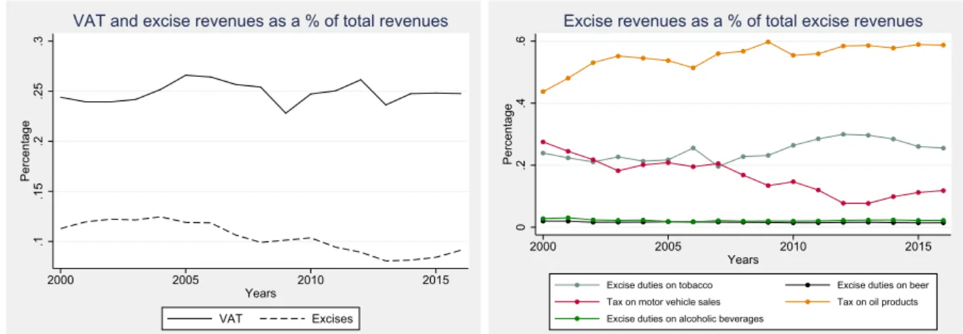
This section presents the main characteristics of the Portuguese indirect tax system. Figure 1 describes how VAT and excise revenues have evolved during the last years in Portugal.

4.1 Value-added taxes

In the European Union (EU), the VAT is a general, broadly based consumption tax on all goods and services. Since it was implemented in France in the late 1940s, it has been applied in several countries.

In Portugal, the VAT law is managed by the Portuguese Tax and Customs Authority (known as Autoridade Tributária e Aduaneira), and it has a special code: (i) Código do Imposto sobre o Valor Acrescentado (CIVA) and (ii) Regime de IVA nas Transaçcões Intracomunitárias (RITI). In Portugal, the VAT was introduced when the country entered the EU in 1986. As member state of the EU, Portugal bases its tax law on regulations drawn up at the European level.5 _{Currently, there are three VAT rates: the standard}

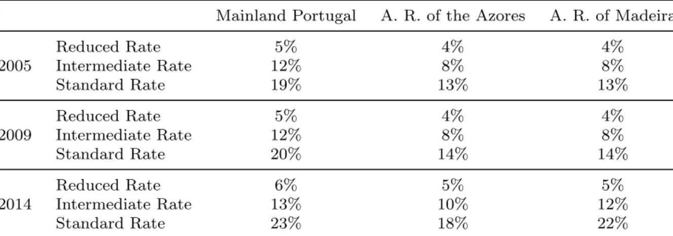
rate of 23%, the intermediate rate of 13% and the reduced rate of 6%. However, the Autonomous Regions of the Azores and Madeira have lower taxes of, respectively, 18% and 22% for the standard one, 4% and 5% for the reduced and 9% and 12% for the intermediate one.

The reduced rate is applied to several commodities like basic food, water supply, spe-cific pharmaceutical products, certain newspapers, periodicals and books, medical equip-ment for disabled, medical services (if not exempt), hotels and similar services, social housing and many agriculture products and services; the intermediate rate is applied to some other food, wine, mineral water, diesel fuel for agriculture, machinery mainly used in agricultural production and admission to cultural events; the standard rate is imposed on most goods and services. Additionally, there are goods and services that are exempt from VAT: housing costs, health expenditures and education expenditures.

5_{Although Portugal is required to comply the VAT code of the EU, the country still sets the level of}

(9)

Table 1 describes the VAT rates that were in force in the years considered in this analysis.

Table 1: VAT Rates in Portugal

Mainland Portugal A. R. of the Azores A. R. of Madeira

Reduced Rate 5% 4% 4% 2005 Intermediate Rate 12% 8% 8% Standard Rate 19% 13% 13% Reduced Rate 5% 4% 4% 2009 Intermediate Rate 12% 8% 8% Standard Rate 20% 14% 14% Reduced Rate 6% 5% 5% 2014 Intermediate Rate 13% 10% 12% Standard Rate 23% 18% 22%

Note: We assume VAT rates before the new VAT schedule of July 2005. Source: Tax and Customs Authority, 2018.

4.2 Excise duties

Excise taxes are levied on certain types of commodities. In Portugal, these commodities can be alcohol and alcoholic beverages, beer, tobacco products, oil and gas. The Por-tuguese tax system covers two types of excise taxes: (i) specific taxes, which impose a fixed amount of euros for each unit of product, regardless of the price charged (e.g. per hectoliter or grams) and (i) ad valorem taxes, that are levied based on the value (price) of the product. Figure 1 reveals the importance of revenues from oil products taxes, which accounted for about 60% of total excise revenues in 2016. Conversely, in the case of com-modities such as beer and alcoholic beverages, this share is not significant (around 5% of total excise revenues).

In Portugal, the tax on alcohol and alcoholic beverages is generally known as imposto sobre o ´alcool e as bebidas alco´olicas (IABA) and it is levied on alcoholic beverages (beer,

Table 2: Tax on alcohol and alcoholic beverages in 2018

Product Limit

Beer Frome 7.75/hl to e 27.24/hl

Wine and other fermented and sparkling beverages e 0

Intermediate products e 70.74/hl

Ethyl alcohol e 1,251.72/hl

Spirit drinks e 1,289.27/hl

(10)

Figure 1: Evolution of indirect tax revenues in Portugal .1 .15 .2 .25 .3 Percentage 2000 2005 2010 2015 Years VAT Excises

VAT and excise revenues as a % of total revenues

0 .2 .4 .6 Percentage 2000 2005 2010 2015 Years

Excise duties on tobacco Excise duties on beer

Tax on motor vehicle sales Tax on oil products

Excise duties on alcoholic beverages

Excise revenues as a % of total excise revenues

Source: Authors’ construction, based on OECD Statistics.

Table 3: Tax on tobacco products in 2018

Product Tax

Cigarettes

• Specific element ise 88.20

(e 16.30 in the Azores and e 58 in Madeira) • Ad valorem element is 17%

(38% in the Azores and 10% in Madeira) Cigars and cigarillos Ad valorem element is 20%

Fine cut tobaccos and other tobaccos • Specific element ise 0.065/g • Ad valorem element is 20% Source: AICEP Portugal Global.

wines, spirit drinks and other fermented beverages) and on ethyl alcohol. The respective tax rates applicable to such commodities are presented in Table 2.

The tax on tobacco products, known as imposto sobre o tabaco (IT), is charged on cigarettes and smoking tobaccos, cigars and cigarillos, and fine cut tobaccos. The current taxes that are applicable to these commodities are described in Table 3.

The tax on oil and energetic products or imposto sobre os produtos petrol´ıferos e energ´eticos (ISP) is charged on the oil and energetic commodities and “any other products that are used as fuel or carburant in any type of non-stationary engine.”

The vehicle tax (known as Imposto sobre Ve´ıculos or ISV) is a “registration tax levied upon the release of vehicles for private consumption.”

(11)

5 Data and Methodology

This section describes the consumption tax microsimulation model adapted from Decoster (2005). First, we describe and discuss the data employed in this work project, the compu-tation of households’ indirect tax liabilities and the output of the microsimulation model. Lastly, we state the underlying assumptions of the model and some of its limitations.

5.1 The Portuguese household budget survey

This work project uses expenditure micro-data from the Household Budget Survey (HBS), more specifically the 2005-2006, 2010-2011 and 2015-2016 waves (being 2015-2016 the latest available one). They include information from, respectively, 10, 403, 9, 489 and 11, 398 households and from 28, 359, 24, 383 and 29, 091 individuals.

The Household Budget Survey is conducted every five years by Statistics Portugal (Instituto Nacional de Estat´ıstica). In Portugal, it is known as Inqu´erito `as Despesas das Fam´ılias (IOF/IDEF) and it provides detailed information on income distribution of households (including disposable income) and the level and structure of their expenditures, as well as their residence accommodation comfort. It also reports their socio-economic and demographic characteristics.

Any economic study on the distribution of income is directly affected by the method that researches use to measure inequality. As explained by Figini (1998), one of the key concerns related to these studies is the evaluation of the direction and variations in inequality when changes in the composition and size of households are allowed. The usual way in the literature to correct for household size is using equivalence scales, which take into account scale economies within the household. In this analysis, we use the OECD-Modified Scale because it is the current standard scale for OECD and Eurostat. The equivalised disposable income is then computed by dividing total household income by the respective equivalence scale.

The collection of information is made through in-person interviews. Expenditure data is collected by survey papers and the detailed description associated with each consump-tion expenditure was collected and analyzed for coding in the framework of the Classifi-cation of Individual Consumption by Purpose (COICOP).6 _{In the 2005-2006, 2010-2011}

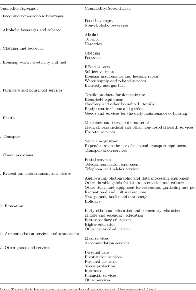
and 2015-2016 waves, expenditure data is based on consumption of 201, 199, 301 goods and services, respectively. Table 7 summarizes the commodity breakdown used for the microsimulation model.

Consumption expenditures are based on four types of periodicity: (i) annually, ap-plicable to goods or services purchased with reduced frequency, such as hospital services

6_{The COICOP is a “classification developed by the United Nations Statistics Division to classify}

and analyze individual consumption expenditures incurred by households, non-profit institutions serving households and general government according to their purpose. It includes categories such as clothing and footwear, housing, water, electricity, and gas and other fuels” (Eurostat definition).

(12)

or car/ insurance purchase; (ii) quarterly, applicable to goods or services purchased sev-eral times a year, but not monthly, such as expenses for clothing, footwear, repair and maintenance of housing; (iii) monthly, applicable to monthly expenses such as leasing, water supply, electricity, and certain types of transport services; (iv) fortnightly, applica-ble to expenditure on goods and services frequently purchased, including food, beverages, tobacco, non-durable household goods, fuels or expenses in restaurants and cafes. After data collection, data on expenditure on goods or services were annualized by applying a multiplicative factor which takes into account the number of periods in the year: 26 in the case of periodicity being fortnightly, 12 in the case of monthly periodicity, and 4 in the case of consumption a which is associated quarterly.

The Horvitz-Thompson estimator is used to estimate households’ weights. All our estimates are corrected for sample weights.7

All forms of monetary income are reported as net-at-source income, which is the income observed in monthly pay slips. Farinha Rodrigues (2007) says that there is evidence showing that most individuals report this type of income. In this work project, we will use net-at-source income as Braz and Correira da Cunha (2009).

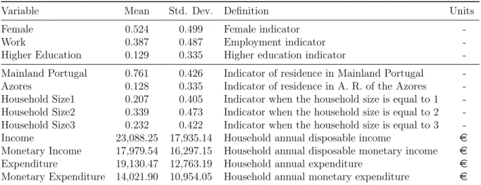
Tables 4, 5 and 6 report descriptive statistics about the HBS.

(13)

Table 4: Descriptive Statistics - HBS 2005/2006

Variable Mean Std. Dev. Definition Units

Female 0.521 0.499 Female indicator

-Work 0.406 0.491 Employment indicator

-Higher Education 0.065 0.247 Higher education indicator

-Mainland Portugal 0.719 0.449 Indicator of residence in Mainland Portugal

-Azores 0.083 0.276 Indicator of residence in A. R. of the Azores

-Household Size1 0.163 0.369 Indicator when the household size is equal to 1

-Income 20,615.31 17,935.14 Household annual disposable income e

Monetary Income 16,458.73 15,976.75 Household annual disposable monetary income e

Expenditure 16,184.00 12,246.99 Household annual expenditure e

Monetary Expenditure 12,027.44 10,477.28 Household annual monetary expenditure e

Source: HBS 2005/2006.

Source: HBS 2010/2011.

(14)

Table 7: Commodity aggregation by COICOP consumption chapters

Commodity Agreggate Commodity, Second Level

1. Food and non-alcoholic beverages

Food beverages

Non-alcoholic beverages 2. Alcoholic beverages and tobacco

Alcohol Tobacco Narcotics 3. Clothing and footwear

Clothing Footwear 4. Housing, water, electricity and fuel

Effective rents Subjective rents

Housing maintenance and housing repair Water supply and related services Eletricity and gas fuel

5. Furniture and household services

Textile products for domestic use Household equipment

Crockery and other household utensils Equipment for home and garden

Goods and services for the daily maintenance of housing 6. Health

Medicines and therapeutic material

Medical, paramedical and other non-hospital health services Hospital services

7. Transport

Vehicle acquisition

Expenditure on the use of personal transport equipment Transportation services

8. Communications

Postal services

Telecommunication equipment Telephone and telefax services 9. Recreation, entertainment and leisure

Audiovisual, photographic and data processing equipment Other durable goods for leisure, recreation and culture Other items and equipment for recreation, gardening and pets Recreational and cultural services

Newspapers, books and stationery Holidays

10. Education

Early childhood education and elementary education Middle and secondary education

Post-secondary education Higher education

Other types of education 11. Accommodation services and restaurants

Meal services

Accommodation services 12. Other goods and services

Personal care Prostitution services Personal use items Social protection Insurance Financial services Other services

(15)

5.2 Households’ indirect tax liabilities

Following the model used by Decoster (2005), we start by matching each category of goods and services in the sample to their corresponding indirect tax rates. It is important to note that all calculations below are made based on the assumption that all goods and services have a fixed price, i.e. producer prices do not vary.

The expression that shows us the relationship between the producer price of good i, bi, and the consumer price, mi, is given by:

mi = (bi+ di+ aibi)(1 + vi) (8)

where di represents the excise per unit, ai the excise expressed as a share of bi and vi

represents the VAT rate. Solving Equation (8) in terms of bi, it follows that:

bi = mi (1 + vi)(1 + ai) − di (1 + ai) (9) The households’ indirect tax liabilities are not only dependent on the tax rates, but also on the consumption pattern, i.e. the relationship between consumption categories (e.g. food, clothing, footwear and health). Denoting xi as the quantity purchased of good

i, the respective tax liability Ti is written as:

Ti = (mi− bi)xi (10)

Since the HBS comprises households’ expenditures, which are dependent on mi, we

need to adjust Equation (3) so that we find an expression in terms of what is observable (HBS does not observe bi). Therefore, by substituting Equation (9) on Equation (10), we

get households’ tax liabilities in terms of observable expenditures and of the parameters of the tax system:

T_ih = vi (1 + vi)(1 + ai) S_ih+ ai 1 + ai S_ih+ di 1 + ai xh_i (11)

where S_ih = mh_ixh_i expresses the expenditure of household h on good i. The first term of Equation (11) represents the VAT component and the second and third elements refer to the excise component. Using Equation (11), the indirect tax liabilities for all households in the HBS were computed.

Tax liabilities were calculated to the twelve commodity aggregates presented in Section 5 (see Table 7), based on the following approach: tax liabilities for each household for commodity aggregate J is given by:

T_Jh =X

j∈J

(16)

Table 8: Evolution of VAT schedule in Mainland Portugal

Date Reduced Rate Intermediate Rate Standard Rate Increased Rate

01/01/1986 0 8 16 30 01/02/1988 0 8 17 30 24/03/1992 - 5 16 30 01/01/1995 - 5 17 -01/07/1996 5 12 17 -05/06/2002 5 12 19 -01/07/2005 5 12 21 -01/07/2008 5 12 20 -01/07/2010 6 13 21 -01/01/2011 6 13 23

-Source: European Commission, 2018.

Afterwards, we get TJ because of the summation of TJh across all households.

5.2.1 Assumptions and limitations Income Data

As it is mentioned in Decoster et al. (2010), there may exist misleading results when considering HBS income data at low income levels. This is justified by the fact that some households have transitorily low incomes, as in the case of self-employed individuals. Con-sequently, and to mitigate this concern, in this analysis we have not considered households that (i) report non-positive income and/or (ii) who have an expenditure-to-income ratio higher or equal to four. In the first case, no household were dropped from the sample. In the second case, in the 2010 and 2015 HBS, 6 and 19 households were eliminated from the sample, respectively.

Consumer Durables

Durables are infrequent purchases and the HBS data provides information on expendi-tures, but also ownership of durable goods. Theoretically, in order to reduce a possible overvaluation (or understatement) of households’ expenditures that were made during (or outside) the period of the survey, the ideal situation would be to distribute the cost of durable goods over its useful life. However, this would not be feasible because we would need accurate information data on length of ownership. However, consumer durables were included in the model, because otherwise we would underestimate households’ consump-tion and tax revenue considerably.

Behavioral Responses

It is a well-known fact that taxes trigger behavioral responses, which may consist in changed quantities, timing of purchase (Drenkard and Henchman, 2016) or location (Ka-plan, 2017). Given that we only have access to a snapshot of consumer expenditure, we cannot model behavioral responses. All our indices are based on a purely mechanical effect

(17)

of the tax, assuming that the consumer demand is inelastic. Therefore, we are likely to achieve less accurate results by not considering behavioral responses, when modeling large changes in VAT rates (where significant responses in consumption behavior are likely). In Table 8, the constant changes that occur in the Portuguese VAT Code are evident. Tax Incidence

This microsimulation model assumes that the final consumer is the one who bears VAT and excise taxes. Nevertheless, in some specific cases, these types of taxes may be less than fully passed out to final consumers, or even more than fully. This assumption is a standard one in this type of studies, used by Decoster et al. (2010), Leahy, Lyons and Tol (2011) or IFS (2011).

Matching of households’ expenditures and corresponding tax rates

There are two commodities that were not included in our analysis: prostitute services and narcotics. It is not possible to match these commodities with a corresponding tax because they are not legal in Portugal. In addition, very few households report any kind of expense in these categories, meaning that their exclusion does not have a significant impact on results.

VAT Exemptions

VAT exemptions are assumed to have zero rates. Excise Taxes

Estimating excise taxes is rather more complex. Excise taxes can be based on quantities purchased or on commodity value. The HBS data includes the quantity of food and drinks consumed by each household. Thus we have access to the amount of alcoholic drinks consumed (beer and spirits), which are used to model the relevant excise taxes.

In the case of tobacco and oil products, there is no data on the quantity purchased. Consequently, in order to simulate these taxes, average prices were used for each excise good to estimate quantities from the HBS data (see Table 9). Here, we assume that both expenditure information and average prices are accurate. Nevertheless, we may have some inaccuracy at the individual level, since we are assuming that households consume higher (lower) quantities than they actually do (some of them consume commodities that have a higher (lower) price than average).

In addiction, we have to consider two additional assumptions: beer and spirits are taxed at different rates because they depend on alcohol content. In our case, we as-sume that all beer has at least 1.2% of alcohol content (and asas-sume this equals 10 to 11 degrees Plato) and for spirits, the Portuguese Code of Special Taxes on Consumption assumes a specific amount of euros per hectoliter consumed (from 1009,36e /hl in 2005 to 1251,72e /hl in 2014); in the case of tobacco products, we use only the ad valorem tax.

(18)

Table 9: Consumer Price Index (CPI)

Alcoholic beverages and tobacco Housing, water, electricity, gas and other fuels

2005 4.7 4.4

2009 3.3 2.1

2014 3.1 2.2

Source: PORDATA.

6 Analysis by Income Deciles

In this section, we analyze the HBS data by income deciles, to better understand the households’ consumption patterns over the years.

Table 10 describes the percentage spent on each tax level and reflects how households’ expenditure composition has changed. It is important to note that these shares include the effect of changes in the tax level.

In 2005, households spent roughly the same on goods taxed at the reduced rate and at the standard rate. As regards to households’ behavior by deciles, the shares are very similar. In 2009, households spent more on goods and services taxed at the standard rate, and this share is higher (lower) for the top (bottom) deciles. In this year, we observe a clear income gradient. In 2014, the goods taxed at reduced rate became the most consumed across all tax levels, although there is an unclear income gradient across deciles. The highest share of reduced rate for poorest households happens in 2014 (almost 50%), showing a greater preference for essential goods and services.

The explanation for this result may be found in the variation of budget shares. Table 11 shows the variation of budget shares for six commodity aggregates, by income decile. There is a clear income gradient across all categories and seems that in 2014, there is a more concentrated expenditure of the poor in essential goods, such as food and housing. In Section 3, the evolution of VAT rates was also analyzed (see Table 1), where we verify the increasing VAT for all tax levels.

Briefly, we observe the following patterns: (i) VAT increased over time for all deciles, (ii) between 2005 and 2009, households consumed less of reduced VAT rate goods (and between 2009 and 2014, the opposite); (iii) in relative terms, poorer households tend to spend more on essential goods, such as food and water, and on services such as education and electricity; (iv) and the households’ expenditure composition has shown significant variations over the years.

(19)

Table 10: Shares spent on each tax level by income decile 2005/2006 Income Deciles Tax Level 0-10 10-20 20-30 30-40 40-50 50-60 60-70 70-80 80-90 90-100 Reduced Rate 0,40 0,39 0,39 0,38 0,38 0,37 0,36 0,36 0,35 0,34 Intermediate Rate 0,09 0,09 0,09 0,09 0,08 0,08 0,09 0,08 0,09 0,08 Standard Rate 0,42 0,43 0,43 0,43 0,43 0,44 0,44 0,44 0,44 0,46 Excise 0,09 0,09 0,09 0,10 0,11 0,11 0,11 0,12 0,12 0,12 2010/2011 Income Deciles Tax Level 0-10 10-20 20-30 30-40 40-50 50-60 60-70 70-80 80-90 90-100 Reduced Rate 0,34 0,33 0,32 0,31 0,29 0,28 0,27 0,27 0,26 0,26 Intermediate Rate 0,13 0,12 0,11 0,11 0,10 0,10 0,09 0,09 0,08 0,07 Standard Rate 0,46 0,48 0,49 0,49 0,51 0,52 0,54 0,55 0,57 0,59 Excise 0,07 0,07 0,08 0,09 0,10 0,10 0,10 0,09 0,09 0,08 2015/2016 Income Deciles Tax Level 0-10 10-20 20-30 30-40 40-50 50-60 60-70 70-80 80-90 90-100 Reduced Rate 0,48 0,47 0,46 0,46 0,45 0,45 0,44 0,43 0,43 0,41 Intermediate Rate 0,10 0,10 0,11 0,11 0,11 0,10 0,12 0,11 0,12 0,12 Standard Rate 0,31 0,31 0,31 0,31 0,32 0,32 0,31 0,33 0,33 0,35 Excise 0,11 0,12 0,12 0,12 0,12 0,13 0,13 0,13 0,12 0,12

(20)

Table 11: Budget shares by income deciles 2005/2006 Income Deciles

Commodity 0-10 10-20 20-30 30-40 40-50 50-60 60-70 70-80 80-90 90-100

Food and non-alcoholic beverages 0,195 0,186 0,179 0,182 0,169 0,164 0,156 0,150 0,138 0,125 Alcoholic beverages and tobacco 0,024 0,020 0,020 0,022 0,020 0,019 0,018 0,014 0,014 0,012 Housing, water, electricity and fuel 0,328 0,331 0,335 0,330 0,319 0,319 0,316 0,308 0,309 0,306 Furniture and household services 0,028 0,030 0,030 0,031 0,031 0,032 0,032 0,034 0,036 0,054

Health 0,084 0,079 0,075 0,068 0,063 0,058 0,058 0,059 0,054 0,052

Education 0,013 0,014 0,015 0,018 0,019 0,021 0,026 0,027 0,031 0,032

2010/2011 Income Deciles

Commodity 0-10 10-20 20-30 30-40 40-50 50-60 60-70 70-80 80-90 90-100

Health 0,074 0,076 0,075 0,069 0,065 0,061 0,067 0,064 0,066 0,062

Education 0,011 0,017 0,010 0,019 0,019 0,020 0,021 0,020 0,023 0,024

2015/2016 Income Deciles

Commodity 0-10 10-20 20-30 30-40 40-50 50-60 60-70 70-80 80-90 90-100

Health 0,078 0,081 0,067 0,073 0,068 0,065 0,070 0,063 0,066 0,065

Education 0,016 0,015 0,015 0,016 0,017 0,017 0,018 0,019 0,019 0,022

Source: Authors’ construction from HSB data.

7 Results

7.1 Kakwani index & Progressivity curves

Figure 2 reveals how the Portuguese indirect fiscal system seems to be regressive. The concentration curve for total indirect taxes is always above the disposable income curve in 2005, 2009 and 2014.

The pattern expressed in Figure 2 can be confirmed by means of the Kakwani index: −0.0846 (in 2005), −0.0572 (in 2009) and −0.1529 (in 2014). The lower (or more negative) the Kakwani index, the less a tax is targeted at the poor households.

This result is in accordance with O’Donoghue et al. (2004), who find that Portugal has a regressive indirect tax system.

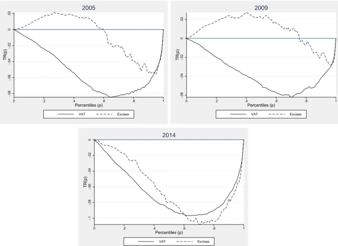
Figure 3 reveals the surprising result that excise taxes are less regressive than VAT (in 2005 and 2009, there are even bottom quintiles where excise taxes are progressive). Even though, this pattern is not evident in the overall results because excise taxes have a lower weight when measuring the overall progressivity of indirect taxes, given the higher share of tax revenues from VAT. This situation is similar to Russia, where Decoster (2005) finds that excise duties are more progressive than VAT.8

(21)

The Kakwani index in 2014 is equal to −0.1529, meaning that this year is the one where the tax system presents a more regressive pattern. Taking into account the analysis of the previous chapter, we perceive that the increase of regressivity in 2014 was accompanied by an increase of the consumption of goods and services with reduced VAT rate.

Figure 2: Concentration and Lorenz curves

0 .2 .4 .6 .8 1 L(p) and C(p) 0 20 40 60 80 100 Percentiles (p)

L(p): Equivalised Disposable Income C(p): Total Taxes

2005 0 .2 .4 .6 .8 1 L(p) and C(p) 0 20 40 60 80 100 Percentiles (p)

2009 0 .2 .4 .6 .8 1 L(p) and C(p) 0 20 40 60 80 100 Percentiles (p)

2014

Source: Authors’ construction, using lorenz, a Stata module to estimate and display Lorenz curves and concentration curves (Jann, 2016).

7.2 The effect of reduced VAT rates as a redistributional tool

In this section, we examine the effectiveness of reduced VAT rates at supporting low-income households.

The existence of goods taxed at reduced rates is usually grounded in socioeconomic motives. This is based on the assumption that some basic goods, such as food, constitute a higher percentage of consumption expenses for low-income earners. Thus, when poli-cymarkers use the reduced VAT rate may be to avoid the regressiveness impact that a standard VAT rate would produce. There are also other cases in which reduced rates are of separate components. These weights are given by the percentage of components in total tax revenue.

(22)

Figure 3: Progressivity curves by indirect tax structure -.08 -.06 -.04 -.02 0 .02 TR(p) 0 .2 .4 .6 .8 1 Percentiles (p) VAT Excises 2005 -.06 -.04 -.02 0 .02 TR(p) 0 .2 .4 .6 .8 1 Percentiles (p) VAT Excises 2009 -.1 -.08 -.06 -.04 -.02 0 TR(p) 0 .2 .4 .6 .8 1 Percentiles (p) VAT Excises 2014

Source: Authors’ construction, using Distributive Analysis Stata Package (DASP).

applied: the case of books or newspapers, in which there is a social concern in promoting these type of goods (or at least, not hinder their consumption).

Reduced VAT rates are expected to have a progressive impact in the sense that they give a higher relative tax reduction to the poor than to the rich. As Table 10 shows, the bottom income deciles have always higher shares of expenditure on goods taxed at reduced rates. However, because richer households consume more in aggregate terms than poorer households, rich households can still be expected to gain more in aggregate terms from a reduced VAT rate (though still less in relative terms). Furthermore, if a reduced rate is provided for goods or services that the rich consume proportionately more of than the poor then that reduced rate will have a regressive impact. In practice, the size of the tax reduction from a reduced VAT rate will depend on the actual consumption patterns of households, which are captured in the HBS data (Martins, 2006).

To investigate the distributional impact of reduced VAT rates, we use the same mi-crosimulation model to simulate the imposition of the standard VAT rate on all items currently subject to reduced or zero VAT rates. By means of the Kakwani index (see

(23)

Table 12: Kakwani index Actual VAT Simulated VAT

2005 - 0.0846 - 0.2764

2009 - 0.0572 - 0.2330

2014 - 0.1529 - 0.3375

Source: Authors’ calculations, using progres, a Stata module for assessing the distributive effects of an income tax (Peichl and van Kerm, 2007).

Table 12) and progressivity curves (see Figure 4), we show that the reduced VAT rates clearly reduce the regressivity of indirect tax system overall, having the desired “progres-sive effect”.

8 Conclusion

In this work project, we have examined the distributional impact of the Portuguese in-direct tax system and shown how the progressivity of Portugal’s inin-direct tax system has evolved, by means of a microsimulation model. A set of different tools for study progres-sivity have been used, such as progresprogres-sivity curves and Kakwani progresprogres-sivity index.

Our findings, using the Household Budget Survey data for the last three waves, show a clear regressive incidence of the Portuguese indirect taxation, and 2014 seems to be the year where the tax system had the highest regressivity pattern. It is also shown that there was a significant change in the composition of expenditures per tax level. Additionally, we investigated the distributional impact of reduced VAT rates and our findings suggest that reduced VAT rates can reduce the regressivity of indirect tax system overall, having the desired “progressive effect” that policymakers desire.

An important contribution of this work project is the analysis of tax progressivity taking into account the two Autonomous Regions of Portugal. It has already been men-tioned that both have slightly different tax systems compared to Mainland Portugal, and considering this fact, we have got more accurate results.

The conclusions drawn from this analysis may encourage policymakers to apply fiscal policies that can generate a higher impact on tax progressivity.

The main limitation of this work project is the quality of the data, given the high possibility of measurement error. Kasprzyk (2005) identifies four sources of measurement error in sample surveys: “the questionnaire, the data-collection mode, the interviewer, and the respondent”.

This analysis could be extended in a number of interesting ways. One way to improve this research would be to use a health survey, in addition to the HBS. Creating an ad-ditional section based on health reports and focusing on excise taxes would allow us to

(24)

Figure 4: Progressivity curves with actual and simulated VAT rates -.2 -.15 -.1 -.05 0 TR(p) 0 .2 .4 .6 .8 1 Percentiles (p)

Actual VAT Rates Simulated VAT Rates

2005 -.2 -.15 -.1 -.05 0 TR(p) 0 .2 .4 .6 .8 1 Percentiles (p)

2009 -.2 -.15 -.1 -.05 0 TR(p) 0 .2 .4 .6 .8 1 Percentiles (p)

2014

Source: Authors’ construction, using Distributive Analysis Stata Package (DASP).

check a possible “under-reporting on the distributional pattern of indirect tax liabilities” (Decoster, 2005). This under-reported consumption of specific commodities generally oc-curs when the respondents assess these commodities as “bads”. Decoster (2005) found out significant differences between these two data sources.

Another way to improve this analysis would be to use the net-gross conversion proposed by Farinha Rodrigues (2007) and implemented by Matos (2018), instead of using net-at-source incomes, and to perform the decomposition of the indirect tax progressivity into vertical, horizontal and reranking effects (see Braz and Correia da Cunha, 2009).

References

[1] Blum, Walter J., and Harry Kalven. “The uneasy case for progressive taxation.” (1954).

[2] Braz, Cl´audia and J. Correia da Cunha. “The Redistributive Effects of VAT in Portugal.” Economic Bulletin (2009): 71-86.

(25)

[3] Caspersen, Erik, and Gilbert Metcalf. “Is a value added tax progressive? Annual versus lifetime incidence measures”. No. w4387. National Bureau of Economic Research, 1993.

[4] Costa Matos, Miguel. How Progressive are Portugal’s Taxes?. Diss. 2018.

[5] Decoster, A. “How progressive are indirect taxes in Russia?”. Economics of Transition, Volume 13 (4) 2005, 705-729.

[6] Decoster, Andr´e, Jason Loughrey, Cathal O’Donoghue, and Dirk Verwerft. “How regressive are indirect taxes? A microsimulation analysis for five European countries.” Journal of Policy analysis and Management 29, no. 2 (2010): 326-350.

[7] Drenkard, Scott, and Joseph Henchman. “Sales Tax Holidays: Politically Expedient but Poor Tax Policy 2016.” Tax Foundation Special Report 233. 2016. Washington, DC.

[8] Figini, Paolo. “Inequality measures, equivalence scales and adjustment for household size and composition.” No. 185. LIS Working Paper Series, 1998.

[9] Formby, John P., Terry G. Seaks, and W. James Smith. “A comparison of two new measures of tax progressivity.” The Economic Journal 91, no. 364 (1981): 1015-1019.

[10] Huesca, Luis, and Abdelkrim Araar. “Progressivity of taxes and transfers: the Mexican case 2012.” (2014).

[11] IFS (2011), “Quantitative analysis of VAT rate structures” in IFS et al., A retrospective evaluation of elements of the EU VAT system, Report prepared for the European Commis-sion.

[12] Jann, Ben. Estimating Lorenz and concentration curves in Stata. University of Bern Social Sciences Working Paper No. 15. (2016).

[13] Jann, Ben. “LORENZ: Stata module to estimate and display Lorenz curves and concen-tration curves.” (2016).

[14] Kakinaka, Makoto and M. Pereira, Rodrigo. “A New Measurement of Tax Progressivity”. (2006).

[15] Kakwani, Nanak C. “Measurement of tax progressivity: an international comparison.” The Economic Journal 87, no. 345 (1977): 71-80.

[16] Kaplan, Jennifer. (2017) “Philadelphia’s Soda Sellers Say Tax Has

Re-duced Sales by as Much as 50%.” Web. Bloomberg. Accessed at

https://www.bloomberg.com/news/articles/2017-02-17/philly-soda-sellers-say-tax-has-reduced-sales-by-as-much-as-50 on 18th December 2018.

[17] Kasprzyk, Daniel. “Measurement error in household surveys: sources and measurement.” Mathematica Policy Research, 2005.

(26)

[18] Leahy, Eimear, Se´an Lyons, and Richard SJ Tol. “The distributional effects of value added tax in Ireland.” The Economic and Social Review 42, no. 2 (2011): 213.

[19] Martins, Ana. Progressivity in the Portuguese personal income tax system. Diss. 2016.

[20] Musgrave, Richard A., and Tun Thin. “Income tax progression, 1929-48.” Journal of po-litical Economy 56, no. 6 (1948): 498-514.

[21] OECD (2018), “Consumption Tax Trends 2018: VAT/GST and Excise Rates, Trends and Policy Issues”, OECD Publishing, Paris.

[22] OECD (2018), “Revenue Statistics 2018”, OECD Publishing, Paris.

[23] OECD/Korea Institute of Public Finance (2014), “The Distributional Effects of Consump-tion Taxes in OECD Countries”, OECD Tax Policy Studies, No. 22, OECD Publishing.

[24] O’donoghue, Cathal, Massimo Baldini, and Daniela Mantovani. “Modelling the redistribu-tive impact of indirect taxes in Europe: an application of EUROMOD”. No. EM7/01. EUROMODWorking Paper, 2004.

[25] Peichl, Andreas, and Philippe Van Kerm. ”PROGRES: Stata module to measure distribu-tive effects of an income tax.” (2007).

[26] Rodrigues, C. F. “Income in EU-SILC-Net/gross conversion techniques for building and using EUSILC databases.” Comparative EU Statistics on Income and Living Conditions: Issues and Challenges (2007): 157-172.

[27] Vickrey, William Spencer. “Agenda for progressive taxation.” Ronald Press Company, 1947.

[28] Wagstaff, Adam, Eddy Van Doorslaer, Hattem van der Burg, Samuel Calonge, Terkel Christiansen, Guido Citoni, Ulf-G. Gerdtham et al. “Redistributive effect, progressivity and differential tax treatment: Personal income taxes in twelve OECD countries.” Journal of Public Economics 72, no. 1 (1999): 73-98.

[29] Web. AICEP Portugal Global. 2018. Accessed at

http://portugalglobal.pt/EN/InvestInPortugal/fiscalsystem/Paginas/OtherTaxes.aspx on 2nd December 2018.

(27)

9 Appendix

Figure 5: Density curves of equivalised disposable incomes

0 .00002 .00004 .00006 .00008 .0001 Density 0 20000 40000 60000

Equivalised Disposable Income

2005 2009 2014

Source: Authors’ construction from HBS data.

Figure 6: Total tax liabilities as a share of total expenditure

0 5 10 15 Density 0 .1 .2 .3 .4

Total Tax Liability/Total Expenditure

2005 2009 2014

(28)

Figure 7: Progressivity curves -.08 -.06 -.04 -.02 0 TR(p) 0 .2 .4 .6 .8 1 Percentiles (p) 2005 -.04 -.03 -.02 -.01 0 TR(p) 0 .2 .4 .6 .8 1 Percentiles (p) 2009 -.1 -.08 -.06 -.04 -.02 0 TR(p) 0 .2 .4 .6 .8 1 Percentiles (p) 2014

(29)

Figure 8: Progressivity curves by NUTS -.1 -.05 0 .05 TR(p) 0 .2 .4 .6 .8 1 Percentiles (p)

Portugal Mainland A. R. Azores A. R. Madeira

2005 -.05 -.04 -.03 -.02 -.01 0 TR(p) 0 .2 .4 .6 .8 1 Percentiles (p)

2009 -.1 -.08 -.06 -.04 -.02 0 TR(p) 0 .2 .4 .6 .8 1 Percentiles (p)

2014