Contagion intra-industry effects of bankruptcies

(1)

Contagion intra-industry

effects of bankruptcies

Filipe Perre da Silva

Dissertation written under the supervision of professor Diana Bonfim.

Dissertation submitted in partial fulfilment of requirements for the MSc in

Finance, at the Universidade Católica Portuguesa, January 2020.

(2)

Contagion intra-industry effects of bankruptcies

Filipe Perre da Silva

Abstract:

This dissertation investigates the effect of bankruptcies on the industry performance, focusing on the bankrupt firm’s competitors. We test whether the market reacts only on the day of the filling to Chapter 7 (as proven in the previous literature) or if the market also reacts on the day of the effective bankruptcy. In industries with a low degree of competition there is a statistically significant decrease in the industry’s returns during a 11 days period (being the 6th_{day, the day}

when the firm is delisted from the stock market), with an average daily return of -0.137%. The same happens for industries with a high degree of competition, with an average daily return of -0.081%. Industry 6000 – “Finance, Insurance and Real Estate” presents the best results to provide evidence for the hypothesis that the market reacts on the announcement and on the effective day of the bankruptcy, with an average excess return for the 3 days (being the 2nd_day,

the day when the firm is delisted from the stock market) of -0.28%.

(3)

Efeito de contágio intraindustrial de falências

Filipe Perre da Silva

Abstrato:

Nesta dissertação é investigado o efeito das falências no desempenho da indústria, com foco nos concorrentes da empresa falida. A hipótese é se o mercado reage apenas no dia do preenchimento do capítulo 7 (conforme provado na literatura anterior) ou se o mercado também reage no dia efetivo da falência. Nas indústrias com baixo grau de concorrência, há uma diminuição estatisticamente significativa dos retornos da indústria durante o período de 11 dias (sendo o 6º dia, o dia em que a empresa é retirada da bolsa), com um retorno médio diário de -0,137%. O mesmo ocorre para indústrias com elevado grau de concorrência, com retorno médio diário de -0,081%. O setor 6000 - “Finanças, Seguros e Imobiliário” apresenta os melhores resultados para evidenciar a hipótese de que o mercado reage ao anúncio e no dia efetivo da falência, com retorno excedente médio nos 3 dias (sendo o 2º dia, o dia em que a empresa é excluída do mercado de ações) de -0,28%.

(4)

Acknowledgments

First, I would like to thank my supervisor professor Diana Bonfim whose guidance was fundamental for the completion of my dissertation.

A special thanks to my friends who helped me a lot during the all process, some from the first grade until the end of my master, some less time, but a huge ‘Thank you!’ for all of you. Also, I would like to thank Católica for providing me the best time I ever had in any school/college. I can say that I enjoyed (almost) every minute that I spent here. I will really miss all the coffees, lunches, dinners, but not the exams! Now, I can proudly say that I belong to Católica’s alumni.

With these, I must thank professor José Faias for coordinating my master program and all the other professors that shared their knowledge with me.

Finally, I want to thank my parents and grandparents that without them none of this would be possible. I hope that by completing my studies I make all of you proud.

(5)

List of Figures

(7)

List of Tables

Table 1: Number of bankruptcies per industry. ... 11

Table 2: Standard Industrial Classification division. ... 13

Table 3: Industry daily reaction to a bankruptcy inside that industry. ... 16

Table 4: 11 and 3-days average industry reaction to a bankruptcy. ... 17

Table 5: Regression's output. ... 18

Table 6: Daily industry reaction to a bankruptcy for each firm. ... 26

Table 7: Summary statistics. ... 30

(8)

List of Abbreviations

AMEX – American Stock Exchange CDS – Credit Default Swap

CRSP - Center for Research on Security Prices ER – Excess Return

Etc – et cetera

EU – European Union i.e. – id est

NASDAQ - National Association of Securities Dealers Automated Quotations NYSE – New York Stock Exchange

SIC Code – Standard Industrial Classification Code US – United States of America

(9)

1. Introduction

It has been proven before that, on average, a bankruptcy announcement has a strong negative effect on the value of the filing firm’s stock (Altman, 1969; Clark and Weinstein, 1983). This decrease on the stock prices is usually linked to the increase in the present value of bankruptcy cost. Yet, the stock price reaction does not reveal if the bankruptcy effects are firm-specific or industry-wide. Bernanke (1983) and Lang and Stulz (1992) claim that a bankruptcy is contagious within an industry. This claim is based on two facts: (i) a bankruptcy announcement reveals negative information about the components of cash-flow that are common to all firms in the industry, and consequently, decreases market’s expectations of the profitability of the industry’s firms; (ii) after a firm’s bankruptcy, suppliers and customers fear that other firms inside the industry will follow the path and so makes them worse off.

Lang and Stulz (1992) found that, on average, the market value of a value-weighted portfolio of the common stock of the bankrupt firm’s competitors decreases 1% at the time of the bankruptcy announcement and this decline is statistically significant. This effect is even higher for highly leveraged industries (debt-to-asset ratio above the sample median): the value of competitors’ equity drops by almost 3% on average. Yet, if the bankruptcy announcement redistributes wealth from the bankrupt firm to their competitors, it can increase the value of the non-bankrupt firms in the industry (Altman, 1984). Lang and Stulz (1992) found that in a low leverage industry, with a high concentration level (using the Herfindahl index of industry concentration as a proxy for the degree of imperfect competition), the value of the bankrupt firm competitors’ equity actually increased by 2.2% on average. On the other hand, industries with high leverage and high degree of competition, the value of competitors’ equity drops to 3.2% on average. The authors provide evidence that a bankruptcy announcement has both a competition and contagion effect on other firms inside an industry.

However, I am interested in studying the effect on the industry performance on the moment the firm is extinguished, meaning I am using the 5 days before and after industry returns when the bankruptcy occurs. With this, I intend to see if there is any effect on the industry returns after a firm extinguish and if yes, to see whether it was caused by contagion, competition, information, counterparty or cascade effect. However, some effects cannot be measured through my regression: information, cascade and counterparty. Information effects as found before by Chakrabarty and Zhang (2012), only intensify the effects, meaning that alone they do not cause a meaningful impact on the returns of an industry. Knowing that cascade effects happen

(10)

whenever a firm’s bankruptcy is followed by another firm’s bankruptcy, caused by the business ties between the two firms, my regression will not be able to capture this effect. Counterparty effect is caused by business ties between firms from different industries and due to this fact, I will not be able to capture this effect on my regression (limited information on the databases used concerning this type of data). If there is no effect on the returns, it means the market had already adjusted at the moment of the filling on Chapter 7: it controls the process of asset liquidation in United States (a trustee is appointed to liquidate nonexempt assets to pay creditors; after the proceeds are exhausted, the remaining debt is discharged).

Banks’ failures will not be covered in this dissertation since there are heavily regulated due to the consequences they can have on the economy of the country where the bankruptcy happened. Moreover, most banks file for Chapter 11 which can also be called rehabilitation bankruptcy. This gives the firm the opportunity to reorganize its debt and to try to reemerge as a healthy organization, meaning the firm will contact its creditors in an attempt to change the terms on loans, such as the interest rate and dollar value of payments. Also, some banks can be acquired by other operating banks while selling their ‘bad’ assets to the government – the so called ‘too big to fail policy’. The government assures the major part of the debt in order to avoid catastrophic consequences to the country’s economy. For instance, in the United States, the Federal Deposit Insurance Corporation closely follows the bank failures: in 2019, four banks failed – City National Bank of New Jersey, Resolute Bank, Louisa Community Bank and The Enloe State Bank. However, other banks assumed the operations of the failed banks whilst the United States government assumed part of the ‘bad’ assets in order to avoid a higher negative impact to the economy. Since the complexity of this type of bankruptcies is extreme, this dissertation will not cover them.

As previously mentioned, I intend to see if there is any effect on the industry returns after a firm is extinguished and, if yes, to see whether it was caused by contagion or competition. These effects are defined as follows.

The contagion effect can be defined as the change in competitors’ value which cannot be attributed to wealth redistribution from the bankrupt firm. If one views a firm as a portfolio of investments that its true value is not known to outside investors, a bankruptcy filing exposes information to outsiders about that value. Knowing that a bankruptcy is costly, the bankrupt firm could avoid this situation by raising funds if the value of its investments was higher. The other firms inside the industry are expected to have investments with cash-flow characteristics very similar to the bankrupt firm. The bankruptcy announcement also carries bad news about these firms since the value of their investments is correlated with the value of the bankrupt

(11)

firm’s investments. For industries with firms with highly similar cash-flow characteristics, it is expected the contagion effect to be more impactful than for other industries, all else being equal. The bankruptcy announcement, in addition to revealing negative information, can decrease the market value of competitors by affecting their dealings with clients, suppliers and regulators. For instance, customers with limited information about individual firms in an industry might reconsider their perception of the creditworthiness of all firms in the industry. Consequently, these firms can experience a fall in demand and a need to advertise their creditworthiness. A simple scenario that leads to a competitive effect is as follows: inside an industry with imperfect competition, meaning each firm faces an imperfectly elastic demand curve, if one assumes that the bankrupt firm suffers an unexpected decrease in demand due to its product becoming less attractive comparing to the competitors’ products, it means that this demand decrease might result from the bankruptcy itself as an indirect bankruptcy cost or from past developments. If the bankruptcy announcement carries information about the demand shift, this information is positive for the other firms inside the industry because they have experienced or can expect an increase in demand.

The other effects that will not be tested are defined as follows.

The counterparty effect will affect the firms who lent money, such as a clients or suppliers account, to the bankrupt firm or were exposed to losses from financial market transactions, such as through CDS.

Tangent with the contagion effect, the information effect, by reveling to the market the real conditions of the industry where a bankruptcy occur, can lead to the loss of trust by customers, regulators, and suppliers and therefore affect the deals other firms intend to do. Once again, it can be costly to advertise their creditworthiness, for instance, and the companies inside the industry will be harmed by the spread of this type of information.

Finally, the cascade effect happens whenever a firm’s bankruptcy is followed by another firm’s bankruptcy, caused by the business ties between the two firms.

Figure 1 describes channels of contagion.

Figure 1: Channels of Contagion Effect

The following figures describes the channels of contagion effect after a bankruptcy which can be divided into five different effects: contagion, information, competition, counterparty and cascade. When a Firm A files for bankruptcy, or defaults, one generally expects negative effects for other firms inside the same industry. Contagion effects reflect negative common shocks to the forecasts of the industry and might lead to further failures in Industry A. However, the

(12)

failure of a firm may help its competitors gain market share. Normally, on the other hand, the net of these two effects is intra-industry contagion. Contagion effects can also arise across industries. Presume that Industry A is a major client of Industry B. The default of Firm A can then reveal negative information concerning sales prospects for firms inside Industry B. Another channel is the direct counterparty effect. Consider that Firm B has made a loan to Firm A. If Firm A defaults, it would cause a direct loss to Firm B, possibly leading to financial distress. This could cause cascading effects to Firm B’s creditors.

The data concerning the bankrupt firms is retrieved from the Center for Research on Security Prices (CRSP), with daily frequency. The sample covers the entire US stock market including NYSE, AMEX & NASDAQ. All the returns are expressed in USD. Moreover, for the scope of my analysis, I obtain the 49 Industry Portfolios from Kenneth R. French Data Library Website, including dividends and daily returns. All the excess returns are measured with respect to the US treasury-bills also sourced from Kenneth R. French Data Library Website. The final sample consists of 152 firms over the time period of January 1990 up to December 2018.

I found that on the day of the effective bankruptcy all industries present a negative return on that day, excluding one industry (“Transportation, Communications, Electric, Gas and Sanitary

Business Conditions Industry A Industry B Firm A files for bankruptcy Industry rivals All firms in Industry B Firm B creditor of Firm A Contagion effect Counterparty effect Contagion/

Competition effect _counterpartyCascading

effect

(13)

service”), and the returns vary between -0.48% on “Services” and -0.05% on “Agriculture, Forestry, Fishing, Mining and Construction”. Despite the fact that on the previous and subsequent days of the bankruptcy, the returns seem to act randomly- confirming the suspicious of the stock market adjusting on the day of the announcement and not on the day of the actual bankruptcy- the day 0 presents a negative, or null in one case, return on every industry.

Also, I checked the 3-day and 11-day performance with the middle day being the day of the effective bankruptcy, i.e. no further presence on the stock market. The results for the 11-day performance were not consistent between each industry, meaning there was no pattern to explore, i.e. the market adjusted the returns on the announcement day. However, apart from two industries that presented positive returns (“Manufacturing”, 0.05% and “Wholesale Trade, Retail Trade”, 0.10%), the 3-day average return presented negative results, such as -0.31% for “Agriculture, Forestry, Fishing, Mining and Construction” and -0.14% for “Finance, Insurance and Real Estate” and “Services”, which may lead to think that the market, despite the adjustment seen on 11-day performance, still might react negatively to the extinguish of a firm. Through the regression, I found that the amount of leverage chosen by the firm will not have impact on the industry performance. This can be explained by the fact that the lenders of the firm are not in the same industry as the bankrupt firm, therefore their competitors will not suffer a higher or lower impact depending on the leverage because they do not have this kind of business ties, except in the case of banks (which were not analyzed in this dissertation). Yet, the ‘Degree of Competition’ matters for the industry performance after a bankruptcy, i.e. it is statistically significant. It reduces the industry returns on the effective day of the bankruptcy in a presence of a low or high degree of competition by -0.137% and -0.081%, respectively. Regarding the industry itself, three reveal a statistically significant negative effect when a bankruptcy occurs inside that industry: 3000 – “Manufacturing”, 4000 – “Transportation, Communications, Electric, Gas and Sanitary service” and 5000 – “Wholesale Trade, Retail Trade”. In the day of an effective bankruptcy, those industries report a return of 0.185%, -0.154% and -0.291%, respectively. The constant of the regression is used as a proxy for the contagion effect. However, the results show inconsistency with the results found by Lang and Stulz (1992): there is no presence of contagion effect on the bankruptcies analyzed. However, this research proved partially the competition effect through the variable ‘Degree of Competition’, as found by the beforementioned authors. This means that, on this research, I was able to prove the negative effect for highly competitive industries in line with Lang and Stulz (1992), with the same happening to industries with a low degree of competition as opposed to the authors.

(14)

As previously stated, the objective of this dissertation is to check if the market also reacts to an extinction of a firm on the effective day of the bankruptcy or if the market (only) reacts on the day of the announcement, as proven by several authors such as Lang and Stulz (1992), paper which I based myself for this investigation. Since the day of the announcement can be unpredictable, therefore one cannot extract a benefit from it. However, if the market also reacts to the extinguish of a firm on the effective day of the bankruptcy (which is known after the firm’s filling), there is a possibility to take an advantage of it and believe that is why my work can be considered as relevant and, hopefully, profitable.

The paper proceeds as follows. In section 2, I expose the previous findings regarding bankruptcy events. I present the data and methodology applied for this event study in section 3. Section 4 covers an extended version of the results and in section 5, I present the concluding remarks of this paper. Afterwards there is a section for the appendix, which includes part of the data I used for this research and another section containing the detailed references of the works mentioned and based for the elaboration of this dissertation.

(15)

2. Literature Review

The announcement of corporate failure normally carries important information regarding the future risk profile and market value of a firm’s shares, such as recovery rate risk (Altman et al., 2005). As found by Clark and Weinstein (1983), a bankruptcy announcement might signal changes in the probabilities of alternative future share values (bankruptcy increases the possibility that the shares will become worthless, for instance). Research to date shows that bankruptcy announcements are normally not complete surprises to the market: the market seizes a solvency deterioration sign into stock returns much before the event of failure. In reality, Aharony et al. (1980) found evidence that shareholders can experience abnormal losses up to a period of 4 to 6 years prior to the announcement of bankruptcy (similar results are reported in Altman and Brenner, 1981; Pettway and Sinkey, 1980; Shick and Sherman, 1980). Moreover, previous literature has reached consensus regarding the effects of a bankruptcy filing on the firm’s competitors: the impact is negative (Helwege and Zhang, 2014). On the case of financial institutions, if they were not extremely ruled, one bankruptcy could lead to a catastrophic event of several bankruptcies followed by the first one (the cascade effect) and consequently a financial crisis. Several authors studied this phenomenon, most focusing on the repercussions which the failure of the Lehman Brothers brought.

a) Events of bankruptcies on financial firms

For financial firms, especially the understanding of the cause of the spillover, is less clear. The most recent financial crisis renewed the interest of what can happen to other firms when a financial institution becomes distressed. The Lehman Brothers, in September 2008, bankruptcy evidenced the negative externalities caused by contagion.

Chakrabarty and Zhang (2012) through this empirical example of a bankruptcy studied the two channels of credit contagion: counterparty risk hypothesis versus information transmission hypothesis. The first one argues that firms with identifiable financial exposure to the bankrupt firm should suffer adverse consequences due to the fundamental business linkage (Davis and Lo, 2001). The latter predicts that the failure of a firm causes investors to update their beliefs, leading to the financial distress of other firms, even when they do not have direct business relationship with the failed firm (Giesecke, 2004; Collin-Dufresne, Goldstein and Helwege, 2010). With the results, the authors were able to find that firms with exposure to Lehman Brothers experienced greater decreases in liquidity and in information asymmetry, higher price impacts of trade, faced higher sell pressure and lower abnormal equity returns than unexposed

(16)

firms – confirming the counterparty contagion hypothesis. Also, the authors claim that the results that pointed for a confirmation of the information transmission hypothesis were mainly driven by counterparty exposure, disregarding the abovementioned hypothesis.

Helwege and Zhang (2014) found that the counterparty contagion affects more larger and riskier firms with complex exposures; yet, for banks which face diversification regulations, the exposure to counterparty contagion is small and does not cause a cascade of failures. Regarding their finding about information contagion, they claim the effects are higher for rivals in the same market and have a more notable impact in the presence of distress rather in bankruptcy. Regarding counterparty contagion, Allen and Gale (2000), Furfine (2003) and Upper and Worms (2004) found that the collapse of one bank causes others to fall in domino-like style due to direct business ties, whether they are clients, vendors who are dependent on the business contracts, other banks or bondholders who provide capital to the financial institution or the ones who become creditors upon a bankruptcy filing. However, many of the financial firms are regulated and benefit from “too big to fail” policy.

Gropp et al. (2003) analyzed bank contagion in a sample of 67 EU banks between 1991 and 2003. The methodology is built upon Bae et al. (2003) and it is related to the extreme value theory, - the behavior of the tail observations for financial market data differs from the other observations. They analyzed the properties of three weekly indicators: (i) the simple first difference of distance to default to measure the absolute shocks, (ii) the log-difference distance to default to measure the percentage shocks and (iii) the abnormal returns for a robustness check. With Monte Carlo simulations, a pattern emerged in the tails of the data and, independently of the measure used, the results are inconsistent with standard multivariate Normal or t-student distributions, suggesting non-linearities. Based on this finding, the authors indicate a non-parametric measure called “net contagious influence”. After controlling for bank size, they were able to precisely measure the contagion between any bank pair, on condition that the probabilities of an idiosyncratic shock hitting the two banks are identical. The results are quite sensible for the majority of the banks and the paper shows that there might be tight links among banks within countries, along with links connecting the major banking systems in Europe. Gropp et al. (2003) claim this paper as a first step towards creating market-based indicators of how vulnerable the banking system may be to contagion as the results may provide a basis to better understand the extent to which European banking system have become interconnected and how banking problems could spread across borders.

(17)

A general study which included all industries, except banks, was done in 1992 by Lang and Stulz. The impact found by the authors differs from the impact caused by financial institutions’ failures.

b) Events of bankruptcy on firms

As previously mentioned, Lang and Stulz (1992) found that, on average, the market value of a value-weighted portfolio of the common stock of the bankrupt firm’s competitors decreases 1% at the time of the bankruptcy announcement and this decline is statistically significant. The data used by the authors covers the entire United States market between January 1970 and December 1989. This effect is even higher for highly leveraged industries (debt-to-asset ratio above the sample median): the value of competitors’ equity drops by almost 3% on average. However, the bankruptcy announcement can increase the value of the non-bankrupt firms in the industry by redistributing wealth from the bankrupt firm to their competitors (Altman, 1984). The authors found that in a low leverage industry, with a high concentration level, the value of competitors’ equity would actually increase by 2.2% on average. On the other hand, industries with high leverage and high degree of competition, the value of competitors’ equity drops to 3.2% on average. Lang and Stulz (1992) deliver evidence that a bankruptcy announcement has both a contagion effect and competition effect on other firms within an industry.

Also, Cheng and McDonald (1996) focused on whether other firms suffer or do not suffer from bankruptcy announcements within the same industry- contagion effect. In this study, the proposition was that the effects of bankruptcy on other firms can be positive, zero or negative. They use the term “ripple effect” instead of contagion effect for negative reactions and competitive effect for positive reactions of nonbankrupt firms to describe the possible bidirectional effects of bankruptcy announcements. By examining the announcement effects of bankruptcy in two industries (the airline and rail-road industries) with very different market structures, the authors found that the airline sample received significant positive abnormal returns (positive ripple) while the railroad sample experienced significant abnormal losses (negative ripple). While, Lang and Stulz (1992) report an insignificant abnormal return for both the airline and railroad industries. The positive stock market reaction in the airline sample does not support the contagion effect hypothesis documented in the literature (Cheng and McDonald, 1996). This study theorizes that market structure is an important factor which may greatly influence the stock market performance of the survivor sample during bankruptcy announcements.

Moreover, Jorion and Zhang (2006) studied the information transfer effect of credit events through the industry, as caught in the stock markets and Credit Default Swaps (CDS), which is

(18)

important to better understand the counterparty effect. They found that negative correlations imply competition effect, while positive correlation across CDS spreads indicate dominant contagion effects. Also, they found strong evidence of dominant contagion effects for Chapter 11 bankruptcies and competition effect for Chapter 7 bankruptcies, confirming, in part, the theories previously discussed. The authors used the example of Enron’s failure: investors were led to reassess their views of the quality of accounting information from other firms. Collin-Dufresne, Goldstein and Helwege (2003) showed that this can lead to a contagion risk premium, previously defined by Giesecke (2004). Most of the times, a contagion effect indicates positive defaults correlations.

(19)

3. Data & Methodology

3.1 Data

The data concerning the bankrupt firms is retrieved from the Center for Research on Security Prices (CRSP), with daily frequency. The sample covers the entire US stock market including NYSE, AMEX & NASDAQ. All the returns are expressed in USD. Moreover, for the scope of my analysis, I obtain the 49 Industry Portfolios from Kenneth R. French Data Library Website, including dividends and daily returns. All the excess returns are measured with respect to the US treasury-bills also sourced from Kenneth R. French Data Library Website.

The initial number of observations was 175 over the time period of January 1990 up to December 2018. However, it was reduced according to different criteria. Firstly, considering that CRSP does not provide data for a bankruptcy, only for delisted firms from the stock market, I also had to extract the delisting code which would provide the information regarding if the firm were delisted because it went private, was bought by another public traded firm or was actually extinguished. Therefore, I only kept the ones that extinguish, meaning the occurrence of a bankruptcy. Then, some firms were too small to cause a meaningful impact on the industry performance after their bankruptcy, therefore firms with less than $10 million in liabilities were excluded. The final sample consists of 152 firms.

It is important to notice the lack of the announcement day on the databases used, therefore the study focused only on the effective day of the bankruptcy.

The following figure explains the match made between the bankrupt firms and the 49 Industry Portfolios.

Table 1: Number of bankruptcies per industry.

The following table describes in (1) the industry, which I further refer as sub-industries, division made by the 49 Industry Portfolios by Kenneth R. French Data Library Website, in (2) the Standard Industrial Classification Code in order to divide each firm into their corresponding industry varying between 1000 and 9000, and in (3) the number of bankruptcies per sub-industry.

This table includes all the bankruptcies in the United States of America between January 1990 and December 2018, excluding firms which were too small to cause a meaningful impact on the industry performance, i.e. liabilities under $10 million. The number of bankruptcies is 152. *Banking industry only includes bankruptcies on the following sub-industries: Finance lessors and Financial services.

(20)

Industry

(1) SIC Code (2) # of bankruptcies (3)

Precious metals 1040 1

Petroleum and Natural Gas 1310 1

Construction 1730 2

Beer and Liquor 2080 1

Textiles 2250 2

Printing and publishing 2730 4

Chemicals 2830 5

Rubber and Plastic Products 3070 1

Apparel 3144 1

Steel Works etc 3312 1

Construction Materials 3440 4

Machinery 3560 2

Computers 3570 6

Electrical Equipment 3600 12

Automobiles and Trucks 3710 2

Aircraft 3720 1

Shipbuilding & Railroad Equipment 3730 1 Measuring and Control Equipment 3820 2

Medical Equipment 3851 1 Consumers Goods 3860 2 Transportation 4000 3 Communication 4840 2 Utilities 4910 2 Sanitary services 4950 3

Steam, air conditioning supplies 4960 1

Wholesale 5000 4 Retail 5620 14 Banking* 6020 15 Trading 6220 9 Insurance 6310 3 Real Estate 6550 3

Restaurants, Hotels and Motels 7010 1

Personal Services 7299 4

Business Services 7310 28

Entertainment 7810 5

Healthcare 8070 3

(21)

Following the data cleaning, each firm had a unique day of bankruptcy. With the 49 Industry Portfolios, I was able to check the previous and after 5 days performance regarding the day of the bankruptcy, by comparing the Standard Industrial Classification (SIC code) to the portfolios provided by Kenneth R. French. Also, I used the 49 Industry Portfolios to test if the returns on the previous and after 5 days on the moment of a bankruptcy were significant or not.

Afterwards, in order to compute a regression to see where the effects are originated, further on deepened, I extracted the current assets and liabilities, total assets and liabilities, debt and cash from Compustat and the returns from CRSP, after merging the two databases through the firms’ Permno (a unique permanent company identification number assigned by CRSP to all companies with issues on a CRSP File) and Cusip (a number which identifies most financial instruments, including: stocks of all registered U.S. and Canadian companies, commercial paper, and U.S. government and municipal bonds. Stands for the Committee on Uniform Securities Identification Procedures).

3.2 Methodology

After obtaining the values for each bankrupt firm, I organized them by industry using the Standard Industrial Classification Code (SIC code) and afterwards I simply averaged the returns for each day within each industry, obtaining this way the average daily return for the time span in analysis: the previous and after 5 days of an effective bankruptcy.

The following figure describes the industry division made.

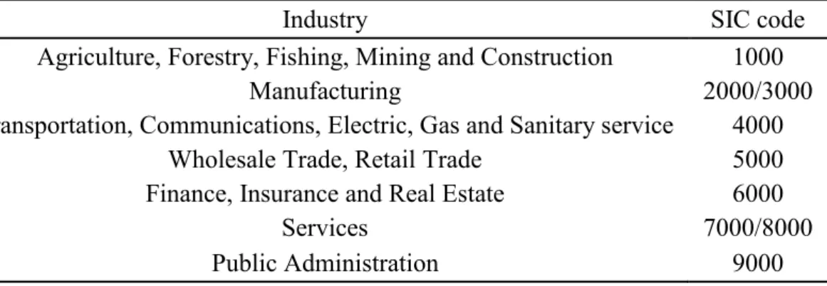
Table 2: Standard Industrial Classification division.

The following table demonstrates the 49 Industry Portfolios by Kenneth R. French Data Library Website comprised into the Standard Industrial Classification.

Industry SIC code

Agriculture, Forestry, Fishing, Mining and Construction 1000

Manufacturing 2000/3000

Transportation, Communications, Electric, Gas and Sanitary service 4000

Wholesale Trade, Retail Trade 5000

Finance, Insurance and Real Estate 6000

Services 7000/8000

(22)

With these values, I was able to see if the effect was negative or positive per day per industry. Then, I averaged the daily values, obtaining the 11-day excess return, being the 6th_{day, the}

effective day of the bankruptcy. Also, I was interested in checking the effect for a shorter time span: the 3-day average return. Therefore, I used the 2nd_{day as the effective day of the}

bankruptcy.

To check whether the returns are statistically significant or not on the period of a bankruptcy, I compared to a non-event industry performance, using the 49 Industry Portfolio. Two methods were used for this check: (i) the average return of the industry on the year of the bankruptcy, ignoring the if there were more bankruptcies on that year and (ii) five random samples of 11 days, excluding the previous and after 5 days of a bankruptcy. However, the first method could capture other significant events and, consequently, would biased the returns of the industry on that year; consequently, the five random samples of 11 days method prevail over the average return of the industry on the year of the bankruptcy. However, both methods matched most the results and the notable differences were on the statistically significance at 1, 5 or 10%, which once again the second method prevailed.

After this, I am able to extract the effects on the returns of the industry after a bankruptcy and to discuss whether the effect is caused by contagion or competition with a regression fitted for this event study.

As mentioned before, some effects cannot be measured through my regression: information, cascade and counterparty. Information effects as found before by Chakrabarty and Zhang (2012), only intensify the effects, meaning that alone they do not cause a meaningful impact on the returns of an industry. Knowing that cascade effects happen whenever a firm’s bankruptcy is followed by another firm’s bankruptcy, caused by the business ties between the two firms, my regression will not be able to capture this effect. Counterparty effect is caused by business ties between firms from different industries and due to this fact, I will not be able to capture this effect on my regression (limited information on the databases used concerning this type of data).

Competition effects can be measured through the coefficient of the dummy variable ‘Degree of Competition’, which was divided into low, medium and high. To determine whether the degree of competition in a specific industry is low, medium or high, I used the data from United States Census Bureau where it is mentioned the concentration of sales and revenues for each industry and therefore, I used it as a proxy (Carlton and Perloff, 1990; Cowling and Waterson, 1976) for the competition inside each industry and then divided into the three categories beforementioned. Since contagion effects can be defined as the change in competitors’ value which cannot be

(23)

attributed to wealth redistribution from the bankrupt firm, this effect will be measured by the regression’s constant, following Lang and Stulz (1992) method. Also, for the regression I included the following variables: ‘Current Ratio’ to check the ability of a firm to pay its short-term obligation; ‘Leverage Ratio’, which is divided into low, medium and high, as a measurement for how much capital comes in the form of debt; an ‘Industry Dummy’ to understand the specific behavior of each industry; ‘Cash over Debt’ to determine whether the company can pay all of its debts if they were due immediately and ‘Assets Over Liabilities’ to see the coverage of a firm’s assets to its obligations were also included on the regression. For the variables ‘Current Ratio’, ‘Cash over Debt’ and ‘Assets over Liabilities’, I expect the higher they are, the higher will be the returns generated through these variables. Concerning the ‘Leverage Ratio’, the lower it is the better for the influence on the returns due to the fact that these firms are a few days from bankruptcy and less debt they have the easier for them to pay to their creditors and therefore, will be a lower leakage of negative information about the firm’s and industry common cash-flow, meaning a less negative impact for the returns of the other non-bankrupt firms. Regarding the ‘Degree of Competition’ it is expected that in a very competitive environment, the old sales of the bankrupt firm will quickly be transferred for another firm in the industry and so the effect should be null; however, if the competition inside an industry is low, it is possible that a bankruptcy will negatively influence the returns, which may be caused by the lost in trust from the clients or investors. In the presence of a contagion effect, the repercussions on the returns are expected to be negative, therefore the coefficient of the regression’s constant is expected to be negative as well. However, the coefficient should not be positive, the maximum statistically significant coefficient which this variable can reach should be 0. Since the contagion effect can be defined as the change in competitors’ value which cannot be attributed to wealth redistribution from the bankrupt firm, it would not be theoretical coherent to have a positive coefficient for the regression’s constant. For the ‘Industry Dummies’ the effect should be coherent with the ‘Degree of Competition’ for that specific industry, meaning if the competition is high in a given industry, the coefficient of the dummy variable should also be null; if it is low, the dummy’s coefficient should be negative.

Finally, the following regression sums up the methodology.

𝑅𝑒𝑡𝑢𝑟𝑛𝑠 𝑖 = 𝐶𝑜𝑛𝑠𝑡𝑎𝑛𝑡 𝑖 + 𝛽1 𝐶𝑢𝑟𝑟𝑒𝑛𝑡 𝑅𝑎𝑡𝑖𝑜 𝑖 + 𝛽2 𝐿𝑒𝑣𝑒𝑟𝑎𝑔𝑒 𝑅𝑎𝑡𝑖𝑜 𝑖 + 𝐷1 𝐿𝑒𝑣𝑒𝑟𝑎𝑔𝑒 𝑅𝑎𝑡𝑖𝑜 (𝐿𝑜𝑤 𝑜𝑟 𝐻𝑖𝑔ℎ) 𝑖 + 𝐷2 𝐼𝑛𝑑𝑢𝑠𝑡𝑟𝑦 𝑖

+ 𝐷3 𝐷𝑒𝑔𝑟𝑒𝑒 𝑜𝑓 𝐶𝑜𝑚𝑝𝑒𝑡𝑖𝑡𝑖𝑜𝑛 (𝐿𝑜𝑤 𝑜𝑟 𝐻𝑖𝑔ℎ) 𝑖 + 𝛽3 𝐶𝑎𝑠ℎ 𝑂𝑣𝑒𝑟 𝐷𝑒𝑏𝑡 𝑖 + 𝛽4 𝐴𝑠𝑠𝑒𝑡𝑠 𝑂𝑣𝑒𝑟 𝐿𝑖𝑎𝑏𝑖𝑙𝑖𝑡𝑖𝑒𝑠 𝑖 + 𝜀 𝑖

(24)

4. Results

4.1 Abnormal returns for each industry in the sample

First of all, after combining each firm into an industry, I obtained the 11-days daily returns for each industry. The following table presents the returns obtained.

Table 3: Industry daily reaction to a bankruptcy inside that industry.

This table includes all the bankruptcies in the United States of America between January 1990 and December 2018, excluding firms which were too small to cause a meaningful impact on the industry performance, i.e. liabilities under $10 million. The number of bankruptcies is 152. After obtaining the values for each bankrupt firm, I organized them by industry using the Standard Industrial Classification Code and afterwards I simply averaged the returns for each day within each industry, obtaining this way the average daily return for the time span in analysis: the previous and after 5 days of an effective bankruptcy. Excess returns are expressed in percentage. Statistical significance of the returns is represented as follows: *** p<0.01, ** p<0.05, * p<0.1, where ‘p’ stands for p-value.

Day relative to bankruptcy 1000 2000 3000 4000 5000 6000 7000 8000 -5 -0.05 0.23 0.23 0.26 -0.34* 0.25 0.08 0.21 -4 -0.27* -0.15* -0.24 0.34 0.32 0.09 -0.20** 0.65* -3 0.59 0.06 -0.34 0.30 0.22 0.27 0.24 0.37 -2 0.81* 0.05 0.32 0.00 -0.22 -0.09 0.10 0.23 -1 0.12 0.51 -0.13* -0.43* 0.26 0.08 -0.08 0.13 0 -0.05 -0.32* -0.36* 0.00 -0.07 -0.17* -0.48*** -0.08 1 -0.98*** -0.04 0.22 0.35 0.11 -0.33** 0.14 -0.07 2 0.45 0.14 0.02 0.03 -0.10 -0.36** 0.34 -0.34 3 0.08 -0.20 -0.20 -0.27* 0.00 0.12 0.09 -0.60* 4 -0.51** 0.35 0.05 0.28 -0.18 0.19 -0.12 -1.16*** 5 0.03 0.10 0.32 0.36* -0.16 0.20 0.30 0.20

As one can see from the table above, on the day of the effective bankruptcy all industries present a negative return on that day, excluding “Transportation, Communications, Electric, Gas and Sanitary service” with 0% on that day, which vary from -0.48% (statistically significant at 1%) on “Services” to -0.05% on “Agriculture, Forestry, Fishing, Mining and Construction”. However, an interesting finding with respect to industry 6000 – “Finance, Insurance and Real Estate” is that the day of the effective bankruptcy and the 2 following days present a return of -0.17%, -0.33% and -0.36%, respectively. It is important to notice that the day 0 is statistically

(25)

significant at 10%, while the two following days are at 1%. This implies an average return for the 3 days of -0.28%.

Despite the fact that on the previous and after days of the bankruptcy, the returns seem to act randomly, confirming the suspicious of the stock market adjusting on the day of the announcement and not on the day of the actual bankruptcy, the day 0 presents a negative, or null in one case, return which I will exploit with the following methodology.

Subsequently, I averaged the daily returns per industry to check the 11-day performance after a bankruptcy. Since the values were not consistent between each other, meaning some were positive some were negative (no arising opportunities from this fact), varying between -0.04% (the only statistically significant return at 10%) on “Services” and 0.11% on “Transportation, Communications, Electric, Gas and Sanitary service”, I shortened the time span to 3 days (one day before and one day after the bankruptcy) and interesting values showed up.

Excluding two industries that present positive returns (“Manufacturing”, 0.05% and “Wholesale Trade, Retail Trade”, 0.10%), the 3-day average return present negative results, such as -0.31% for “Agriculture, Forestry, Fishing, Mining and Construction”, -0.09% for “Manufacturing” and -0.14% for “Finance, Insurance and Real Estate” and “Services”, all statistically significant.

To check whether the returns are statistically significant or not on the period of a bankruptcy, I compared to a non-event industry performance, using the 49 Industry Portfolio: the average of five random samples of 11 days, excluding the previous and after 5 days of a bankruptcy, compared to the excess returns obtained from an actual bankruptcy.

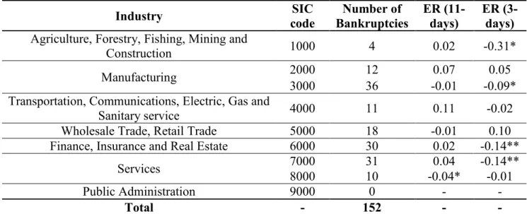
The following table presents the Excess Returns (ER) and the number of bankruptcies for each industry. Statistical significance of the returns is represented as follows: *** p<0.01, ** p<0.05, * p<0.1, where ‘p’ stands for p-value.

Table 4: 11 and 3-days average industry reaction to a bankruptcy.

The following table presents the 11 and 3-days average industry excess returns to a bankruptcy. I averaged the daily values previously obtained in Table 3, obtaining the 11-day excess return, being the 6th_{day, the effective day of the bankruptcy. Also, I was interested in checking the}

effect for a shorter time span: the 3-day average return. Therefore, I used the 2nd_{day as the}

effective day of the bankruptcy.

Excess returns are expressed in percentage. Statistical significance of the returns is represented as follows: *** p<0.01, ** p<0.05, * p<0.1, where ‘p’ stands for p-value.

(26)

Industry _codeSIC _BankruptciesNumber of ER (11-_days) ER (3-_days)

Agriculture, Forestry, Fishing, Mining and

Construction 1000 4 0.02 -0.31*

Manufacturing 2000 12 0.07 0.05

3000 36 -0.01 -0.09*

Transportation, Communications, Electric, Gas and

Sanitary service 4000 11 0.11 -0.02

Wholesale Trade, Retail Trade 5000 18 -0.01 0.10

Finance, Insurance and Real Estate 6000 30 0.02 -0.14**

Services 7000 31 0.04 -0.14**

8000 10 -0.04* -0.01

Public Administration 9000 0 - -

Total - 152 - -

Unfortunately, there was no other combination of days that would provide better results than the Excess Returns 3-days average, i.e. other combinations, such as the 5-day average, would provide positive or null returns and not statistically significant.

4.2 Regression

As previously mentioned, my multivariate analysis is based on the following regression: 𝑅𝑒𝑡𝑢𝑟𝑛𝑠 𝑖 = 𝐶𝑜𝑛𝑠𝑡𝑎𝑛𝑡 𝑖 + 𝛽1 𝐶𝑢𝑟𝑟𝑒𝑛𝑡 𝑅𝑎𝑡𝑖𝑜 𝑖 + 𝛽2 𝐿𝑒𝑣𝑒𝑟𝑎𝑔𝑒 𝑅𝑎𝑡𝑖𝑜 𝑖

+ 𝐷1 𝐿𝑒𝑣𝑒𝑟𝑎𝑔𝑒 𝑅𝑎𝑡𝑖𝑜 (𝐿𝑜𝑤 𝑜𝑟 𝐻𝑖𝑔ℎ) 𝑖 + 𝐷2 𝐼𝑛𝑑𝑢𝑠𝑡𝑟𝑦 𝑖

+ 𝐷3 𝐷𝑒𝑔𝑟𝑒𝑒 𝑜𝑓 𝐶𝑜𝑚𝑝𝑒𝑡𝑖𝑡𝑖𝑜𝑛 (𝐿𝑜𝑤 𝑜𝑟 𝐻𝑖𝑔ℎ) 𝑖 + 𝛽3 𝐶𝑎𝑠ℎ 𝑂𝑣𝑒𝑟 𝐷𝑒𝑏𝑡 𝑖 + 𝛽4 𝐴𝑠𝑠𝑒𝑡𝑠 𝑂𝑣𝑒𝑟 𝐿𝑖𝑎𝑏𝑖𝑙𝑖𝑡𝑖𝑒𝑠 𝑖 + 𝜀 𝑖

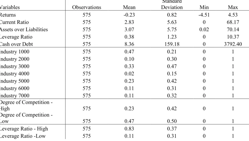
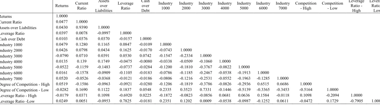
The output of the regression is expressed on the following figure and it was extracted from Stata. Robust standard errors are represented in parentheses and the statistical significance of the coefficient of the variables is represented as follows: *** p<0.01, ** p<0.05, * p<0.1, where ‘p’ stands for p-value. Also, the summary statistics and correlation matrix of these variables can be found on the appendix.

Table 5: Regression's output.

This table includes all the bankruptcies in the United States of America between January 1990 and December 2018, excluding firms which were too small to cause a meaningful impact on the industry performance, i.e. liabilities under $10 million. The number of bankruptcies is 152. The number of observations was 575 with an average of 4 observations per company, i.e. on average every bankrupt firm have their last 4 quarterly trading days present in the regression to

(27)

capture the characteristics which made the firm go bankrupt. Statistical significance is represented as follows: *** p<0.01, ** p<0.05, * p<0.1, where ‘p’ stands for p-value.

Variables Returns

Current Ratio 0.014

(0.012)

Assets over Liabilities -0.008

(0.011)

Leverage Ratio 0.046

(0.057)

Cash over Debt 0.000**

(0.000) Industry 1000 0.098 (0.097) Industry 2000 0.069 (0.131) Industry 3000 -0.185* (0.100) Industry 4000 -0.154*** (0.027) Industry 5000 -0.291*** (0.052) Industry 6000 -0.067 (0.110) Industry 7000 -0.005 (0.014)

Degree of Competition = High -0.081*

(0.047)

Degree of Competition = Low -0.137***

(0.042)

Leverage Ratio Dummy = Low -0.042

(0.105)

Leverage Ratio = High -0.164

(0.350)

Constant 0.010

(0.104)

Number of Observations 575

R-squared 0.021

The number of observations was 575, for the 152 companies with an average of 4 observations per company, i.e. on average every bankrupt firm have their last 4 quarterly trading days present in the regression to capture the characteristics which made the firm go bankrupt.

(28)

Some variables are not statistically nor economically significant. Taking the ‘Leverage Ratio’ into consideration, independent of the amount of debt the firm choses to have, it will not affect the market returns after the bankruptcy. This can be explained by the fact that the lenders of the firm are not in the same industry as the bankrupt firm, therefore their competitors will not suffer a higher or lower impact depending on the leverage because they do not have this kind of business ties, except in the case of banks. This can also be confirmed by the statistically significant coefficient of the ratio ‘Cash over Debt’: it is -0.00023. It matters minimally for the other firms inside that industry if the firm could pay its debts with their available cash or not, since it will almost not affect their performance when a bankruptcy occurs. Also, the ‘Current Ratio’ and the ‘Assets over Liabilities’ do not have an impact on the industry performance. Yet, the ‘Degree of Competition’ matters for the industry performance after a bankruptcy, i.e. it is statistically significant. It reduces the industry returns on the effective day of the bankruptcy in a presence of a low or high ‘Degree of Competition’ by -0.137% and -0.081%, respectively. This finding supports partially the competition effect through the variable ‘Degree of Competition’, i.e., on this research, I was able to prove the negative effect for highly competitive industries in line with Lang and Stulz (1992), with the same happening to industries with a low degree of competition as opposed to the authors.

Regarding the industry itself, three industries reveal a statistically significant negative effect when a bankruptcy occurs inside that industry: 3000 – “Manufacturing”, 4000 – “Transportation, Communications, Electric, Gas and Sanitary service” and 5000 – “Wholesale Trade, Retail Trade”. In the day of an effective bankruptcy, those industries report a return of -0.185%, -0.154% and -0.291%, respectively. These findings go accordingly with the results presented by Lang and Stulz (1992) regarding “the abnormal returns for each industry in the sample” study.

The constant of the regression is used as a proxy for the contagion effect. However, the results show inconsistency with the results found by Lang and Stulz (1992): there is no presence of contagion effect on the bankruptcies analyzed. Since the contagion effect can be defined as the change in competitors’ value which cannot be attributed to wealth redistribution from the bankrupt firm, one can state that a positive statistically significant coefficient would not be coherent with the theory supporting this effect. Thus, a null value is in line with the theory, however does not support the findings of Lang and Stulz (1992).

(29)

4.3 Limitations and further research

The access to some databases, which had the day of the announcement and the day of the effective bankruptcy (such as bankruptcydata.com), were paid and since they did not provide me with the information I needed in order to have a more complete analysis regarding the effects on the returns on both days, I would propose for future studies the beforementioned analysis. It is important to understand if the contagion effect proved by Lang and Stulz (1992) between 1970 and 1989 still stands nowadays and if this is an isolated case in the United States or if this also applies to other regions, especially Europe, since Frino, Jones and Wong (2007) were not able to prove the announcement effect for Australia.

Moreover, some effects such as counterparty and cascade were not analyzed in this dissertation due to the lack of information on the databases used (CRSP and Compustat).

Another limitation was the fact that there are not studies performed only on the effective day of the bankruptcy. The previous literature focused on the day of the announcement and on the effects to the market. I consider that an isolated analysis of this event would be relevant, since the day of the filling to Chapter 7 is not publicly known and the effective the firm stops trading on the stock market is, and one can take advantage of this fact.

Also, as banks’ failures are not covered in this dissertation since there are heavily regulated due to the consequences they can have on the economy of the country where the bankruptcy happened, it would be interesting to see the effect inside the industry (where it is included other financial institutions, insurance companies and real estate firms) and on other industries with and without business ties to the failed bank, when controlled for the macroeconomic consequences in order to extrapolate the contagion and counterparty effect.

(30)

5. Concluding Remarks

This paper provides evidence that an effective bankruptcy has a competitive effect, negative to the returns, on other firms in the same industry independently of having a low or high degree of competition inside that industry (using the Herfindahl index as a proxy for the degree of competition within an industry). However, the results could not support the contagion effect on the effective day of the bankruptcy.

The competitive effect reduces the industry returns on the effective day of the bankruptcy in a presence of a low or high ‘Degree of Competition’ by -0.137% and -0.081%, respectively, both statistically significant. I was able to prove the negative effect for highly competitive industries in line with Lang and Stulz (1992), with the same happening to industries with a low degree of competition as opposed to the authors.

The constant of the regression is used as a proxy for the contagion effect. However, the results show inconsistency with the results found by Lang and Stulz (1992): there is no presence of contagion effect on the bankruptcies analyzed. Since the contagion effect can be defined as the change in competitors’ value which cannot be attributed to wealth redistribution from the bankrupt firm, one can state that a positive statistically significant coefficient would not be coherent with the theory supporting this effect. Thus, a null value, as the one found on this research, is in line with the theory, however does not support the findings of Lang and Stulz (1992).

I found that the leverage ratio, independent of the amount of debt the firm choses to have, will not affect the market returns after the bankruptcy. This can be explained by the fact that the lenders of the firm are not in the same industry as the bankrupt firm, therefore their competitors will not suffer a higher or lower impact depending on the leverage because they do not have this kind of business ties. This can also be confirmed by the statistically significant coefficient of the ratio ‘Cash over Debt’: it is -0.00023. It matters minimally for the other firms inside that industry if the firm could pay its debts with their available cash or not, since it will almost not affect their performance when a bankruptcy occurs. Also, the ‘Current Ratio’ and the ‘Assets over Liabilities’ do not have an impact on the industry performance.

Regarding the industry itself, three reveal a statistically significant negative effect when a bankruptcy occurs inside that industry: 3000 – “Manufacturing”, 4000 – “Transportation, Communications, Electric, Gas and Sanitary service” and 5000 – “Wholesale Trade, Retail Trade”. In the day of an effective bankruptcy, those industries report a return of 0.185%,

(31)

-0.154% and -0.291%, respectively, all statistically significant. These findings go accordingly with the results presented by Lang and Stulz (1992) regarding “the abnormal returns for each industry in the sample” study.

On the day of the effective bankruptcy all industries present a negative return on that day, excluding “Transportation, Communications, Electric, Gas and Sanitary service” with 0% on that day, which vary from -0.48% (statistically significant at 1%) on “Services” to -0.05% on “Agriculture, Forestry, Fishing, Mining and Construction”. However, an interesting finding with respect to industry 6000 – “Finance, Insurance and Real Estate” is that the day of the effective bankruptcy and the 2 following days present a return of -0.17%, -0.33% and -0.36%, respectively. It is important to notice that the day 0 is statistically significant at 10%, while the two following days are at 1%. This implies an average excess return for the 3 days of -0.28%. I performed a 3-day analysis (one day before and one day after the bankruptcy) and, excluding two industries which presented positive returns (“Manufacturing”, 0.05% and “Wholesale Trade, Retail Trade”, 0.10%), the 3-day average return present negative results, such as -0.31% for “Agriculture, Forestry, Fishing, Mining and Construction”, -0.09% for “Manufacturing” and -0.14% for “Finance, Insurance and Real Estate” and “Services”, all statistically significant. The objective of this dissertation is to check if the market also reacts to an extinction of a firm on the effective day of the bankruptcy or if the market (only) reacts on the day of the announcement, as proven by several authors such as Lang and Stulz (1992). Since the day of the announcement can be unpredictable, therefore one cannot extract a benefit from it. However, if the market also reacts to the extinguish of a firm on the effective day of the bankruptcy (which is known after the firm’s filling), there is a possibility to take advantage of it. As one can see from the above results, it is possible to do so for some specific industries and days. The most interesting result is for industry 6000 – “Finance, Insurance and Real Estate” which has average excess return for the 3 days of -0.28%, which provides evidence to the hypothesis that the market reacts on the announcement and on the effective day of the bankruptcy and an investment strategy based on this preposition can lead into a profitable portfolio.

(32)

6. References

Allen, F. and Gale, D., 2000. Financial contagion. Journal of political economy, 108(1), pp.1-33.

Bae, K.H., Karolyi, G.A. and Stulz, R.M., 2003. A new approach to measuring financial contagion. The Review of Financial Studies, 16(3), pp.717-763.

Chakrabarty, B. and Zhang, G., 2012. Credit contagion channels: Market microstructure evidence from Lehman Brothers’ bankruptcy. Financial Management, 41(2), pp.320-343.

Cheng, L.T. and McDonald, J.E., 1996. Industry structure and ripple effects of bankruptcy announcements. Financial Review, 31(4), pp.783-807.

Collin-Dufresne, P., Goldstein, R. and Helwege, J., 2003. Are jumps in corporate bond yields priced? Modeling contagion via the updating of beliefs. University of California Berkeley Working Paper.

Cowling, K. and Waterson, M., 1976. Price-cost margins and market structure. Economica, 43(171), pp.267-274.

Davis, M. and Lo, V., 2001. Modelling default correlation in bond portfolios. Mastering risk, 2(1), pp.141-151.

Dean, T.J. and Brown, R.L., 1995. Pollution regulation as a barrier to new firm entry: Initial evidence and implications for future research. Academy of Management Journal, 38(1), pp.288-303.

Frino, A., Jones, S. and Wong, J.B., 2007. Market behaviour around bankruptcy announcements: evidence from the Australian Stock Exchange. Accounting & Finance, 47(4), pp.713-730.

Furfine, C.H., 2003. Interbank exposures: Quantifying the risk of contagion. Journal of money,

(33)

Giesecke, K., 2004. Correlated default with incomplete information. Journal of Banking & Finance, 28(7), pp.1521-1545.

Gropp, R. and Moerman, G., 2004. Measurement of contagion in banks’ equity prices. Journal

of International Money and Finance, 23(3), pp.405-459.

Helwege, J. and Zhang, G., 2015. Financial firm bankruptcy and contagion. Review of

Finance, 20(4), pp.1321-1362.

Jorion, P. and Zhang, G., 2007. Good and bad credit contagion: Evidence from credit default swaps. Journal of Financial Economics, 84(3), pp.860-883.

Jorion, P. and Zhang, G., 2009. Credit contagion from counterparty risk. The Journal of

Finance, 64(5), pp.2053-2087.

Lang, L.H. and Stulz, R., 1992. Contagion and competitive intra-industry effects of bankruptcy announcements: An empirical analysis. Journal of financial economics, 32(1), pp.45-60.

Upper, C. and Worms, A., 2004. Estimating bilateral exposures in the German interbank market: Is there a danger of contagion?. European economic review, 48(4), pp.827-849.

(34)

7. Appendices

Table 6: Daily industry reaction to a bankruptcy for each firm.

The returns are expressed in percentage. This table includes all the bankruptcies in the United States of America between January 1990 and December 2018, excluding firms which were too small to cause a meaningful impact on the industry performance, i.e. liabilities under $10 million. The number of bankruptcies is 152.

Day relative to the bankruptcy

Firms -5 -4 -3 -2 -1 0 1 2 3 4 5 1310 0,03 -1,39 -1,02 -0,06 0,55 -0,40 0,63 1,08 1,99 0,45 -0,13 1731 0,89 1,26 1,09 0,88 1,49 0,02 -2,83 1,94 -0,59 -0,80 -0,11 1730 -0,07 -0,41 1,91 0,40 2,37 -0,32 -1,08 -0,63 0,14 -0,04 -0,23 1040 -1,05 -0,54 0,37 2,03 -3,94 0,49 -0,64 -0,59 -1,23 -1,64 0,59 2830 -0,57 -3,82 -0,85 0,70 0,12 -0,78 -1,64 -0,20 -0,76 0,37 1,03 2834 1,45 -0,27 0,41 -0,02 -0,32 0,70 0,58 0,89 -0,27 1,05 -0,22 2760 -0,57 -0,33 0,91 -1,22 -0,61 0,22 0,16 -0,55 -1,50 2,65 0,08 2730 -2,33 0,99 1,98 -0,98 1,62 -1,58 1,62 -0,80 2,93 -1,42 0,22 2250 0,65 1,04 -0,62 -2,34 1,25 -0,48 0,29 0,49 -0,47 -1,58 0,48 2850 2,57 0,97 0,94 -0,10 0,66 -0,21 -0,78 -0,34 -0,68 -0,41 -1,15 2730 0,73 0,49 0,24 0,19 0,37 0,12 -0,04 0,51 0,63 2,47 0,42 2830 3,09 -0,24 0,52 -0,28 -0,19 -0,21 0,28 0,22 0,32 -0,52 0,22 2830 -0,49 -0,06 0,52 -0,83 0,45 0,07 0,60 0,86 -0,17 0,10 0,44 2360 -0,09 0,10 0,18 0,11 1,18 -0,99 1,01 0,14 1,49 -0,16 0,14 2730 -0,01 -1,27 -1,40 1,81 3,62 -0,78 -2,43 0,39 -2,47 -1,09 -0,42 2080 -1,63 0,61 -2,11 3,56 -1,99 0,08 -0,17 0,10 -1,42 2,70 0,01 3674 -0,27 0,16 -0,03 0,17 0,67 -0,33 -1,23 -0,59 -0,45 0,15 -0,73 3570 0,03 0,97 0,27 0,18 0,45 -0,78 -0,65 -1,41 -0,01 0,07 -0,37 3830 0,75 1,11 0,24 1,07 0,30 -0,15 1,15 -1,03 -0,17 0,13 0,24 3710 -0,05 -0,07 -1,52 0,53 -0,37 -0,34 1,16 -0,32 -0,24 0,48 0,02 3570 1,92 -1,16 0,79 1,05 -1,65 0,25 -0,93 0,78 1,14 -0,61 -0,16 3460 -0,94 -3,28 -0,77 1,33 0,28 0,31 -0,15 1,83 -0,39 -1,89 0,61 3730 0,04 -0,91 1,67 -1,43 -1,59 0,27 -0,07 -0,19 -0,78 2,24 -0,11 3644 0,26 1,23 1,51 -0,40 0,03 0,18 -0,52 1,61 0,83 -0,54 -0,69 3560 -2,84 -1,64 -1,97 -0,36 -0,81 1,71 -2,03 -1,38 1,12 0,72 1,75 3660 2,82 2,05 -4,17 1,50 3,08 1,76 -1,79 0,29 -3,07 -0,98 -1,29 3660 1,67 1,68 0,43 -0,48 -0,03 -3,72 1,94 -1,60 -0,46 0,64 0,76 3660 0,37 0,90 0,40 -0,12 1,55 -1,64 1,83 -0,33 0,11 0,51 1,43 3820 2,66 -2,12 -3,40 -1,27 -0,72 -3,51 -0,07 -0,71 -3,85 -1,66 0,49 3640 0,66 0,72 0,73 -0,02 0,66 0,91 0,69 0,63 0,86 1,40 0,45 3860 -0,87 -1,15 0,11 -0,22 -0,52 0,62 -0,69 0,47 0,20 0,13 0,45 3860 0,34 -0,87 -0,94 0,82 0,91 -0,45 0,26 0,64 -0,77 -0,92 0,46

(35)

3560 -1,07 -0,69 3,15 -0,40 -2,10 -0,98 -0,88 1,40 -1,01 -0,97 1,94 3470 -0,94 -3,28 -0,77 1,33 0,28 0,31 -0,15 1,83 -0,39 -1,89 0,61 3660 1,62 1,54 -1,11 0,30 1,53 -1,20 0,66 -0,55 -1,14 0,06 0,30 3570 0,93 -0,74 -1,22 0,06 0,66 -1,51 0,57 0,06 -1,32 -0,75 0,71 3710 0,93 -0,61 -0,52 0,06 -0,52 -2,58 0,88 -0,52 -1,32 -0,58 0,71 3570 1,52 -0,61 -1,50 -0,70 0,42 -2,58 0,88 -0,52 -1,87 -0,58 0,96 3670 2,43 0,40 1,67 1,96 -0,43 0,71 1,79 -0,22 0,14 0,64 2,38 3690 -3,99 3,36 0,49 0,31 -3,48 2,08 2,56 -0,61 2,70 3,09 -1,16 3570 -0,02 1,05 0,22 0,53 -1,17 0,07 1,74 -0,45 0,32 1,05 0,73 3630 -0,74 0,11 -0,42 -0,13 -0,03 2,02 0,47 -0,50 0,60 0,53 0,59 3070 -0,38 0,58 -0,10 0,20 -0,60 1,05 1,11 -0,48 0,46 0,79 0,66 3144 0,19 0,05 -0,34 0,50 0,68 -0,61 -0,20 -0,38 -0,39 -0,42 0,04 3651 0,34 -0,87 -0,94 0,82 0,91 -0,45 0,26 0,64 -0,77 -0,92 0,46 3572 0,03 0,97 0,27 0,18 0,45 -0,78 -0,65 -1,41 -0,01 0,07 -0,37 3851 0,34 -0,97 0,36 0,68 -0,08 -1,47 -0,88 1,31 -0,68 1,04 -0,63 3490 0,12 0,22 -0,08 -0,19 -1,20 -0,32 0,98 0,51 0,81 0,70 0,59 3620 0,23 -0,38 0,14 0,25 -0,64 -0,90 0,05 0,91 0,07 0,87 -0,02 3720 1,45 -0,39 -0,39 0,35 0,03 -1,49 1,03 -0,30 -1,09 -0,31 1,19 3444 -0,94 -3,28 -0,77 1,33 0,28 0,31 -0,15 1,83 -0,39 -1,89 0,61 3312 -0,23 -2,60 -3,72 1,61 -1,89 0,13 -1,04 -0,47 3,87 1,41 -1,95 4720 0,60 3,15 0,30 0,02 0,12 -0,17 1,04 -0,21 1,03 0,80 0,12 4960 0,12 -0,13 -0,40 0,25 -3,38 -0,58 2,00 0,13 0,19 -0,24 0,05 4950 0,12 1,68 -0,91 -0,38 1,78 1,90 1,02 0,95 -1,54 -0,87 0,39 4010 -0,71 -1,17 1,08 -0,11 0,69 -0,01 1,13 -0,24 -0,01 0,25 1,07 4940 0,11 0,09 0,03 0,44 0,04 0,17 0,13 -0,88 -0,06 0,19 0,15 4510 2,12 2,25 0,45 -2,04 -0,96 -0,83 2,55 -0,86 0,03 0,33 1,41 4950 -1,10 0,21 0,53 0,88 -0,62 -0,91 -1,63 0,12 -0,43 0,12 1,68 4840 0,66 -0,37 0,45 0,28 0,57 -0,20 -0,82 1,18 -1,79 1,88 -0,28 4910 -0,22 -0,08 0,49 0,58 -0,03 -0,56 -1,23 0,65 -1,11 1,00 0,70 4840 -0,16 -1,86 0,17 -0,48 -2,29 0,69 -0,80 -2,15 -0,33 -0,47 -1,33 4950 1,32 0,00 1,09 0,58 -0,68 0,55 0,50 1,68 1,09 0,04 0,04 5650 -0,02 0,15 -0,05 -0,70 -0,39 0,28 0,23 0,21 0,02 0,77 -0,58 5030 -1,07 0,31 -0,64 -0,30 0,33 -1,22 -0,01 -1,22 -0,29 -0,58 -0,52 5072 0,85 0,14 0,29 0,41 0,78 -0,17 0,44 0,33 -0,42 -0,52 0,24 5960 -3,11 -1,40 3,56 1,52 -1,11 -1,74 -1,48 0,36 0,49 0,99 -0,39 5810 0,27 2,02 -1,49 -1,07 1,55 2,23 -0,42 0,43 0,63 -0,51 -1,68 5940 0,99 0,75 0,24 0,23 0,90 -0,21 -0,73 -0,15 1,20 0,55 1,05 5730 -1,11 -0,32 1,07 0,54 0,00 -1,04 -0,35 -0,18 -0,07 -0,04 -0,22 5960 -0,62 0,24 0,33 -0,03 0,23 -0,12 -0,25 0,02 0,09 0,03 -0,59 5060 -0,17 0,09 0,36 0,16 0,96 0,38 1,37 0,06 0,57 -0,36 -0,52 5620 0,56 1,82 1,01 1,10 -1,23 0,77 1,03 -2,57 -3,46 -0,97 -0,14 5990 0,33 -0,69 0,87 -0,60 0,48 0,69 0,14 0,51 0,27 -1,16 -0,87 5661 -1,93 0,76 -1,25 -0,89 -0,73 0,18 0,06 -0,36 1,21 -0,51 0,93 5990 -1,10 0,79 0,50 -0,26 0,76 0,74 1,00 -0,06 0,38 -1,36 0,48