The role of remote sensing in assessing the impact of climate variability on vegetation dynamics in Europe

DEPARTAMENTO DE ENGENHARIA GEOGRÁFICA,

GEOFÍSICA E ENERGIA

THE ROLE OF REMOTE SENSING IN ASSESSING THE

IMPACT OF CLIMATE VARIABILITY ON VEGETATION

DYNAMICS IN EUROPE

Célia Marina Pedroso Gouveia

Doutoramento em Ciências Geofísicas e da GeoInformação

(Detecção Remota)

DEPARTAMENTO DE ENGENHARIA GEOGRÁFICA,

GEOFÍSICA E ENERGIA

THE ROLE OF REMOTE SENSING IN ASSESSING THE

IMPACT OF CLIMATE VARIABILITY ON VEGETATION

DYNAMICS IN EUROPE

Célia Marina Pedroso Gouveia

Doutoramento em Ciências Geofísicas e da GeoInformação

(Detecção Remota)

Tese orientada pelo Professor Doutor Carlos da Camara,

Professor Associado do Departamento de Física da

Faculdade de Ciências da Universidade de Lisboa

e pelo Professor Doutor Ricardo Machado Trigo,

Investigador Auxiliar do Instituto D. Luiz

2008

A

CKNOWLEDGEMENTS

My first words of acknowledgment are for my supervisors. To Prof. Carlos da Camara I am grateful for accepting being my supervisor and for introducing me into Remote sensing; indeed, I have learned more than advanced techniques of colouring! His words of friendship, never-ending optimism and senses of humour made this work much more interesting. Our science-related discussions, his advices and suggestions, made me ‘grow up’.

I am especially indebted to Prof. Ricardo Trigo to whom I thank the support, dedication, involvement and suggestions; that without them this work would not have ever arrived to a safe harbour. His words and friendship in crucial moments of this long way showed me the light at the end of the tunnel.

To my PhD colleague and friend, Margarida L. R. Liberato, I thank her unconditional friendship, patience and support, our long and fruitful scientific discussions, which helped overcoming difficulties.

I may not forget Teresa Calado, to whom I thank her suggestions, friendship and support, which eased this work. To Dulce Lajas I thank for her friendship and support, so important at the initial stage of this research. To Renata Libonati and Leonardo Peres I thank our scientific discussions so important that proved that friendship is at the distance of a click. I also would like to thank Alexandre Ramos, Joana Freire, Telmo Frias and David Barriopedro for their friendship.

I am grateful to Escola Superior de Tecnologia and Instituto Politécnico de Setúbal, where I have been teaching since 1999, for granting a six-month leave for full time scientific research, so important at the final stage of this work, as well as for supporting my participation at International Scientific Conferences and Workshops where I have presented scientific results from this research. A word of acknowledgment is also due to my colleagues at the Departamento de Energia Mecânica who have always motivated

Last, but not the least, a very special word of acknowledgement to my family and close friends for their understanding and help provided during this long path. To Débora and Miguel for the time we did not spend together, during which they grow and became adults. To my sister and my parents, for all the motivation incentive encouragement, help and support they have always provided; without it this work would have been impossible. A very special thought towards my mother who taught me to dream and also showed me that depending on our will dreams may become true.

To my husband, Rogério, who has always accompanied me along this course, as along the other paths, and with whom I have been sharing good and bad moments of all these years, I wish to thank for all his support, help and love without which all this effort would not make sense. This work is also a bit of him! To Duarte, who cannot understand yet why mummy likes doing “such things” so much, I want to thank his patience, understanding and care for what we could not do together, but mainly for what we managed to do. These prove that, after all, he has been my master piece (once again shared with my husband).

Finally, to my Father, who has always believed that I would accomplish this goal and would certainly have a smile of proud on his lips. Unfortunately he did not live to see this day. To him, that I miss so much, I dedicate this work.

The Portuguese Foundation of Science and Technology (FCT) partially supported this research (Grant SFRH / BD / 32829 / 2006).

A

BSTRACT

The study aims at investigating the relationship between climate variability and vegetation dynamics by combining meteorological and remote-sensed information. The vegetation response to both precipitation and temperature in two contrasting areas (Northeastern Europe and the Iberian Peninsula) of the European continent is analysed and special attention is devoted to the impact of the North Atlantic Oscillation (NAO) on the vegetative cycle in the two regions which is assessed taking into account the different land cover types and the respective responses to climate variability.

An analysis is performed of the impact of climate variability on wheat yield in Portugal and. the role of NAO and of relevant meteorological variables (net solar radiation, temperature and precipitation) is investigated. Using spring NDVI and NAO in June as predictors, a simple regression model of wheat yield is built up that shows a general good agreement between observed and modelled wheat yield values.

The severity of a given drought episode in Portugal is assessed by evaluating the cumulative impact over time of negative anomalies of NDVI. Special attention is devoted to the drought episodes of 1999, 2002 and 2005. While in the case of the drought episode of 1999 the scarcity of water in the soil persisted until spring, the deficit in greenness in 2005 was already apparent at the end of summer. Although the impact of dry periods on vegetation is clearly noticeable in both arable land and forest, the latter vegetation type shows a higher sensitivity to drought conditions.

Persistence of negative anomalies of NDVI was also used to develop a procedure aiming to identify burned scars in Portugal and then assess vegetation recovery over areas stricken by large wildfires. The vulnerability of land cover to wildfire is assessed and a marked contrast is found between forest and shrubland vs. arable land and crops. Vegetation recovery reveals to strongly depend on meteorological conditions of the year following the fire event, being especially affected in case of a drought event.

Keywords: Remote sensing, Vegetation dynamics, Wheat yield, Vegetation recovery, Burned areas, Climate Variability, North Atlantic Oscillation, Drought persistence.

R

ESUMO

Os ecossistemas terrestres têm vindo a ser objecto de interesse crescente devido ao papel que desempenham no controlo e forçamento do sistema climático à escala global. Responsáveis pelo armazenamento e libertação de diversos gases com efeito de estufa, tais como o dióxido de carbono (CO2), o metano e o óxido nitroso, os

ecossistemas terrestres encontram-se, por sua vez, sujeitos localmente à influência do clima. Tais interacções traduzem-se numa multiplicidade de mecanismos de feedback entre o ciclo do carbono e o clima, os quais podem ser atenuados ou amplificados pela variabilidade climática às escalas regional e global. Neste contexto, destaca-se o papel da vegetação, dada a quantidade elevadíssima de carbono que é armazenada na própria vegetação e na matéria orgânica.

Recentemente, um número crescente de trabalhos tem vindo a pôr em evidência a resposta das componentes terrestres do ciclo do carbono às variações e tendências do sistema climático à escala global. Heimann e Reichstein (2008) mostraram que a forte variabilidade interanual da taxa global de crescimento médio de CO2 atmosférico está

correlacionada fortemente com o índice El-Niño-Oscilação do Sul. Este controlo parece estar relacionado com o impacto de eventos extremos na vegetação da Amazónia ocidental e do sudeste da Ásia, conduzindo a uma perda do carbono pela floresta devido à diminuição da produtividade fotossintética e/ou ao aumento da respiração.

Ao estudar o impacto do clima no balanço do carbono assume-se que a sequestração de CO2, pela fotossíntese, é estimulada pelo aumento de temperatura e

pelo próprio aumento de CO2 (Davidson e Janssens, 2006), tendo-se que estes processos

– que ocorrem essencialmente nas florestas da região boreal e das regiões temperadas – devem atingir a saturação para valores elevados da temperatura e da concentração de CO2. Acontece, porém, que a respiração responde de forma exponencial às variações da

temperatura, mas não é sensível aos níveis do CO2. Assim, parece ser a própria biosfera

que fornece um mecanismo de feedback negativo para o aumento da temperatura e do CO2, o qual permanecerá activo enquanto o efeito de estimulação da temperatura

exceder o efeito de fertilização do CO2 (Denman et al., 2007). Por outro lado, numa

líquido dependerá essencialmente da capacidade de armazenamento de água pelo solo, da distribuição vertical do carbono e das raízes no solo e da sensibilidade geral da vegetação às condições de stress hídrico (Heimann e Reichstein, 2008), tendo-se que as limitações em água podem até suprimir a resposta da respiração à temperatura. (Reichstein et al., 2007). Sob condições de seca severa, alguns cenários climáticos apontam para um aumento do sequestro do carbono através da supressão da respiração, bem como da redução da perda de carbono devido à diminuição da actividade fotossintética (Ciais et al., 2005; Saleska et al., 2003).

Acontece que a biosfera não responde unicamente às variações das variáveis climáticas médias, mas também – e sobretudo – às flutuações e à variabilidade dessas variáveis, as quais, por sua vez, se encontram relacionadas com a ocorrência de eventos extremos. Um bom exemplo desta dependência foi a recente onda de calor que assolou a Europa durante o Verão de 2003; tendo-se que a acumulação de carbono durante os cinco anos precedentes, foi anulada em apenas alguns dias de condições atmosféricas extremas. Ciais et al. (2005) mostraram que a respiração, em vez de aumentar com a temperatura, diminuiu juntamente com a produtividade, tendo aqueles autores destacado ainda que as secas e as ondas de calor podem modificar a produtividade da vegetação e transformar, por curtos períodos, sumidouros em fontes, conduzindo, desta forma, a um mecanismo de feedback positivo do sistema climático. Os efeitos prejudiciais de tais eventos extremos podem mesmo ser amplificados por meio de impactos retardados, tais como aqueles associados à morte das árvores e à recuperação lenta da vegetação em caso de incêndios florestais (Heimann e Reichstein, 2008; Le Page et al., 2008).

Nas latitudes elevadas, as variações na sazonalidade da temperatura têm vindo a induzir Invernos amenos e Primaveras antecipadas, conduzindo a um derretimento dos gelos e a um florescimento da vegetação prematuros e, portanto, a uma maior vulnerabilidade às geadas (Myneni et al., 1997; Zhou et al., 2001). Por outro lado, os aumentos de temperatura observados, na Primavera e no Outono das latitudes elevadas do Hemisfério Norte, conduzem a um aumento da extensão da estação de crescimento e a uma maior actividade fotossintética, a qual poderá afectar o ciclo sazonal do carbono. Enquanto que na Primavera a fotossíntese prevalece sobre a respiração, já no Outono acontece o oposto e, por conseguinte, será na Primavera que se espera a ocorrência do sequestro de CO2 (Piao et al., 2008). No futuro – e caso se verifique um aquecimento

mais acelerado no Outono – a capacidade de sequestro do carbono pelos ecossistemas do Norte poderá diminuir mais rapidamente do que se previa (Sitch et al., 2008).

Por sua vez, as variações temporais na velocidade de vento, na temperatura do ar, no stress hídrico e na humidade podem induzir variações na frequência e na severidade dos fogos florestais e, consequentemente, originar a libertação para a atmosfera, em apenas alguns minutos, de enormes quantidades do carbono, que foram acumuladas no solo e na vegetação durante séculos (Shakesby et al., 2007; Michelsen et al., 2004). Acresce que fogos florestais mais frequentes e mais intensos reduzem a biomassa e a produtividade da camada superficial do solo, o que leva à erosão e à diminuição do biodiversidade e, em última análise, conduzirá à degradação dos solos. Por outro lado, em regiões áridas e semi-áridas, e durante períodos secos, as espécies herbáceas altamente combustíveis tendem a competir com a vegetação nativa, tornando estas áreas mais vulneráveis ao fogo, devido à acumulação de biomassa seca altamente inflamável. Por sua vez, a reincidência de incêndios pode induzir alterações na estrutura do coberto vegetal, convertendo a vegetação nativa em espaços florestais degradados.

A detecção remota afigura-se presentemente como uma ferramenta muito útil para a monitorização, à escala global e a custo relativamente baixo, da dinâmica e do stress da vegetação, bem como da desflorestação e das alterações na utilização do solo. O aparecimento de novas plataformas, sensores e satélites tem vindo a suscitar um esforço notável com vista ao desenvolvimento de métodos mais sofisticados e de algoritmos mais aperfeiçoados com o objectivo de proceder a uma homogeneização das séries temporais e de integrar observações da natureza diferente. Um bom exemplo é dado pelo Global Inventory Monitoring and Modelling System (GIMMS), que proporciona actualmente à comunidade científica mais de vinte anos de dados com 8 km de resolução, baseados na informação proveniente dos satélites da série AVHRR/NOAA. A Europa, por sua vez, encetou uma iniciativa complementar, através do sistema VEGETATION que, desde o final de 1998, tem vindo a fornecer dados acerca das características da superfície do solo, com 1 km de resolução, baseada na informação proveniente do sensor VEGETATION a bordo dos satélites SPOT. De referir, ainda, o esforço adicional que tem vindo a ser efectuado no sentido de se proceder ao desenvolvimento de diversos índices da vegetação – de que merece destacar-se o NDVI – elaborados especificamente para quantificar diversos aspectos relacionados com as concentrações da vegetação verde e a identificação de locais onde a

especial ênfase nos aspectos particulares que ocorrem em Portugal continental e dando-se especial atenção à análidando-se da relação entre a actividade fotossintética e a Oscilação do Atlântico Norte (NAO) já que esta constitui o modo principal de variabilidade climática do Hemisfério Norte. Assim – e no seguimento de diversos estudos que abordaram alguns aspectos da relação da NAO com a dinâmica da vegetação à escala europeia (D’Odorico et al., 2002; Cook et al., 2004; Stöckli and Vidale, 2004; Vicente Serrano and Heredia Laclaustra, 2004) – procedeu-se a uma análise sistemática de duas regiões com comportamentos contrastantes, a saber a Península Ibérica e o Nordeste da Europa. A análise, que abarcou um período de 21 anos (1982-2002), foi efectuada a partir de compósitos mensais de NDVI e da temperatura do brilho da série de dados GIMMS, bem como da precipitação mensal disponibilizada pelo Global Precipitation Climatology Centre (GPCC). Para o referido período de 21 anos, procedeu-se a um estudo sistemático dos campos de correlação pontual entre os valores de Inverno da NAO e os correspondentes valores da Primavera e do Verão do NDVI, tendo-se ainda analisado, nas duas regiões referidas, a resposta da vegetação às condições de precipitação e de temperatura de Inverno. No caso da Península Ibérica, os resultados do estudo efectuado evidenciaram que valores (negativos) positivos da NAO de Inverno induzem (elevada) baixa actividade da vegetação na Primavera e no Verão seguintes, estando este comportamento associado ao impacto da NAO na precipitação do Inverno, conjuntamente com a forte dependência da vegetação da Primavera e do Verão da disponibilidade de água durante o Inverno precedente. Já no Nordeste da Europa se observou um comportamento diferente, com valores (negativos) positivos da NAO de Inverno a induzirem valores (baixos) elevados de NDVI na Primavera e valores (elevados) baixos de NDVI no Verão, comportamento este resultante principalmente do forte impacto da NAO na temperatura do Inverno, associado com a dependência do crescimento da vegetação do efeito combinado de condições amenas e da disponibilidade de água ocorridas no Inverno. Na Península Ibérica, observou-se ainda

que o impacto da NAO é maior nas zonas não florestadas, já que estas respondem mais rapidamente às variações espaço-temporais da humidade do solo e da precipitação. No Nordeste da Europa, o impacto da NAO é especialmente notório durante os primeiros meses do ano, sugerindo que o crescimento da vegetação verde tende a ocorrer mais

cedo e intensamente nos anos de fase positiva da NAO, devido às condições relativamente mais amenas associadas a um derretimento prematuro do coberto de gelo.

Os resultados obtidos – em particular aqueles que respeitam à relação entre a NAO de Inverno e o NDVI da Primavera e do Verão – representam um importante valor acrescentado, na medida em que proporcionam uma antevisão global do estado da vegetação, passível de diversas aplicações que incluem a formulação de previsões a curto prazo da produtividade de culturas e a previsão a longo prazo de risco de incêndios florestais. Neste contexto – e no seguimento de diversos estudos em que se procede ao estudo de relações entre o rendimento de culturas e a distribuição espaço-temporal de variáveis meteorológicas relevantes (Maytelaube et al. 2004; Atkinson et al., 2005; Iglesias and Quiroga, 2007, Rodríguez-Puebla et al., 2007) – analisou-se a produtividade de trigo no Alentejo e suas relações com o regime meteorológico do ano agrícola. O estudo foi suscitado pelo facto de se terem encontrado no Alentejo, para o período 1982-1999, correlações fortemente negativas entre a produtividade do trigo e o NDVI da Primavera obtido a partir da base de dados GIMMS. O impacto dos factores meteorológicos na produtividade do trigo naquela região foi, por sua vez, avaliado através do cálculo de correlações mensais das anomalias da produtividade do trigo com a radiação solar, a temperatura e a precipitação, bem como com a NAO. Os resultados obtidos indicam que temperaturas frias durante o Inverno e uma Primavera antecipada, juntamente com a ocorrência de precipitação em Fevereiro e Março e a disponibilidade de radiação solar em Março, têm um impacto positivo durante a fase de crescimento, tendo-se ainda que um valor elevado do índice NAO em Junho é benéfico para o estádio de maturação do grão. Com base nas relações obtidas, procedeu-se à elaboração de um modelo simples (de regressão linear multivariada) da produção de trigo, utilizando como predictores os valores de NDVI da Primavera e da NAO de Junho. Os resultados da validação cruzada confirmaram o bom desempenho do modelo, que se antevê possa vir a ser melhorado quando estendido a um período mais alargado.

Os campos de NDVI derivados do sensor VEGETATION foram, por sua vez, utilizados para monitorizar episódios de seca em Portugal continental, estudo este motivado pelo recente reconhecimento da existência de uma forte dependência da dinâmica da vegetação, na região do Mediterrâneo, da disponibilidade em água (Eagleson, 2002, Rodríguez-Iturbe and Porporato, 2004, Vicente-Serrano and Heredia-Laclaustra, 2004, Vicente-Serrano, 2007). Nesta conformidade, a severidade de um

atenção especial ao episódio de seca de 2005, bem como aos episódios ocorridos em 1999 e em 2002. O impacto da humidade do solo na dinâmica da vegetação foi ainda avaliado através do estudo do ciclo anual do Soil Water Index (SWI) em função do NDVI, tendo-se observado que, no caso do ano de 1999, a escassez de água no solo persistiu até à Primavera, enquanto que, no episódio de 2005, o stress da vegetação já era visível no final do Verão. Igualmente se avaliou o impacto dos períodos secos nos diferentes tipos de coberto vegetal, tendo-se observado, em particular, que a terra arável apresenta maior sensibilidade do que a floresta.

O problema da recuperação da vegetação após um episódio de fogo florestal tem vindo a ser objecto de um considerável número de estudos realizados para as regiões do Mediterrâneo e baseados em informação proveniente de detecção remota (Jakubauskas et al., 1990; Viedma et al., 1997; Díaz-Delgado et al., 1998; Henry and Hope, 1998; Ricotta et al., 1998). Seguindo o exemplo de alguns autores que têm utilizado o NDVI para proceder à monitorização da recuperação do coberto vegetal (Paltridge and Barber, 1988; Viedma et al., 1997; Illera et al., 1996), novamente se recorreu à persistência das anomalias negativas de NDVI para simultaneamente desenvolver uma metodologia que permitisse a identificação de áreas queimadas e avaliasse a capacidade de recuperação da vegetação nas áreas ardidas. A metodologia desenvolvida revelou-se adequada para ambos os propósitos no caso de áreas afectadas por incêndios florestais de grandes dimensões, tendo os resultados obtidos apontado para uma muito maior vulnerabilidade ao fogo das zonas de floresta e de mato, em contraste com o observado nas zonas de terra arável e culturas. No que respeita à recuperação da vegetação nas áreas afectadas por fogos florestais, observou-se que a recuperação depende em larga medida das condições meteorológicas durante o ano que se segue ao fogo, em particular das condições de aridez. De facto, verificou-se que a recuperação da vegetação foi especialmente lenta em 2003, por causa da seca que se seguiu em 2004/2005, sobretudo nas áreas ardidas na região do Algarve onde os efeitos da seca foram mais severos.

Palavras chave: Detecção Remota, Dinâmica da Vegetação, Produtividade do Trigo em Portugal, Recuperação da Vegetação, Áreas Ardidas, Variabilidade Climática, Oscilação do Atlântico Norte, Secas, Severidade, Persistência de Secas

T

ABLE OF

C

ONTENTS

2.5 The SPOT and the NOAA systems ... 24

2.5.1 The SPOT Program ... 24

2.5.2 The NOAA series ... 31

3. Basic Data and Pre-Processing... 35

3.1 Vegetation Indices ... 35

3.1.4 NDVI data fromVEGETATION/SPOT ... 42

3.2 Land Cover Maps ... 45

3.2.1 Introduction ... 45

3.2.2 The Global Land Cover 2000 Project... 45

3.2.3 The Corine Land Cover 2000 project... 47

3.3 Climate data... 53

3.3.1 Meteorological Data ... 53

3.3.2 North Atlantic Oscillation ... 54

4. Climate Impact on Vegetation Dynamics... 57

4.1 Introduction ... 57

4.2 Methodology... 60

4.3 NAO and Vegetation Greenness... 62

4.4 NAO and Climatic Activity... 65

4.5 The role NAO on the vegetative cycle ... 73

4.6 Conclusions ... 75

5. Interannual Variability of Wheat Yield in Portugal ... 79

5.1 Introduction ... 79

5.2 Wheat and Climate ... 81

5.3 Wheat in Portugal ... 82

5.3.1 Production and Yield... 83

5.3.2 Vegetative cycle ... 85

5.3.3 Spatial distribution... 86

5.3.4 Meteorological variables ... 88

5.4 A simple regression model for wheat yield... 93

5.5 Final Remarks... 95

6. Drought and Vegetation Stress Monitoring ... 97

6.1 Introduction ... 97

6.2 Vegetation stress... 99

6.3 Drought assessment ... 101

6.3.1 Annual cycle of NDVI... 101

6.3.2 Annual cycle of soil moisture... 105

6.5 Final remarks ... 118

7. Monitoring Burned Areas and Vegetation Recovery... 123

7.1 Introduction ... 123

7.2 Rationale... 124

7.3 Vegetation recovery in burned areas ... 128

Final remarks ... 131

8 Conclusions ... 135

L

IST OF

F

IGURES

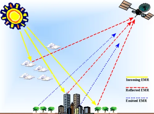
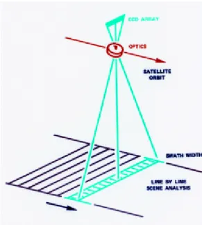
Figure 2.1 Data collection by remote sensing (from http://www.cla.sc.edu/geog/cgisrs/).

... 8

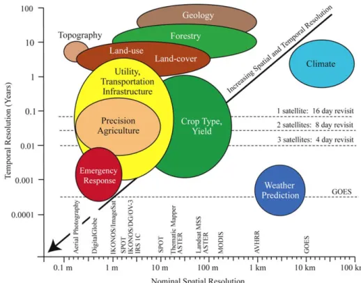
Figure 2.2 Spatial and temporal resolution for selected remote sensing applications (from Jensen, 2007). ... 10

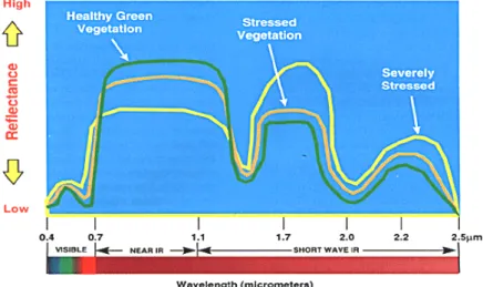
Figure 2.3 Spectral reflectance of vegetation (from http://www.csc.noaa.gov/products/sccoasts/html/images/reflect2.gif ). ... 11

Figure 2.4 Spectral reflectance of vegetation, soil and water (from http://landsat.usgs.gov/resources/remote_sensing/remote_sensing_applications.php )... 12

Figure 2.5 Conventional definitions for the three attitude axes of a sensor platform (source: Schowengerdt, 1997) ... 16

Figure 2.6 Ellipsoid, geoid and topographic surfaces (source: http://www2.uefs.br/geotec/topografia/apostilas/topografia(1).htm ) ... 19

Figure 2.7 The UTM Zone 29 (source: www.isa.utl.pt/der/Topografia/cartografia2.ppt) ... 20

Figure 2.8 Picture of the satellite SPOT 4. (from http://medias.obs-mip.fr/www/Reseau/Lettre/11/en/systemes/vegetation.html). ... 25

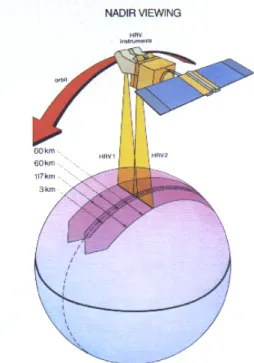
Figure 2.9 The cross-track direction operating mode of the two HRV sensors. (from http://www.spotimage.fr/html/_167_224_230_.php)... 27

Figure 2.10 Repeated observation by SPOT. (from http://www.spotimage.fr/html/_167_224_230_.php)... 27

Figure 2.11 The push broom principle (http://spot4.cnes.fr/spot4_gb/index.htm )... 28

Figure 2.12 SPOT’s Field of view. (from http://spot5.cnes.fr/gb/satellite/42.htm ) ... 28

Figure 2.13 The VEGETATION field of view. (from http://spot5.cnes.fr/gb/ ... 29

Figure 3.1 Reflectance from different wavelengths and different surfaces... 35

Figure 3.2 Monthly anomalies of NDVI over Europe for August 2003. Anomalies were computed with respect to the base period 1999-2004 (excluding 2003)... 39 Figure 3.3 As in Figure 3.2 but respecting to FAPAR anomalies. Anomalies were

top panel), an arable land pixel located in North Alentejo (right top panel), a coniferous forest pixel (left bottom panel) and a broad-leaved forest pixel (right bottom panel). Green dots and the solid curve respectively represent the time series of corrected and non-corrected NDVI monthly values. ... 43 Figure 3.5 Number of months between September 2001 and August 2002 that are

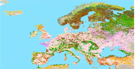
characterised by NDVI anomaly values below -0.025, using non-corrected (left panel) and corrected (right panel) NDVI data... 44 Figure 3.6 The Global Land Cover 2000 Project. ... 46 Figure 3.7 The updated version of the GLC2000 map for the European Window.

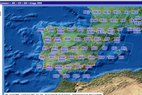
(http://www-gvm.jrc.it/glc200 ). ... 47 Figure 3.8 Landsat 7 imagery for the updating CLC, using the IMAGINE2000 software. (http://image2000.jrc.it/ )... 48 Figure 3.9 Corine Land Cover 2000 map for Portugal, as developed by ISEGI and the adopted 44 class-nomenclature (http://terrestrial.eionet.europa.eu/CLC2000)... 49 Figure 3.10 Corine Land Cover 2000 map for Portugal; the original map at 250m

resolution (left panel), the degraded map at 1000m resolution using the nearest neighbour technique (central panel), the degraded map at 1000m resolution using the majority rule (right panel)... 50 Figure 3.11 As in Figure 3.10 but respecting to a box centred in the Tagus estuary. .... 51 Figure 3.12 Histogram of relative frequencies of pixels in the 250m original map (blue), and in the 1000m degraded maps as obtained using the nearest neighbour technique (green) and the majority rule (red). Labels in bars identify classes referred to in the text. ... 51 Figure 3.13 Spatial distribution of relative presence for a set of five GLC2000 classes for the 1000m degraded maps using the majority rule, respectively urban areas (code 1.1.2), non irrigated arable land (code 2.1.1), broad-leaved forest (code 3.1.1), water courses (code 5.1.1) and estuaries (code 5.2.2)... 52 Figure 3.14 Patterns of simple correlation computed over the period 1982-2002 of

three-monthly averages of winter NAO (JFM) vs. winter precipitation (top panel) and surface air temperature (bottom panel)... 56

Figure 4.1 Interannual variability of late winter NAO index over the 21-year long period, from 1982 to 2002. Open (black) circles indicate years characterised by NAO indices above (below) the 3rd (1st) quartile. ... 60 Figure 4.2 Temporal averages of NDVISPR (left panel) and NDVISUM (right panel) over

the period from 1982 to 2002. Gray pixels over land correspond to areas covered by snow and ice. ... 61 Figure 4.3 As in Figure 4.2 but for PNAO (left panel) and TNAO (right panel). ... 62

Figure 4.4 Point correlation fields of NAO vs. NDVISPR (left panel) and NAO vs.

NDVISUM (right panel) over the period from 1982 to 2002. Black frames identify

the Baltic region and the Iberian Peninsula. The colorbar identifies values of correlation and the two arrows indicate the ranges that are significant at 5% level.

... 63 Figure 4.5 Boxplots of simple correlation between three months composite of North

Atlantic Oscillation (NAO) and NDVI for the 2 selected areas (NE and IB). ... 64 Figure 4.6 Seasonal anomalies of NDVISPR for 1986 (NAO+), 1995 (NAO-) and for

differences between 1995 and 1986 (upper, middle and lower panels, respectively) over IB and NE (left and right panels respectively). ... 65 Figure 4.7 Point correlation fields of NAO vs. TNAO (left panel) and NAO vs. PNAO

(right panel) over the period from 1982 to 2002. The colorbar shows values of correlation and the two arrows indicate the ranges that are significant at 5% level.

... 66 Figure 4.8 Geographical distribution of sets of selected pixels over the IB (upper

panels), based on the strong values of correlation of NDVISPR (upper left panel)

and NDVISUM (upper right panel) with NAO. Red, green and blue pixels are

respectively associated to forest and shrub, cultivated areas and other types of vegetation cover. Land cover type (low panel) as obtained from GLC2000) ... 68 Figure 4.9 As in Figure 4.8 but respecting to NHCP over NE. Red, green and blue

pixels are respectively associated to needle-leaved, evergreen, cultivated and other types of vegetation cover... 69 Figure 4.10 Dispersion diagrams of NDVISPR (upper panels) and NDVISUM (lower

panels) vs. PNAO (left panels) and TNAO (right panels) for selected pixels over the

IB. Each dot represents a pair of median values of a given set of selected 500 pixels, for a given year of the considered period (1982-2002). Years that belong to

-Figure 4.11 As in -Figure 4.10, but respecting to NE... 72 Figure 4.12 Annual cycles of monthly values of NDVI for NAO High Correlation

Pixels (NHCP), for spring (upper panel) and summer (lower panel), over IB (left panel) and NE (right panel). The annual cycles of average NDVI values for the entire period (1982-2002) are represented by thick solid lines, whereas the annual cycles of averages for the NAO- (NAO+) subsets are identified by the thin solid (dashed) curves. Vertical dashed curves delimit the season of the year... 74 Figure 4.13 As in Figure 4.12, but restricting to the annual cycles of NDVI for the

individual years of 1986 (NAO−) and 1995 (NAO+), respectively represented by the dashed and the solid lines. ... 74 Figure 5.1 Comparison of AVHRR, SPOT and MODIS VIs over Southeastern,

Australia, for February 2003 (Justice, 2005)... 80 Figure 5.2 Time series of annual wheat yield in Portugal for the period from 1961 to

2005: yield (solid line), general trend (dashed line) and anomalies for detrended time series (line with asterisks). ... 84 Figure 5.3 Contribution of different growing regions of Portugal to total wheat yield for the period from 1996 to 2003. ... 84 Figure 5.4 Percentage of Alentejo’s wheat yield for hard and soft wheat for the period from 1996 to 2003 ... 85 Figure 5.5 Patterns of simple correlation between spring NDVI composites and wheat yield in Portugal, for the period of 1982-1999 (left panel); patterns of simple correlation that are significant at the 99% level (right panel). ... 86 Figure 5.6 Pixels coded as “arable land not irrigated” according to Corine2000 for

Portugal. (left panel). Relative frequency of correlation coefficient values between spring composite of NDVI and wheat yield in Portugal, for pixels coded as arable land (right panel). ... 87 Figure 5.7 As in Figure 5.5 (left panel), but for the pixels with correlations that are

significant at the 99% level. ... 87 Figure 5.8 Time series for the period 1982-1999 of detrended anomalies of wheat yield in Portugal (green curve) and of spring NDVI averaged over the “wheat-like” pixels (red curve). Values of wheat yield were normalized by subtracting the mean and dividing by the standard deviation... 88

Figure 5.9 Patterns of simple correlation between wheat yield in Portugal and the three most relevant meteorological fields for the period of 1982-1999; top panel: net short wave radiation; middle panel: surface air temperature; bottom panel: precipitation. Boxes in the Southern sector delimit the area containing “wheat-like” pixels... 90 Figure 5.10 Patterns of simple correlation, over the Iberian Peninsula, between NAO

averaged for April, May and June and contemporaneous fields of radiation (left panel), temperature (central panel) and precipitation (right panel) for the considered period 1982-1999. ... 91 Figure 5.11Patterns of simple correlation between wheat yield in Portugal and the three most relevant meteorological fields for the period of 1982-1999; top panel: net long wave radiation; middle panel: surface air temperature; bottom panel: precipitation... 92 Figure 5.12 Time series (1982-1999) of observed (green curve) wheat yield in Portugal and of corresponding modeled values (red curve) when using a linear regression model based on spring NDVI and NAO in June (upper panel). Time series (1982-1999) of residuals and respective 95% level confidence intervals (central panel); the single outlier (in 1998) is highlighted in red. Time series (1982-1999) of observed (green curve) wheat yield in Portugal and of corresponding modeled values (red curve) as obtained from the leave-one-out cross-validation procedure.

... 94 Figure 6.1 Monthly time-series (1999–2006) of NDVI averaged over Continental

Portugal for all pixels (black line), for pixels of non-irrigated arable land (red line) and of pixels of broad-leaved forest (green line). Black arrows indicate the drought episodes of 1999, 2002 and 2005. ... 99 Figure 6.2 Monthly means of NDVI (1999-2006) over Continental Portugal, covering

the period from September to August... 100 Figure 6.3 NDVI anomalies from September to August respecting to the year of

1998/1999. ... 102 Figure 6.4 As in Figure 6.3 but respecting to the year of 2001/2002... 103 Figure 6.5 As in Figure 6.3 but respecting to the year of 2004/2005... 104 Figure 6.6 Monthly time-series (1992–2005) of SWI averaged over Continental

Figure 6.8 Climatological cycle of SWI vs. NDVI. Letters indicate months of the year. ... 108 Figure 6.9 SWI anomalies for January to August respecting to the year 1998/1999. .. 109 Figure 6.10 As in Figure 6.9 but respecting to the year 2004/2005. ... 110 Figure 6.11 Annual cycles (red curves) of SWI vs. NDVI for the drought episodes of

1999 (left panel) and 2005 (right panel). The climatological cycle (black curves) is also presented for reference purposes... 111 Figure 6.12 Annual cycles of spatially averaged NDVI for each year of the considered period (1999-2006) over non-irrigated arable land (top panel) and coniferous forest (bottom panel). The drought episodes of 1999 and 2005 are represented, respectively, by the curves with circles and asterisks. The line in bold refers to monthly means over the entire period. ... 112 Figure 6.13 Percentage of continental Portugal with monthly NDVI anomalies lower

than 0 (red bars) and lower than -0.025 (green bars), from September to August of 2005. The black line represents the percentage of mainland affected by extreme drought, i.e., with PDSI ≈ -4. The 3-month delay of PDSI relatively to NDVI (as indicated by the two different horizontal time axes) is worth being noted. ... 114 Figure 6.14 Number of months between September and August that are characterised by NDVI anomaly values below -0.025, for each year of the considered period (1999-2006)... 116 Figure 6.15 As in Figure 6.14, but all pixels that are identify as burned areas are masked

... 121 Figure 7.1 Annual burned areas in Continental Portugal (right panel) for the fire season of 2003 (red pixels) using the criterion of at least 5 months of NDVI anomalies below -0.075 during the period from September to May of 2004; black pixels refer to burned scars for the previous fire season of 2002. Annual burned areas in Continental Portugal (central panel) for the period 2000-2004 as identified from Landsat imagery. The central panel was adapted from Pereira et al. (2006). ... 125 Figure 7.2 Annual burned areas in Continental Portugal (left panel) for the fire season of 2004 (red pixels) using the criterion of at least 5 months of NDVI anomalies below -0.075 during the period from September to May of 2005; black pixels refer to burned scars for the previous fire season of 2003. Annual burned areas in

Continental Portugal (central panel) for the period 2000-2004 as identified from Landsat imagery. Annual burned areas in Continental Portugal (right panel) for the fire season of 2004 (red pixels) using the criterion of at least 7 months of NDVI anomalies below -0.075 during the period from January to August of 2005; black pixels refer to burned scars for the previous fire season of 2003. The central panel was adapted from Pereira et al. (2006)... 126 Figure 7.3 Annual burned areas in Continental Portugal (left panel) for the fire season of 2005 (red pixels) using the criterion of at least 5 months of NDVI anomalies below -0.075 during the period from September to May of 2006; black pixels refer to burned scars for the previous fire season of 2004. Annual burned areas in Continental Portugal (central panel) for the year of 2005 as identified from Landsat imagery. Annual burned areas in Continental Portugal (right panel) for the fire season of 2005 (red pixels) using the criterion of at least 5 months of NDVI anomalies below -0.075 during the period from January to June of 2006; black pixels refer to burned scars for the previous fire season of 2004. The central panel is courtesy from J.M.C. Pereira. ... 127 Figure 7.4 Burned scars for each year of the period 1998-2005 as identified based on NDVI anomalies... 129 Figure 7.5 Time series of annual burned areas in Continental Portugal for the period

1998-2005 as obtained from the developed methodology (solid line) and based on DGRF information (dotted curve). ... 130 Figure 7.6 Time series of NDVI for selected pixels in a set of eight large fire scars, each one corresponding to an event that has occurred in a given year of the 1998-2005. The location of the selected fire scars is given in the upper panel. ... 132 Figure 7.7 Time series of averaged NDVI over three large fire scars, one of them

associated to an event in 2001 and the remaining associated to two events in 2003. The location of the selected fire scars is given in the upper panel. ... 133

L

IST OF

T

ABLES

Table 2.1 Regions used in remote sensing. (adapted from

http://www.esa.int/esaEO/SEMLFM2VQUD_index_1_m.html). ... 9

Table 2.2 Table of Ellipsoids (Adapted from http://ltpwww.gsf.nasa.gov/

IAS/handbook/hamdbook_htmls/chapter1/chapter1.html) ... 18 Table 2.3 Projection plane equations for several common map projections (Moik, 1980). The latitude of a point on the Earth is ϕ and its longitude is λ . The projected map coordinates, x and y, are called “easting” and “northing”, respectively. R is the equatorial radius of the Earth and ε is the Earth’s eccentricity. The subscripted values of latitude and longitude pertain to the definition of a particular projection (source: Schowengerdt, 1997)... 21 Table 2.4 HRV Spectral Bands.(from

http://www.spotimage.fr/html/_167_224_230_.php)... 25 Table 2.5 HRVIR Spectral Bands

(fromhttp://www.spotimage.fr/html/_167_224_230_.php)... 26 Table 2.6 Orbit characteristics for SPOT 5. ... 30 Table 2.7 SPOT 5 sensor characteristics. ... 30 Table 2.8 General time coverage by satellite. (from

http://www.ngdc.noaa.gov/stp/NOAA/noaa_poes.html)... 31 Table 2.9 NOAA Satellites Orbital Characteristics. (Adapted from

http://www.crisp.nus.edu.sg/~research/tutorial/noaa.htm )... 32 Table 2.10 AVHRR Sensor Characteristics. (from

http://www.crisp.nus.edu.sg/~research/tutorial/noaa.htm)... 33 Table 4.1 Descriptive statistics of the distributions of NDVI anomalies for the sets of selected pixels associated to forest and shrub, and to cultivated areas, in the cases of spring and summer over the Iberian Peninsula and the Baltic region. P1, Q1, Q2, Q3 and P99 respectively denote percentile one, the first quartile, the median, the third quartile and percentile 99. Percent figures in parenthesis below the land cover types indicate the fraction of pixels of the considered set associated to that type. 70

samples. ... 88 Table 5.2 Correlation coefficient values between annual wheat yield and monthly net

long wave radiation, air surface temperature and precipitation (from January to June) for the pixels coded as arable land not irrigated. Bold values are representing correlations values that are significant at 95% level and red value is presented the correlation value significant at 99% level. ... 89 Table 5.3 As in table 5.1, but respecting to net short-wave radiation, temperature,

precipitation in March and to NAO in June. ... 92 Table 6.1 Percentage of mainland Portugal stricken by serious drought, i.e., with

monthly NDVI anomalies below -0.025 in more than 9 months (out of 11). ... 115 Table 6.2 Total amounts and relative proportions of pixels affected by drought for

different land cover types during the drought episodes of 1999, 2002 and 2005. 115 Table 6.3 Cumulative effect of drought conditions for specific land cover types during the drought episodes of 1999, 2002 and 2005... 118 Table 7.1 Percentage of burned pixels for pixels classified as non irrigated Arable Land, Forest, Transitional woodland-shrub and Shrubland (using Corine Land Cover Map 2000, CLC2000) for the fire seasons from the years 1998 to 2005. ... 130

L

IST OF

A

CRONYMS

AVHRR Advanced Very High Resolution Radiometer CLC2000 Corine Land Cover 2000

CNES Centre National d'Etudes Spatiales

CORINE COoRdinate INformation on the Environment CRU Climate Research Unit

DFRF Direcção Geral dos Recursos Florestais EEA European Environment Agency

EMD Empirical Mode Decomposition ERS European Remote Sensing

FAO Food and Agriculture Organization GAC Global Area Coverage

GEWEX Global Energy and Water Cycle Experiment

GIMMS Global Inventory Monitoring and Modelling System GIS Geographical Information System

GLAM Global Agriculture Monitoring GLC2000 Global Land Cover 2000

GPCC Global Precipitation Climatology Centre HRPT High Resolution Picture Transmission HRV High Resolution Visible

HRVIR High Resolution Visible and Infrared

IB IBerian peninsula

IFOV Instantaneous Field of View INE Instituto Nacional de Estatística

ISEGI Instituto Superior de Estatística e Gestão da Informação JRC Joint Research Center

LAC Local Area Coverage

MODIS MODerate Resolution Imaging Spectroradiometer

MS MultiSpectral mode

MSU Microwave Sounding Unit

MVC Maximum Value Composite

NASA National Aeronautics and Space Administration NDVI Normalised Difference Vegetation Index

NDVISPR SPRing NDVI

NDVISUM SUMmer NDVI

NE Northeastern Europe

NHCP NAO High Correlated Pixels NAO North Atlantic Oscillation

NIMA United States National Imagery and Mapping Agency

NIR Near InfraRed

NOAA US National Oceanic and Atmospheric Administration

PAN PANchromatic mode

PDSI Palmer Drought Severity Index

PNAO Precipitation corresponding to the winter NAO index

SPOT Satellite Pour l’Observation de la Terre

SWI Soil Water Index

SWIR ShortWave InfraRed

TIR Thermal InfraRed

TNAO Temperature corresponding to the winter NAO index

TOVS TIROS Operational Vertical Sounder

USDA/FAS United States Department of Agriculture/Foreign Agricultural Service

UTM Universal Transverse Mercator

VGT VEGETATION

VGT-NDVI NDVI using VGT VGT-P VGT Physical products VGT-S VGT Synthesis products

VI Vegetation Index

VIS VISible

WCRP World Climate Research Program WMO World Meteorological Organization

1. I

NTRODUCTION

Terrestrial ecosystems are of primary importance as they exert control and can partially drive the climate system at the global scale. Among other climate related impacts, terrestrial ecosystems are responsible for the storage and release of greenhouse gases, such as carbon dioxide (CO2), methane and nitrous oxide. However terrestrial

ecosystems themselves are subject to the influence of local climate, leading to a multiplicity of feedback mechanisms between carbon cycle and climate, which may in turn be attenuated or intensified by regional and global climate variability. The role played by vegetation becomes decisive in this context because of the large quantities of carbon that are stored in vegetation and organic matter. When released into the atmosphere, in CO2 form, stored carbon may have strong impacts on global climate.

Since carbon discharges, such as those resulting from the combustion of fossil fuel and in land-use changes, are mainly due to human activities, forest has become a major carbon source either in a direct or in an indirect way.

As carbon changes are a major driver of climate change, it has become essential to understand in detail how terrestrial ecosystems may gain carbon through photosynthesis and lose it via autotrophic and heterotrophic respiration (as well as by volatile organic compounds, methane and dissolved carbon, in less but not neglected amounts). Quantifying and predicting the carbon cycle and modelling climate feedbacks is not an easy task, mainly because of the present limited knowledge about the geobiochemical processes that transform/recycle the carbon inside the climate system (Heimann and Reichstein, 2008).

In recent years a growing number of works has provided strong evidence that the terrestrial components of the carbon cycle are responding to global climate changes and trends. Heimann and Reichstein (2008) have shown that the strong interannual variability of globally averaged growth rate of atmospheric CO2 is highly correlated

impact of extreme events on the health of vegetation of Western Amazonia and Southeastern Asia, leading to a loss of carbon by forest due to the decrease of photosynthetic productivity and/or increase in respiration. In this context, when studying the climate impact on carbon budget it is usually assumed that the CO2 uptake,

by photosynthesis, is stimulated by the increases in both the CO2 itself and in

temperature (Davidson and Janssens, 2006). These processes that essentially occur in boreal forests and temperate regions are expected to saturate at high values of CO2

concentration and temperature. On the other hand, respiration responds exponentially to temperature changes, but is not sensitive to CO2 levels. This may indicate that the

biosphere provides a negative feedback to the increase of temperature and CO2 until

temperature is so high that the stimulation of respiration exceeds the fertilization effect of CO2. However the full process may be even more complex if we take into account

the complex mechanisms that occur in soil layers. Furthermore, other climatic and environmental factors may modify the carbon balance (Denman et al, 2007).

The primary productivity in the majority of the terrestrial ecosystems is limited by water availability, which means that significant changes in precipitation may have a strong impact on the dynamics of the carbon cycle. Changes in frequency and occurrence of precipitation (even without changes in the total annual amount) may be decisive to photosynthetic productivity because the precipitation regime determines when the water will be used and transpired by vegetation or just runoff and evaporate (Knapp et al., 2002). On other hand, in a warmer Earth, an increase of evaporation is expected, leading to a negative water balance, whereas the diminishing of loss of water by plant stomata in a world with a surplus of CO2 will mitigate the previous effect. As a

consequence, the net result will mainly depend on the water holding capacity of the soil, as well as on the vertical distribution of carbon and roots in the soil and on the general sensitivity of vegetation to drought (Heimann and Reichstein, 2008). Water limitations may even suppress the response of respiration to temperature (Reichstein et al., 2007). Under drier conditions, some climate change scenarios give an indication of an increasing of carbon sequestration, by respiration suppression, as well as of a reducing of carbon loss due to the decrease of photosynthetic productivity (Ciais et al., 2005; Saleska et al., 2003).

It is a well establish fact that the biosphere does not solely respond to changes in average climatic variables, but its changes are mainly associated to fluctuations and to variability of climatic variables, which in turn are related to the occurrence of extreme

events. A good example was the recent heat wave that stroke Europe during the summer of 2003; the carbon sequestration that occurred in the previous five years was annihilated in just a few days of extreme weather conditions. Ciais et al. (2005) have shown that, rather than accelerating with temperature rise, respiration has decreased together with productivity. These authors have highlighted that droughts and heat waves may modify the health and productivity of vegetation and transform, albeit for a short period, sinks into sources, leading to a short-term positive carbon-climate feedback. It may be noted that these mechanisms are related to the productivity rates of cultures, mainly in regions where artificial irrigation is not employed and for crops with vegetative cycles that do not coincide with the extreme heat. The negative effects of such extreme events may be even amplified by lagged impacts, such as those associated to tree death and the slow recovery of vegetation in case of wildfires (Holmgren et al., 2006; Heimann and Reichstein, 2008, Le Page et al., 2008).

Changes in temperature seasonality may have induced the occurrence of mild winters and early springs in high latitudes, leading to an early melting and flowering and, consequently, to a higher vulnerability to frost (Myneni et al., 1997; Zhou et al., 2001). On the other hand, the observed increases of temperature in spring and autumn over high latitude regions of the Northern Hemisphere leads inevitably to larger growing seasons and to higher photosynthetic activity and therefore strongly affecting the carbon seasonal cycle. However the processes that take place in spring and in autumn have a different nature. Whereas in spring photosynthesis dominates respiration, the opposite takes place in autumn and therefore it is in spring that an increase in CO2

sequestration is expected to occur (Piao et al., 2008). Accordingly, in the future and in case the autumn warming occurs faster than the spring warming, the ability of carbon sequestration by Northern ecosystems may decrease faster than previously suggested (Sitch et al., 2008). However, changes in the seasonality of temperature and precipitation may have distinct impacts, depending on local characteristics.

Temporal changes in wind speed, air temperature, water stress and humidity may change the frequency and severity of wildfires with the consequent release, in a few minutes, of enormous quantities of carbon, into the atmosphere, that have been accumulated in soil and vegetation during centuries (Shakesby et al., 2007; Michelsen et al., 2004). More frequent and intense forest fires reduce biomass and productivity of the surface layer of soil, leading to erosion and decrease of biodiversity and finally to soil

summers drought; persistent droughts tend to intensify land degradation due to land use pressure, setting conditions, when rainfall starts, for the spreading and for a faster growing of highly flammable wild plants (Dube, 2007; Holmgren and Scheffer, 2001). In arid and semi-arid regions, and during dry periods, the highly flammable herbaceous species tend to compete with native vegetation. With the increase of meteorological fire risk, these areas tend to become more vulnerable to wildfires, due to the accumulation of highly flammable dry biomass. Repeated fires may in turn induce changes in vegetation structure, by converting the native vegetation into shrub-woodland vegetation (Brooks and Pyke, 2002; Sheuyange et al., 2005).

A solid understanding of vegetation dynamics and climate variability becomes therefore crucial for the integration of the carbon cycle into the climate system and for the establishment of links between land use changes and extreme events, namely droughts and wildfires. In such a wide and complex context, remote sensing has become a very useful tool to monitor, at the global scale and relatively low cost, vegetation dynamics and stress, as well as deforestation and land use changes. The emergence of new satellite platforms and sensors, has prompted a strong effort to develop more sophisticated methods and algorithms to homogenise time series and to integrate observation of different nature. A good example is the one provided by the Global Inventory Monitoring and Modelling System (GIMMS) group, that has supplied the user community with more than twenty years of remote-sensed data at 8 km resolution, based on original information from the successive satellites of the AVHRR/NOAA series. Europe has built another complementary important initiative, the VEGETATION system that, since the end of 1998, has been supplying data on earth surface characteristics, at 1 km resolution, based on remote sensed information from VEGETATION instrument on board of the French SPOT satellites. An effort has also been put into the development of several vegetation indices, specifically design to quantify concentrations of green leaf vegetation and identify places where vegetation is either healthy or under stress.

The aim of the present thesis is to further investigate the relationship between climate variability and vegetation dynamics in Europe by combining remote-sensed information and meteorological data. Special attention will be devoted to the Iberian

Peninsula and Portugal and the study will encompass different aspects of the problem, from the impact of NAO on the vegetative cycle to vegetation recovery after fire events.

The thesis is organised into three main parts; a first one dedicated to fundamentals, data and methods; a second one dealing with the impact of climate variability on vegetation dynamics in Europe and crop production in southern Portugal; and a third focusing on the effects of extreme events on Portuguese vegetation health.

The first part comprises Chapters 2 and 3. In Chapter 2 an overview is given on remote sensing and image correction techniques and a detailed description is provided about the major characteristics of NOAA and SPOT systems. Chapter 3 gives a thorough description of datasets used, namely remote-sensed (GIMMS, VITO, CLC2000, GLC2000) and meteorological (CRU, GPCC) data and presents an overview on the characteristics and the applicability of vegetation indices, namely on the Normalised Difference Vegetation Index (NDVI).

The second part comprises Chapters 4 and 5 and the goal is to assess the impact of climate variability on vegetation dynamics and crop production. Chapter 4 is dedicated to the analysis of the relation between vegetation phenology and climate variability over Europe and to characterizing the response of vegetation to both precipitation and temperature in two contrasting areas of Europe, respectively Northeastern Europe and the Iberian Peninsula. The impact of the Northern Atlantic Oscillation (NAO) on the vegetative cycle in the two regions is assessed and related to the different land cover types and to the respective responses to climate variability. Results of this chapter have been published in Gouveia at al. (2008). Chapter 5 gives a brief description of the impact of climate variability on wheat production and yield that is mostly relevant in southern Portugal. The role of relevant meteorological variables is investigated, namely net solar radiation, temperature and precipitation and the impact of NAO is evaluated. A simple regression model of wheat yield is built up using as predictors spring NDVI and NAO in June that are related to meteorological conditions during the growing and maturation stages of wheat. Parts of these results have been published in Gouveia and Trigo (2008).

The third part of the thesis which comprises Chapters 6 and 7 is related to the assessment of the impact of extreme events, such as drought episodes and wildfires, on vegetation health in Continental Portugal. Chapter 6 is dedicated to the spatial and temporal monitoring of heat and water stress of vegetation. The severity of a given

well as to those of 1999 and 2002. Parts of these results have been submitted in Gouveia et al.*, (2008). In Chapter 7 a simple methodology is presented that allows identifying burned areas based on the analysis of persistent negative anomalies of NDVI. The developed methodology allows evaluating the susceptibility to fire of different land cover types as well as assessing the distinct recovery profiles of vegetation after wildfire events.

Finally an overview of results is given in Chapter 8 and a summary of the most important conclusions are presented on the work that was performed.

*Gouveia, C., DaCamara, C.C. Trigo; R.M., 2008: Drought and Vegetation Stress Monitoring in Portugal using Satellite Data, Natural Hazards and Earth System Sciences (Submitted).

2. F

UNDAMENTALS

2.1

Remote sensing

Following the American Society of Photogrammetry and Remote Sensing we will adopt a combined definition of photogrammetry and remote sensing (Colwell, 1997), that will be defined as

“the art, science, and technology of obtaining reliable information about physical objects and the environment, through the process of recording, measuring and interpreting imagery and digital representations of energy patterns derived from noncontact sensor systems”.

This is a complex and comprehensive sequence of processes involving the detection and measurement of electromagnetic radiation of different wavelengths reflected or emitted from distant objects or materials, with the aim of estimating their physical and biophysical properties and/or organising them in terms of class/type, substance, and spatial distribution. A device such as a camera or a scanner that is able to detect the electromagnetic radiation reflected or emitted from an object is called a "remote sensor" or "sensor". The vehicle, such as an aircraft or a satellite that carries the sensor is called a "platform".

Remote sensing aims therefore at identifying and describing objects and/or environmental conditions by analysing the respective signatures on the reflected and emitted spectra of electromagnetic radiation (Figure 2.1). Because of the unique view it provides of the Earth, remote sensing has come to be a very important method to analyse the environment. In this sense, remote sensing is an exploratory science, as it provides images of areas in a fast and cost efficient way, and attempts to uncover the properties of the observed elements.

Figure 2.1 Data collection by remote sensing (from http://www.cla.sc.edu/ geog/cgisrs/).

2.2

Radiometric concepts

All matter reflects, absorbs and emits electromagnetic radiation in a unique way. For example, the reason why a leaf looks green is that the chlorophyll absorbs blue and red and reflects green radiation. Such unique characteristics of matter are usually called spectral characteristics.

The flux of electromagnetic radiation is usually characterised by the so-called radiance, L, which is defined as the flux per unit projected area (at the specific location in the plane of interest) per unit solid angle (in the direction specified relative to the reference plane). The SI units of radiance are therefore Wm-2sr-1.

In general, we may consider that:

where:

L is the radiance recorded within the Instantaneous Field of View (IFOV) of the considered optical remote sensing system, i.e., the area from which radiation impinges on the detector (e.g. a picture element or pixel in a digital image)

(

Ω

)

=

f

,

s

,

t

,

,

P

,

and where:

λ denotes wavelength (i.e. the spectral response measured in various bands or at specific frequencies);

sx,y,z denotes the size of the picture element (or pixel) whose location is at (x,y,z);

t refers to temporal information (i.e., when and how often the information is acquired);

θ

P denotes the polarization of back-scattered energy recorded by the sensor;

Ω denotes the radiometric resolution (precision) at which the data (e.g., reflected, emitted, or back-scattered radiation) are recorded by the remote sensing system.

As shown in Table 2.1, the electromagnetic radiation regions used in remote sensing are the near ultra-violet (0.3-0.4 μm), the visible (0.4-0.7 μm), the reflective infrared (0.7-3.0 μm), the thermal infrared (3.0-14 μm) and the microwave (1 mm-1 m). The spectral range of reflective infrared is more influenced by solar reflection than by the emission from the ground surface. The reflective infrared is usually subdivided into the near infrared (0.7-0.9 μm) and the shortwave infrared (0.9-3.0 μm). In the thermal infrared region, emission from the surface dominates the radiant energy with little influence from solar reflection.

Table 2.1 Regions used in remote sensing. (adapted from

http://www.esa.int/esaEO/SEMLFM2VQUD_index_1_m.html).

Ultra-violet Visible Infrared Microwave

0.30-0.40μm Near ultra-violet 0.40-0.45 μm Violet 0.7-3.0 μm Reflective Infrared 1mm-1m 0.45-0.50 μm Blue 3.0-14 μm Thermal Infrared

0.50-0.55 μm Green 14.0- 1000 μm Far Infrared

0.55-0.60 μm Yellow

0.60-0.65 μm Orange

Meteorological, agricultural and environmental remote sensing in general is commonly performed in the visible (VIS), the near-infrared (NIR), the shortwave infrared (SWIR) and thermal infrared (TIR) portions of the spectrum.

Resolution is generally defined as the ability of an entire remote-sensing system to render a sharply defined image. Resolution involves the following specific types (Figure 2.2)

• Spatial resolution, defined as the size of the field-of-view (FOV), e.g., 10 × 10 m;

• Spectral resolution, defined as the number and size of spectral regions the sensor records data, e.g. blue (B), green (G), red (R), NIR, TIR, microwave;

• Temporal resolution which is related to how often the sensor acquires data, e.g. every 30 days;

• Radiometric resolution, defined as the sensitivity of detectors to small differences in electromagnetic energy.

Figure 2.2 Spatial and temporal resolution for selected remote sensing applications (from Jensen, 2007).

It may be noted that the resolution determines how many pixels are available in measurement, but more importantly, higher resolutions are more informative, giving more data about more points. However, more resolution occasionally yields less data. For example, in thematic mapping to study plant health, imaging individual leaves of plants is actually counterproductive. Also, large amounts of high-resolution data can clog a storage or transmission system with useless data, when a few low-resolution images might be a better use.

Reflectance is defined as the ratio of incident flux on a sample surface to reflected flux from the surface and ranges between 0 and 1. Reflectance with respect to wavelength is called spectral reflectance. Figure 2.3 shows an example of spectral reflectance for vegetation. Spectral reflectance is assumed to be different with respect to the type of land cover. This feature in many cases allows the identification of different land covers types with remote sensing by observing the spectral reflectance or spectral radiance from the surface. Figure 2.4 shows three curves of spectral reflectance for typical land covers; vegetation, soil and water. As seen in the figure, vegetation has a very high reflectance in the near infrared region, though there are three low minima due to absorption.

Figure 2.3 Spectral reflectance of vegetation (from http://www.csc.noaa.gov/

Figure 2.4 Spectral reflectance of vegetation, soil and water (from

http://landsat.usgs.gov/resources/remote_sensing/remote_sensing_applicati ons.php).

Soil has rather higher values for almost all spectral regions. Water has almost no reflectance in the infrared region. Chlorophyll, contained in a leaf, has strong absorption at B (0.45 μm) and R (0.67 μm), and high reflectance at NIR (0.7-0.9 μm). This characteristic reflects in the small peak at G (0.5-0.6 μm), which makes vegetation green to the human observer. NIR is very useful for vegetation surveys and mapping because such a steep gradient at 0.7-0.9 μm is produced only by vegetation. Because of the water content in a leaf, there are two absorption bands at about 1.5 μm and 1.9 μm. This is also used for surveying vegetation greenness.

2.3

Image correction

2.3.1 Atmospheric correction

Radiation from the Earth's surface undergoes significant interaction with the atmosphere before it reaches the satellite sensor. This interaction with the atmosphere can be severe, as in the case of cloud contamination, or minor, as in the case when the FOV is essentially a clear sky (Schott and Henderson-Sellers, 1984). Regardless of the

type of analysis that is performed on the remotely sensed data, it is important to understand the effects of the atmosphere upon the radiance response.

The propagation of electromagnetic radiation through the atmosphere is affected by two essential processes; absorption and scattering. Absorption occurs when a fraction of energy passing through the atmosphere is absorbed by some of the atmospheric constituents and is then re-emitted at different wavelengths. Scattering occurs when a fraction of energy passing through the atmosphere has its direction altered through a diffusion of radiation by small particles in the atmosphere. The type and significance of the scattering depends upon the size of the scattering element compared to the wavelength of the radiation (Schott and Henderson-Sellers, 1984; Drury, 1987).

At the shorter wavelengths, attenuation occurs by scattering due to clouds and other atmospheric constituents, as well as by reflection. The effect of scattering on the visible wavelengths is significant and must be compensated for when developing empirical relationships through time. The most significant interaction that thermal infrared radiation undergoes, as it passes through the atmosphere, is by absorption, primarily due to ozone and water vapour particles in the atmosphere.

The objective of atmospheric correction is to retrieve the surface reflectance (that characterizes the surface properties) from remotely sensed imagery by removing the atmospheric effects. Since atmospheric correction has been shown to significantly improve the accuracy of image classification, the problem has received considerable attention from researchers in remote sensing who have devised a number of approaches to its solution (Crippen, 1987). Most of them are sophisticated approaches (based on e.g. correlation with ground-based measurements, ground truth methods, in-scene methods, multiple view angle, multiple altitude techniques, atmospheric propagation models) but they are computationally challenging and have only been validated on a very small scale. Simplified approaches (e.g. use of a constant correction factor for each channel of the dataset) have also been adopted, especially in cases of operational applications over large areas. Atmospheric correction is beyond the scope of this work and an overview of methods is given e.g. in Chapter 6 of Schott (1997).