UNIVERSIDADE DE LISBOA
FACULDADE DE CIÊNCIAS
DEPARTAMENTO DE ESTATÍSTICA E INVESTIGAÇÃO OPERACIONAL
The impact of heatwaves on mortality in the Lisbon district –
ICARO system revisited
Maria Carolina Serrão Nogueira Nascimento Bulhosa
Mestrado em Bioestatística
Relatório de Estágio orientado por:
Professora Doutora Marília Antunes
Agradecimentos
Gostaria de agradecer, em primeiro lugar, aos meus orientadores, Professora Mar´ılia Antunes e Doutor Baltazar Nunes, por me terem possibilitado a realizac¸˜ao deste trabalho de est´agio e guiado ao longo de todo o processo. N˜ao posso deixar de agradecer `a Susana Silva, que n˜ao sendo oficialmente minha orientadora, foi sempre de uma dedicac¸˜ao e ajuda preciosas.
Gostaria de agradecer tamb´em a todos os colegas do Departamento de Epidemiologia do Instituto Nacional de Sa´ude Doutor Ricardo Jorge, por me terem acolhido t˜ao amigavelmente durante estes meses. Um especial muito obrigada `a Inˆes Batista. Ao Constantino, o meu obrigada por toda a ajuda na programac¸˜ao.
Quero ainda agradecer aos meus colegas de curso, por toda a amizade e colaborac¸˜ao ao longo destes dois anos.
Por fim, mas de extrema importˆancia, o meu eterno obrigada `a minha fam´ılia e amigos mais pr´oximos, por todo o apoio emocional e n˜ao s´o. Aos meus pais, M´arcio, Marta, Isabel, Sofia, Rita, Pedro e Jo˜ao, muito obrigada!
Resumo
A temperatura ´e um fator ambiental com influˆencia direta no conforto e sa´ude humana. Sabe-se que diferentes populac¸˜oes est˜ao adaptadas a diferentes climas, consoante as regi˜oes onde vivem, e que se adaptam inclusive `as alterac¸˜oes sazonais que ocorrem ao longo do ano, tornando-se mais tolerantes ao frio ao longo do inverno e ao calor ao longo do ver˜ao. Ainda assim, temperaturas extremas (tanto quentes como frias) podem causar um aumento da mortalidade. Normalmente a mortalidade ´e mais elevada no inverno do que no ver˜ao, embora esporadicamente ocorram picos de mortalidade durante alguns ver˜oes, que podem ser explicados por calor extremo. O foco deste trabalho ser´a este excesso de mortalidade associada a calor extremo no distrito de Lisboa.
O estudo do efeito que o excesso de calor tem sobre a mortalidade ´e de extrema importˆancia hoje em dia, tendo em conta o per´ıodo de alterac¸˜oes clim´aticas em que vivemos - que est´a a provocar o au-mento das temperaturas e a intensidade e frequˆencia de fen´omenos extremos, como subidas s´ubitas da temperatura e ondas de calor – e tamb´em devido ao aumento de certos fatores de risco que aumentam a vulnerabilidade da populac¸˜ao ao calor, nomeadamente a crescente urbanizac¸˜ao e envelhecimento da populac¸˜ao portuguesa. Assim, a relac¸˜ao entre a temperatura e a mortalidade em Portugal deve ser pro-fundamente estudada, de modo a tentar prever e atenuar as consequˆencias do aquecimento global, com especial atenc¸˜ao `a populac¸˜ao mais vulner´avel e com menos capacidades de adaptac¸˜ao.
Em Portugal, o excesso de calor nos ver˜oes de 1981 e 1991 provocou um n´umero de mortes muito acima do n´umero de mortes esperadas, que poderia ter sito evitado, pelo menos em parte, caso existisse algum sistema de aviso e resposta a emergˆencias relacionadas com o calor. Surgiu assim a necessidade de se desenvolver um sistema de alerta e vigilˆancia de calor, com o objetivo de mitigar esse efeito. Desta forma, criou-se em 1999 o sistema ´ICARO – Importˆancia do Calor: Repercuss˜ao sobre os ´Obitos -, que funciona desde ent˜ao entre os meses de maio e setembro, visando monitorizar e alertar para poss´ıveis aumentos de mortalidade causados por calor extremo. Para isso foi inicialmente criado um modelo estat´ıstico de s´eries temporais com um limiar dinˆamico, calibrado para o distrito de Lisboa, considerando os dados relativos `as ondas de calor de 1981 e 1991: modelo ´ICARO Lisboa. Este modelo identifica bem os per´ıodos de calor extremo com impacto sobre a mortalidade. No entanto, por um lado, sobrestima alguns dos aumentos de mortalidade, dando origem a falsos alarmes e, por outro lado, subestima os impactos tardios de ondas de calor mais prolongadas.
O objetivo deste trabalho ´e, assim, formular um novo modelo estat´ıstico que relacione o calor e a mortalidade com o mesmo grau de sensibilidade, mas maior especificidade que o modelo ´ICARO Lisboa. Esse novo modelo ser´a ent˜ao desenvolvido e depois comparado com o modelo ´ICARO, com vista a optimizar/atualizar o sistema de vigilˆancia.
Sendo que o efeito das temperaturas adversas sobre a mortalidade n˜ao ´e imediato, podendo prolongar-se no tempo ao longo de v´arios dias, este deve prolongar-ser explicado pela combinac¸˜ao de exposic¸˜oes ao longo de v´arios momentos do passado, dependendo simultaneamente da intensidade e do momento das exposic¸˜oes ao calor. Desenvolveu-se ent˜ao um modelo n˜ao linear de desfasamentos distribu´ıdos (DLNM –
dis-que permite predizer de forma mais eficaz o efeito atrasado dis-que o calor pode causar na mortalidade, bem como o seu efeito cumulativo. Os DLNM baseiam-se numa func¸˜ao bidimensional, denominada “cross-basis”, que descreve simultaneamente as dependˆencias de exposic¸˜ao-resposta ao longo do espac¸o da temperatura e ao longo da sua estrutura temporal. Deste modo, o efeito de cada exposic¸˜ao at´e um de-terminado atraso – lag - m´aximo pode ser somado para obter o efeito cumulativo da temperatura sobre a mortalidade. Tal obt´em-se tendo em conta a interac¸˜ao entre duas “func¸˜oes-base”, para modelar cada uma destas duas dimens˜oes (uma func¸˜ao para a exposic¸˜ao-resposta e outra para o desfasamento no tempo-resposta, que juntas originam a func¸˜ao cross-basis, que ´e o n´ucleo dos DLNM). A func¸˜ao cross-basis origina uma s´erie de transformac¸˜oes sobre a vari´avel preditora, originando novas vari´aveis, conhecidas por vari´aveis-cross-basis, que ir˜ao entrar no modelo de regress˜ao em vez das vari´aveis originais. As duas func¸˜oes-base que comp˜oem a cross-basis podem ser escolhidas independentemente uma da outra a partir de um variado leque de opc¸˜oes. Neste trabalho foram testadas v´arias hip´oteses, tendo-se usado o crit´erio de informac¸˜ao de Akaike modificado para escolher o melhor modelo.
Diversos estudos previamente publicados comprovam a efic´acia de modelos da fam´ılia dos DLNM para estudar a relac¸˜ao entre temperaturas extremas e a mortalidade em Lisboa. No entanto, este projeto distingue-se por ser o primeiro que usa este m´etodo para estudar apenas o per´ıodo de ver˜ao, considerar a mortalidade por todas as causas e usar uma base de dados t˜ao alargada (correspondente a 38 anos). Assim, o modelo escolhido foi calibrado com dados restritos aos meses mais quentes do ano (maio a setembro), referentes ao distrito de Lisboa no per´ıodo entre 1980 e 2017, relacionando as temperaturas m´aximas di´arias com a mortalidade total di´aria, que se assume proveniente de uma distribuic¸˜ao de Pois-sonsobredispersa.
Decidiu-se ajustar um modelo com a func¸˜ao cross-basis composta por uma func¸˜ao B-spline de grau 2 com 5 n´os na dimens˜ao do preditor e uma func¸˜ao B-spline de grau 3 com 3 n´os na dimens˜ao dos desfasamentos no tempo, permitindo um desfasamento m´aximo de 10 dias. A sazonalidade e tendˆencia foram controladas atrav´es de func¸˜oes do tempo, usando B-splines c´ubicos com 5 e 4 graus de liberdade, respetivamente, e ainda se considerou o dia da semana como vari´avel categ´orica e a populac¸˜ao m´edia an-ual como vari´avel linear. Este modelo foi ent˜ao usado para prever o risco relativo de morte, considerando a mortalidade esperada com 25.7oC como referˆencia.
Obteve-se um aumento acentuado do risco relativo para temperaturas superiores a 40oC entre lags 0 e 4. Ou seja, temperaturas assim t˜ao elevadas tˆem impactos negativos sobre a mortalidade no pr´oprio dia, que se prolongam at´e 4 dias depois. Atingindo-se o m´aximo risco relativo para 43oC com o desfasamento de 1 dia.
Por outro lado, no ver˜ao, temperaturas m´aximas inferiores a 15oC parecem ser protetoras no pr´oprio dia em que ocorrem, efeito que se mant´em at´e 3 dias depois. Atingindo-se o m´ınimo risco relativo para 11oC com o desfasamento de 1 dia.
Tendo em conta o efeito cumulativo, temperaturas menores que 15oC s˜ao protetoras enquanto que temperaturas superiores a 30oC j´a aumentam o risco de morte, risco este que vai aumentando cada vez mais para temperaturas mais altas.
A avaliac¸˜ao do DLNM final e a sua comparac¸˜ao com o modelo ´ICARO para Lisboa foi feita atrav´es de validac¸˜ao cruzada. Este ´e um m´etodo atrav´es do qual se avaliam as capacidades preditivas dos mode-los, testando-os em novos dados que n˜ao tenham sido tidos em conta quando se ajustaram os modelos.
Comparando as predic¸˜oes feitas por cada um dos modelos e as contagens de mortes di´arias obser-vadas nos ver˜oes testados, percebe-se que ambos tˆem uma boa capacidade de detetar os maiores picos
de mortalidade relacionados com o calor extremo. Por´em, os seus comportamentos diferem em relac¸˜ao `as alterac¸˜oes menos acentuadas da mortalidade. O DLNM ´e capaz de acompanhar melhor todas as alterac¸˜oes no n´umero de mortes (tanto os aumentos como as diminuic¸˜oes) do que o ´ICARO, mas tende a subestimar a magnitude dos picos de mortalidade menos acentuados. Esta caracter´ıstica tem a vantagem de provocar menos falsos alarmes que o modelo ´ICARO, no entanto, pode n˜ao detetar alguns excessos de risco, para os quais deveria ser dado um alerta que permita uma resposta adequada para protec¸˜ao da populac¸˜ao.
Este modelo tem ainda outras limitac¸˜oes, nomeadamente n˜ao ter em conta algumas poss´ıveis vari´aveis de confundimento, como a poluic¸˜ao atmosf´erica e outras vari´aveis meteorol´ogicas, e fatores de risco individuais, como a idade, o g´enero e doenc¸as pr´e-existentes, entre outras. Apesar disso, acredita-se que o modelo n˜ao linear de desfasamentos distribu´ıdos obtido capta pelo menos as principais carac-ter´ısticas da relac¸˜ao entre o calor extremo e a mortalidade.
Surgem como poss´ıveis futuros desenvolvimentos deste trabalho a escolha de diferentes opc¸˜oes metodol´ogicas para a construc¸˜ao da func¸˜ao cross-basis, como o uso de func¸˜oes mais simples, por ex-emplo, e a inclus˜ao de alguns fatores de risco que alteram o efeito adverso que a temperatura provoca na mortalidade.
Abstract
Temperature is an environmental factor that influences human comfort and health, so much that both extreme heat and cold increase mortality. Studying the effect that extreme heat has on mortality is of utmost importance, in order to try to predict and mitigate the consequences of global warming, with special attention to the most vulnerable and least adaptive population.
In 1991, a heat health warning system that monitors possible increases in mortality due to extreme heat was created - the ICARO system. It was initially developed based on a time series statistical model using dynamic regression techniques and a dynamic threshold, which were calibrated for Lisbon data concerning the 1981 and 1991 heatwaves.
The purpose of this work is to formulate a new kind of model to study the heat-mortality relation, aiming to optimise/update the ICARO system. Since the effect of extreme heat on mortality is not limited to the time period when it occurs but is delayed in time, using a model from the family of distributed lag non-linear models (DLNM) seems to be appropriate. A DLNM is based on a bidimensional function, called “cross-basis” function, which describes the shape of the relationship simultaneously along the space of the predictor - temperature -, and along its lag dimension. Therefore, this type of functions allows to explain an exposure-response effect, considering both the intensity and timing of a combination of several past exposures, up to a determined maximum lag.
The model proposed here, was calibrated with data from the district of Lisbon from 1980 to 2017, restricted to the months between May and September. The total counts of daily deaths were explained in function of the daily maximum temperatures, through a cross-basis function allowing for a maximum lag of 10 days. The model also accounted for two time functions to control for seasonality and trend. The day of the week and annual average population entered the final model, as well.
The results revealed that heat has a sustained effect up to 4 days, causing an overall increase in the relative risk of death for temperatures above 30oC. However, temperatures below 15oC during summer
confer some protection.
The predictive performance of the DLNM and the ICARO model were assessed and compared, through a cross-validation method. It revealed that both models have a good capacity to predict the highest peaks of mortality, but the DLNM tends to underestimate the magnitude of the lower ones. Over-all, the DLNM obtained is considered a good model, since it seems to capture at least the main features of the studied relationship.
There are some possible future developments for this theme, such as simpler modelling choices for the cross-basis function and accounting for some of the known risk factors for the heat-related mortality.
Acronyms
AE Absolute Error.bs Natural quadratic B-spline. df Degrees of freedom. DLM Distributed lag model.
DLNM Distributed lag non-linear model. DOS Day of the season.
DOW Day of the week. Exc Excessive heat.
FunLag Basis-function for the lag dimension. FunVar Basis-function for the predictor dimension. GATO Generalised accumulated thermal overload. GHLen Generalised heatwave length.
ICARO Portuguese heat surveillance and warning system. II Icaro Index.
INE Statistics Portugal.
INSA Portuguese national health institute. IPMA Portuguese meteorology institute. MAE Mean Absolute Error.
MSE Mean Squared Error. nk Number of knots. ns Natural cubic B-spline.
QAIC Modified Akaike information criteria. QBIC Modified Bayesian information criteria. RMSE Root Mean Squared Error.
RR Relative Risk. SD Standard Deviation. SE Squared Error.
Index
List of Figures xiii
List of Tables xv
1 Introduction 1
1.1 Background . . . 1
1.1.1 The impact of weather on health . . . 1
1.1.2 The ICARO surveillance system . . . 2
1.2 Objectives . . . 5
1.3 Work Structure . . . 6
2 Materials and Methods 7 2.1 Data Collection . . . 7
2.1.1 New Variables . . . 7
2.2 Statistical Methods . . . 9
2.2.1 Exploratory data analysis . . . 9
2.2.2 Distributed lag non-linear models . . . 9
2.2.2.1 Heat-mortality modelling . . . 14
2.2.3 Models assessment and comparison . . . 15
3 Results 19 3.1 Exploratory Data Analysis . . . 19
3.1.1 Descriptive statistics . . . 19
3.1.2 Exploratory graphical analysis . . . 20
3.2 Distributed lag non-linear models to describe the heat-mortality relation . . . 38
3.2.1 Final model . . . 40
3.3 Comparison Between the DLNM and the ICARO Model . . . 47
4 Discussion 59
List of Figures
3.1 Time series of daily mortality. . . 21
3.2 Time series of daily maximum temperature. . . 21
3.3 Time series of annual average of Lisbon’s total population. . . 22
3.4 Time series of annual average of Lisbon’s population (total and stratified by age). . . 22
3.5 Boxplots of total daily deaths by year. And a regression line adjusted to the medians (green). . . 23
3.6 Boxplots of total daily deaths by month. . . 24
3.7 Boxplots of total daily deaths by day of the week. . . 24
3.8 Time series of daily mortality (total and stratified by age population). . . 25
3.9 Boxplots of daily mortality (total and stratified by age population) . . . 26
3.10 Boxplots of daily maximum temperatures by year. And a regression line adjusted to the medians (green). . . 26
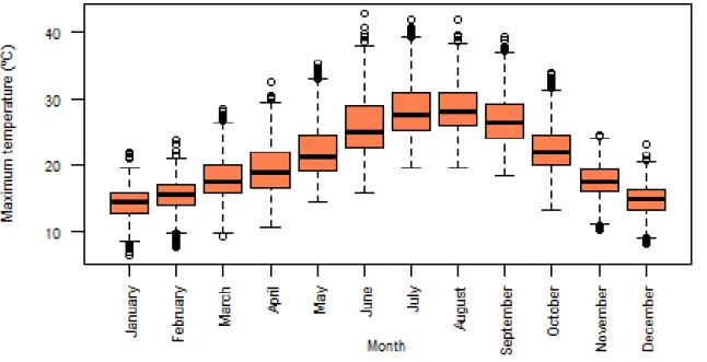
3.11 Boxplots of daily maximum temperatures by month. . . 27
3.12 Time series of daily maximum temperatures and total mortality. . . 27
3.13 Time series of daily maximum temperatures and total mortality of 2016. . . 28
3.14 Time series of daily maximum temperatures and total mortality of 1981. . . 29
3.15 Time Series of daily maximum temperatures and total mortality of 1991. . . 29
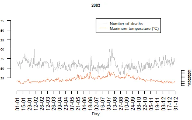
3.16 Time series of daily maximum temperatures and total mortality of 2003. . . 30
3.17 Time Series of daily maximum temperatures and total mortality of 2006. . . 30
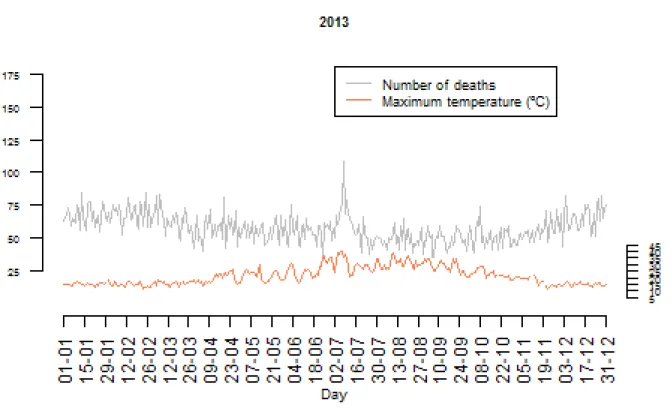
3.18 Time series of daily maximum temperatures and total mortality of 2013. . . 31
3.19 Time series of daily maximum temperatures and total mortality of 2017. . . 31
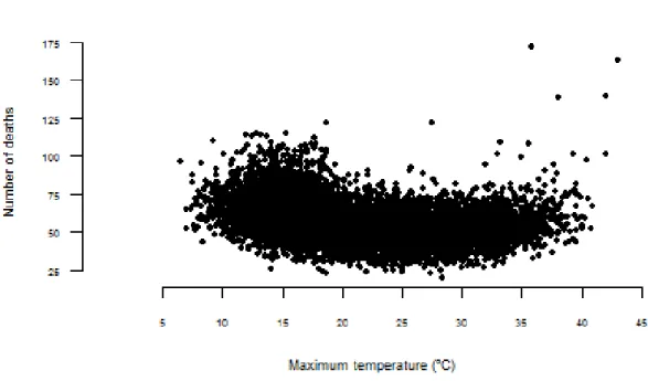
3.20 Scatter plot of the crude relationship of daily total mortality with daily maximum tem-perature. . . 32
3.21 Scatter plot of the crude relationship of daily total mortality with daily maximum tem-perature aggregated by mean. . . 32
3.22 Boxplots of daily mortality from May to September (total and stratified by age population). 33 3.23 Boxplots of total daily deaths by year, from May to September. And a regression line adjusted to the medians (green). . . 34
3.24 Boxplots of total daily deaths by month. . . 34
3.25 Boxplots of total daily deaths by day of the week, from May to September. . . 35
3.26 Boxplots of daily maximum temperatures by year, from May to September. And a re-gression line adjusted to the medians (green). . . 36
3.27 Boxplots of daily maximum temperatures by month. . . 36
3.28 Scatter plot of the crude relationship of daily total mortality with daily maximum tem-perature, using May to September data. . . 37
3.29 Scatter plot of the crude relationship of aggregated by mean daily total mortality with
daily maximum temperature, using May to September data. . . 37
3.30 Diagnostic plots of the final model. . . 42
3.31 3D plot of RR along temperature and lag. . . 43
3.32 Contour plot of RR along temperature and lag. . . 44
3.33 Plot of RR by the variable temperature (Var) at specific lags (left) and RR by lag at 0.1th, 90th, 95th and 99.9th percentiles of summer daily maximum temperatures distribution (right). . . 45
3.34 Plot of overall RR along temperature. . . 46
3.35 Plot of overall RR along temperature, predicted for years 1988 to 1997. . . 48
3.36 Plot of overall RR along temperature, predicted for years 1998 to 2007. . . 49
3.37 Plot of overall RR along temperature, predicted for years 2008 to 2017. . . 49
3.38 Boxplot of MAE obtained using 10 years length rolling-window evaluation vs. 5 years length rolling-window evaluation. . . 53
3.39 Boxplot of RMSE obtained using 10 years length rolling-window evaluation vs. 5 years length rolling-window evaluation. . . 53
3.40 Time series of the observed number of daily deaths vs. the predicted number of daily deaths by the ICARO model and the DLNM - year 1991. . . 54
3.41 Time series of the observed number of daily deaths vs. the predicted number of daily deaths by the ICARO model and the DLNM - year 2003. . . 55
3.42 Time series of the observed number of daily deaths vs. the predicted number of daily deaths by the ICARO model and the DLNM - year 2006. . . 55
3.43 Time series of the observed number of daily deaths vs. the predicted number of daily deaths by the ICARO model and the DLNM - year 2013. . . 56
3.44 Time series of the observed number of daily deaths vs. the predicted number of daily deaths by the ICARO model and the DLNM - year 2017. . . 56
List of Tables
3.1 Descriptive statistics of year-round data. . . 19 3.2 Descriptive statistics of only May to September data. . . 20 3.3 All basis-functions tested for the cross-basis (FunVar and FunLag), with respective
num-ber of degrees of freedom (df), numnum-ber of knots (nk) and the respective model quasi-AIC (QAIC). . . 39 3.4 Error Measures (MAE - mean absolute error; MSE - mean squared error; RMSE - root
mean squared error) obtained for each year tested using the rolling-origin update method of cross-validation. . . 47 3.5 Error Measures (MAE - mean absolute error; MSE - mean squared error; RMSE - root
mean squared error) obtained for each year tested using 10 years rolling-window evalu-ationmethod of cross-validation. . . 50 3.6 Error Measures (MAE - mean absolute error; MSE - mean squared error; RMSE - root
mean squared error) obtained for each year tested using 5 years rolling-window evalua-tionmethod of cross-validation. . . 51 3.7 Averaged Error Measures (MAE - mean absolute error; MSE - mean squared error;
RMSE - root mean squared error) obtained for all years tested by the 3 methods of cross-validation used, considering the ICARO model. . . 52 3.8 Averaged Error Measures (MAE - mean absolute error; MSE - mean squared error;
RMSE - root mean squared error) obtained for all years tested by the 3 methods of cross-validation used, considering the DLNM. . . 52
Chapter 1
Introduction
1.1
Background
1.1.1 The impact of weather on health
It is well known that temperature influences health and human comfort and it is currently accepted that mortality rates describe seasonal patterns, being higher in the winter and lower in the summer, with the exception of some rare peaks during summer that may be explained by the exposure to excessive heat [1, 2, 3]. So, one may say, temperature and death correlations are positive in summer and negative in winter [4], i.e., during summer, mortality increases because of very high temperatures, while during winter, it increases because of very low temperatures.
Also, the cold is known to provoke more adverse health effects in warmer countries and, contrariwise, heat is more dangerous in colder countries [5]. Thus it is perceived, there is no global optimal temper-ature for human comfort. Each population is adapted to its usual local climate [3], so the tempertemper-ature associated to better health and less mortality in each region is a determined percentile of temperatures felt in this location [6]. For this reason, this type of impacts must be studied locally, since temperatures that may have an adverse effect in one region, may have no effect at all in other regions, where people are adapted to those particular levels of cold or heat. More than that, the same population may adapt seasonally to different weather, becoming more tolerant to heat along summer and the inverse for winter [7].
Both extreme cold and extreme heat cause several adverse effects on human health:
On the one hand, cold has been associated with deaths in different countries, and some studies show that its impact is greater in poorer countries and countries with warmer winters [8], like Portugal which is one of the European countries with the highest excess winter mortality rate [1]. The exposition to low temperatures affects the human cardiovascular system, since it provokes vasoconstriction and increases blood pressure and cholesterol, which may cause heart attacks and strokes. At a respiratory level, cold may cause nose congestion, rhinorrhea and bronchoconstriction and exacerbate preexisting conditions of people who suffer from asthma or chronic obstructive pulmonary disease, leading to death in the worst case scenarios [5].
On the other hand, heat is also responsible for a large number of hospitalisations every year [9], once it can cause several malaise, like severe dehydration, exhaustion, cramps, oedema, heatstroke, acute cerebrovascular accidents ant it is responsible for the aggravation of preexisting illnesses, as pulmonary chronic diseases, cardiac conditions and kidney disorders [10]. Unfortunately, many of such problems may evolve to death, a risk which is higher for people who have some of the identified risk factors:
cog-nitive limitations, isolation, low socioeconomic status, advanced age and living in urban areas, among many other [7, 9]. Although, the older individuals suffer more with heat adverse effects, there are reg-istries of severe heatwaves with some impacts on all group ages mortalities [7].
This work was intended to focus on the effects of heat on mortality rates, even though mortality is higher during the cold months; because its correlation with heat is stronger [4] and also because the global average temperatures are increasing due to climate changes. Hence, it is important to study phenomena like heatwaves with impact on health, even though it has no consensual definition on the literature [3, 9]. From a strictly meteorological point of view, the World Meteorological Organization has defined a heatwave as a period of at least six consecutive days with maximum temperatures 5 oC above the average daily temperatures for the respective time period [11]. However, this definition is not directly related to the heat impacts on human health. From a public health point of view, a heatwave is usually described as several consecutive days above a determined air temperature threshold, but the number of days to be considered is not clear and the temperature threshold changes for different regions and populations [7]. Therefore, in this work the term “heat wave” will be used to refer to a period of excess heat that impacts human mortality.
Nevertheless, extreme heat is associated with an increase in mortality [3, 7] and morbidity, which impacts health care systems, being considered a public health problem for those reasons [7]. It is impor-tant to note that heat related deaths could be decreased with a suitable warning and response system to heat emergencies [9].
In Portugal, several heatwaves and their impacts in mortality have been registered since the final decades of last century [7, 12, 13]:
• June 1981 - excess mortality estimated in 1900 deaths • July 1991 - excess mortality estimated in 1000 deaths
• July/August 2003 - excess mortality estimated in 2000 deaths • July 2006 - excess mortality estimated in 1100 deaths
• June/July 2013 - excess mortality estimated in 1700 deaths
Due to climate change, both minimum and maximum temperatures are increasing [1]. Besides, most scientists expect extreme weather phenomena, like heat and coldwaves, with sudden drops or increases in temperature, to happen more intense and frequently in the next few decades [1, 9, 10, 14]. These facts, together with ageing and ever more urbanised Portuguese population (two risk factors for heat vulnerability [7, 9]), suggest strongly that summer mortality will increase in the coming years, eventually becoming an urgent public health problem. As such, temperature-mortality relation must be deeply studied, in order to predict the consequences of global warming, particularly for those most vulnerable and least able to adapt [9].
1.1.2 The ICARO surveillance system
In Portugal, the heatwaves of 1981 and 1991 were responsible for a very high number of deaths in a short time, as described previously. As those deaths were clearly related to an excessive heat, it is safe to say that at least part of them would have been avoidable [12], showing that extreme heat is an important health problem in the country [15]. Hereupon, there was a need to create a heat surveillance and warning
1.1 Background
system, in order to mitigate this effect, which led to the ICARO surveillance system being implemented in 1999 [7, 12, 15].
ICARO is an acronym for Importˆancia do CAlor: Repercuss˜ao sobre os ´Obitos, which means Im-portance of Heat and its Repercussions in Deaths[15]. It is a heat health warning system that monitors possible increases in mortality due to extreme heat and is set in motion every year between May and September [7, 12]. It was constructed by the portuguese national health institute (INSA) - that developed statistical models in order to understand how weather variables relate to heat associated mortality -, in a partnership with the portuguese meteorology institute (IPMA) that provides registries and three-day predictions of temperatures [12].
INSA initially developed a time series statistical model using dynamic regression techniques, which were calibrated for Lisbon data concerning the 1981 and 1991 heatwaves [12, 15] and it was later updated to account for the prolonged heatwave of 2003 with the implementation of a dynamic threshold [7].
In this work, the model that will be considered as the ICARO model is the model for the district of Lisbon, proposed by Nogueira & Paix˜ao [7], which will be refered to as ICARO Lisbon. It takes as independent variable the generalised accumulated thermal overload (GATO) - a combination of two weather direct functions [7]:
1. GHLen - a generalised function of the heatwave length, that counts the number of consecutive days in which the maximum temperature went above the considered threshold. This function was constructed in such way that keeps considering the effect of several days with excessive heat even if the temperature lowers under the defined threshold for a few days in between [7].
2. Exc - corresponds to the observed excess temperature above the considered threshold [2, 7]. The threshold used - τ - is a dynamic threshold that depends on the week, beginning as τ = 29oC in May and then increasing 1oC every week since week 22 (end of May/ beginning of June) until week 28 (second week of July), remaining τ = 35oC until the end of September [7]:
τw(t)= 29 + (w(t) − 22) , if week 22 ≤ w(t) < week 28 35 , if w(t) ≥ week 28 , (1.1)
with w(t) = isoweek of the day t.
Then, τw(t) enters the two weather direct functions, considering the daily maximum temperatures
(MaxTt):
Number of consecutive days above the threshold τw(t):
GHLent = GHLent−1+ 1 , if MaxTt ≥ τw(t)
GHLent−1− 1 , if MaxTt < τw(t) & GHLent−1> 0
0 , if MaxTt < τw(t) & GHLent−1= 0
(1.2)
Excess temperature above the threshold τw(t):
Exct = MaxTt− τw(t) , if MaxTt≥ τw(t) 0 , if MaxTt≤ τw(t) (1.3) Neither GHLent and Exct, if considered on their own, are highly related with mortality, but their
daily mortality [2, 7]:
GAT Ot = GHLent× Exct (1.4)
GAT Oenters the model so to predict the expected daily mortality taking into account the high tem-peratures effect [2, 7, 12]. The generic model tested for the ICARO Lisbon is a regression linear model following:
Yt = C + α ×Year + β × GAT Ot−1+ γ × GAT Ot+ δ × Exct+ εt , (1.5)
where
• Yt is the number of deaths in day t;
• C is the regression constant; • Year is a linear term of the year;
• α, β , γ and δ are regression parameters; • εt is a random process.
This model is based on the observed and predicted temperatures for 3 days (given by IPMA) [7, 15] and showed to be well adjusted to the data, to easily detect the extreme heat impacts on mortality. However, it overestimates some of the mortality increases [2, 12] and, on the other hand, it seems to underestimate the later observed impacts of a long heatwave [7].
Even so, the estimate daily mortality with heat effect is then used to calculate the ICARO Index (II) [12]:
II= Number of expected deaths with heat effect
Number of expected deaths without heat effect− 1 (1.6) The II gives the excess relative risk of deaths due to heat effect and will be zero if there is no expected effect [12].
Nowadays, there is in place a system with mainland Portugal coverage, which uses a generic model similar to the one described. However it considers predefined thresholds, instead of dynamic ones, like the Lisbon model does. Everyday between May and September, a daily report - the ICARO Index Report - is built and sent to the Portuguese National Health Directorate and the Portuguese National Service of Fireman and Civil Protection, among others [12]. The report presents:
• the 48 most recent predictions of the II (which includes the adjusted value for the previous day and the values for the current day and the 2 following days), with information about the statistical significance of the predictions;
• the highest II registered, as a comparison term;
• the predicted maximum and minimum temperatures for the 2 following days in the 18 districts of mainland Portugal;
1.2 Objectives
1.2
Objectives
As mentioned before, the model used on ICARO Lisbon overestimates the mortality increases caused by heatwaves [2, 12] and tends to underestimate their later impact [7]. For that reason, we propose to formulate a new statistical model with equal sensitivity but better specificity, i.e., a model that keeps ICARO’s good capacity to detect heatwaves with expected impact on mortality, but that also accounts for later impacts and prevent false alarms, which may discredit future warnings. To formulate such a new model we have tried to take into account the different features of the heat-mortality relationship, described in the literature:
• Non-linear relation - various studies investigated the relation between temperature and mortality and showed that it is U-, V- or J-shaped, with mortality increasing for extremely low or high temperatures [7, 14, 16, 17, 18, 19, 20]. These shapes indicate a non-linear heat-mortality relation, as already described in the literature [4, 7, 16, 17].
• No immediate effect - it has also been reported that the effect of extreme heat is sustained in time [3, 14, 16, 21], so the rise in mortality does not just occur immediately when the temperature increases, but has been described to last 1 to 5 days after the excessive heat day [7, 9, 14, 22]. • Harvesting effect - there is evidence that heat causes the death of people who are in poor health
conditions and who would probably die otherwise a few days or weeks later, even without the high temperatures [9, 16]. In other words, heat may just anticipate unavoidable deaths, a phenomenon called harvesting, which increases the complexity of modelling the heat-death effect [21].
• Isolated and sustained heat effect - there are commonly two different ways for approaching the effects of heat on health: one is to take warm days as single episodes, considering isolated daily temperatures; the other is to consider temperature as a continuous risk factor, taking into account series of daily temperatures [3]. Both can be combined, describing the mortality risk to increase due to the independent effect of isolated days with high temperatures and also with the duration of consecutive days with high temperatures - sustained effect [3, 16].
That being said, we propose to consider a model capable of combining non-linear exposure-response functions (in this case, temperature-mortality) with non-linear distribution of the time - lags - effect in order to account for the different weight of each past days’ temperatures effect in the mortality of the present day. For that reason, the main goal of this work is to develop a distributed lag non-linear model (DLNM) to monitor the mortality increases caused by heat. This model will include a time dimension in order to better predict the delayed effect of heat in mortality, as well as its cumulative effect. It will be used to study the extreme heat effects on Lisbon’s mortality, aiming to optimise/update the model used in the ICARO system.
1.3
Work Structure
This Masters dissertation consists of 4 chapters: Introduction, Materials and Methods, Results and Discussion.
The first and present chapter presents the background of the research’s theme. The adverse effects of heat on human health and mortality are explained as well as how the ICARO surveillance and alert system works. Lastly, the goals of the research are enunciated.
Chapter two presents all the data accessed and its transformations. Besides, the statistical methods that will be used to model the daily mortality in the district of Lisbon as a function of daily temperatures will be referenced and it will be explained what is a distributed lag non-linear model. Moreover, the method used to compare the new model obtained (DLNM) with the model currently used by the ICARO system - cross validation - will be presented.
The third chapter presents the results of the exploratory data analysis of the variables that will enter the proposed model. The chapter also shows the results of the adjustment of the new model (DLNM) and the results of the assessment and comparison of DLNM against the ICARO model, as well as the analysis of these results.
Finally, chapter four consists of the discussion and conclusions of this work, considering its limita-tions, as well as possible future developments of this theme.
Chapter 2
Materials and Methods
2.1
Data Collection
In this work, it was decided to study the heat-mortality relation for the district of Lisbon.
For this purpose, we accessed Lisbon’s daily total death toll numbers between 1980 and 2017 and stratified these deaths (by all causes) into two age groups: population under and 65 years of age and above. All this data was provided by the Statistics Portugal (INE).
The weather data was provided by the Portuguese Institute for Sea and Atmosphere (IPMA) and consists of the Gago Coutinho meteorological station daily records of minimum and maximum air tem-perature in Celsius degrees for the period between 1980 and 2018. Yet, it was decided to use only the data until year 2017 since the counts of deaths for 2018 were not available.
INE also provided the average annual resident total population in Lisbon’s district for the years between 1980 and 2017 and the data concerning the district’s over 65 years old population between 1992 and 2017. The total resident population will be used to control for possible confounding.
2.1.1 New Variables
The collected weather data was used to create some more variables that, according to the literature, might relate with mortality. Namely, the daily thermal amplitude, calculated as the difference between the maximum and minimum air temperatures for each day, and an approximation to the daily mean temperature, calculated as the average of the minimum and maximum air temperatures [14].
Also, the average resident population under 65 years of age for the years between 1992 and 2017 was calculated as the difference between the total population number and the number of the population aged 65 and above.
This way, there are a total of 10 variables (all referring to the district of Lisbon) that can be used in the statistical analysis:
• Daily counts of total number of deaths (TMort)
• Daily counts of number of deaths of people with 65 years old or more (≥ 65Mort) • Daily counts of number of deaths of people under 65 years old (< 65Mort) • Daily maximum temperature (MaxT)
• Daily mean temperature (MeanT) • Daily thermal amplitude (TA)
• Annual average of the total resident population (TPop)
• Annual average of the 65 years old or more resident population (≥ 65Pop) • Annual average of the under 65 years old resident population (< 65Pop)
From these ten variables, the data that will enter the modelling is: the daily counts of total number of deaths, the daily maximum temperatures and the annual average of the total resident population. The rest of the collected data will only be taken into account in the exploratory analysis, in order to provide a broader picture of the whole Lisbon’s mortality-temperature-population scenario.
2.2 Statistical Methods
2.2
Statistical Methods
In this work all the statistical analysis will be undertaken in several different R 3.5.2 software packages. R is a free software environment for statistical computing and graphics (http://www. r-project.org) [23]. In particular, the dlnm package, developed by Gasparrini (2015) [24], will be used, as it offers some functions to run DLNMs in a simple way.
2.2.1 Exploratory data analysis
In order to become more familiar with the data set, statistical analysis should always start with an exploratory data analysis. Exploratory data analysis consists of collecting basic descriptive statistics of the variables and visualising the data trough simple exploratory graphs.
The descriptive statistics will be obtained using the R functions summary() and sd() from the package stats. The first one gives measures of location and number of missing values and the second one gives a measure of dispersion or variability - the standard deviation.
The initial exploratory analysis will also employ time series graphs, i.e., graphic representations of repeated measurements taken over regular time intervals (daily counts of deaths and temperatures, and yearly population densities, in what concerns this thesis), as well as boxplots. Both aim to facilitate the perception of the numeric variability, trend and seasonality of the different variables. Moreover, correlation graphs of daily mortalities vs. daily temperatures will be presented.
2.2.2 Distributed lag non-linear models
Oftentimes, the effect of exposure to environmental stressors or other events is not limited to the time period when it occurs, but is delayed in time [21]. That is the case of climatic variables effects (as adverse temperatures) that may last in time, spreading over several days [8, 17, 21, 25], as mentioned in the introduction chapter. That being said, the impact of the environmental stressors at a given time may be explained by a combination of past exposures over several time lags [21], once it depends simultaneously on the intensity and timing of the exposures [26]. A common way to model a non-linear effect with this additional time dimension is through distributed lag non-linear models (DLNMs) [1, 6, 9, 14, 17, 27].
The family of distributed lag linear models was developed to simultaneously estimate the non-linear dose-response dependencies and the delayed effects of temperature on mortality [21]. It is based on a bidimensional space of functions, called “cross-basis”, that describes the shape of the relationship simultaneously along the space of the predictor - temperature, in this case - and along its lag dimension, i.e., the time structure of the exposure–response relationship [21]. This way, each exposure up to a maximum lag may be summed to obtain the cumulative effect of temperature [17].
Initially, distributed lag models (DLMs) were developed for time series analysis and extensively used in econometric and social sciences before being adapted to epidemiology research [28, 29]. This family of models used to account for linear dependencies only, so Armstrong [16] extended this methodology to distributed lag non-linear models (DLNMs), and it has since been used to simultaneously estimate the non-linear and delayed effects of temperature and air pollution on mortality or morbidity [1, 16, 17, 21, 26, 29]. Hence, to understand a DLNM well one must first understand DLMs.
time moments t. It can generally be represented as follows: yt= α + β0xt+ β1xt−1+ ... + βlxt−l+ ... + βLxt−L+ ut = α + L
∑
l=0 βlxt−l+ ut , (2.1)where α is the intercept, ut is a stationary error term and L is the maximum lag allowed (L ≥ 1) [30].
Each of the coefficients βlstands for the weight of the respective lag l (l = 0, 1, ..., L). βl coefficients
may be interpreted either from a backward standpoint - the effect of the past exposition xt−l on the
present moment response yt, i.e., the effect felt today due to the exposition l days before, lag = l -, or
from a forward standpoint - the effect of the current exposition xt on the future response l moments later,
yt+l, i.e., the effect that today’s exposure will cause l days from now [26, 31]. Thus, the coefficients βl
represent the lag weights and all together define the lag distribution [30].
Assuming there is a temporary change on the regressor variable x, which increases one unit only in moment t (xt), then its immediate effect, yt, will have an increase equal to the value of β0. On the next
moment (t+1) the effect yt+1will increase β1units. After that the effect yt+2will increase β2units and so
on, until the maximum lag, L, when the effect yt+Lincreases βLunits. This is called the marginal effect
of x on y.
Another hypothesis to consider would be a permanent change in the regressor variable. Assuming it increases one unit in moment t and remains that high in all future moments, then its immediate effect yt will also have an increase equal to the value of β0. However, in the future moment (t+1) the effect
yt+1will increase β0+ β1values, after which the effect yt+2will increase β0+ β1+ β2values and so on,
until the maximum lag L, when the effect yt+Lincreases β0+ β1+ β2+ ... + βLvalues. This is called the
cumulative effect of x on y [30].
Variable x may change more or less than one unit and increase or decrease. These changes may occur at any moment, be temporary or permanent. Therefore, from (2.1), we understand that the change on yt
depends on the sum of the products of each past moment value of xt−land the weight of its moment βl,
with 0 ≤ l ≤ L. As such, the combination of all lag weights (the cumulative and marginal effects) defines the pattern of how the magnitude and timing of x influences y over time.
In this modelling approach that includes one parameter βl to each lag, each individual coefficient is
highly correlated to the others, which raises a problem of collinearity. That problem, however, has been overcome with the imposition of some restrictions to βl, originating a constrained distributed lag model
[16, 21]. According to Armstrong (2006) [16], the constraints may consist in compelling the coefficients βl to be equal for a determined range of lags - which is called a lag-stratified distributed lag model - or
in forcing βl to follow some smooth curves, as a polynomial, a natural cubic spline or a penalised spline
function, among other options.
For now, we will focus only on the relation of the regressor x and the response y, defined as s(x,t). According to Gasparrini (2014) [26] and assuming there is a linear exposure–response relationship, a general notation to describe the dependency in terms of exposure history to x evaluated at time t is:
s(x,t) = Z L l0 xt−lw(l) dl ≈ L
∑
xt−lw(l) , (2.2)2.2 Statistical Methods
where w(l) represents the weighting basis-function applied to constrain the coefficients βl. w(l) is
di-rectly defined in the lag dimension and determines the lag-response function that models the lag–response curve associated with exposure x, [26].
s(x,t) will then be included in a generalised linear model as a sum of linear terms, with related parameters η.
The function s(x,t), defined in (2.2), may be rewritten following a matrix notation, by applying the basis transformation over the lags - w(l) - and then combining it with the vector of expositions qt[21, 26]:
s(xt; η) = qtCη = W T
t η , (2.3)
where
• qt = [xt, ..., xt−l, ..., xt−L]T is an original vector of ordered exposure histories, corresponding to a
column of the n × (L + 1) matrix Q [21]. As such qtchanges along time, depending on the moment
twhen it is defined [26];
• l = [0, ..., l, ..., L]T is a vector of lags corresponding to the L+1 columns of Q [21];
• C is a (L+1)×υlmatrix of lag-basis variables originated from the application of the basis-function
to the lag vector l (where the basis-function is defined as w(l) with dimension υl);
• η is a vector of unknown parameters.
Hereupon, WTt is a vector from the matrix W = QC, which is the matrix of the υl transformed
variables (obtained from the application of a basis lag function to the original lag vectors l w(l) -combined with the original exposure histories, qt). This υl basis variables from the matrix W will be
included in the design matrix to allow the estimation of the unknown parameters η. The estimated parameters ˆη define the previously mentioned coefficients βl [21]:
ˆ
β = C ˆη (2.4)
The extension from DLM to distributed lag non-linear models (DLNM) was achieved by adding an exposure–response non-linear function along the dimension of the predictor x [26]:
s(xt; β ) = ZTt.β (2.5)
On this function, ZtT.is the tthline of the matrix Z - a n × υxbasis matrix resulting from the application
of the basis-function - called f (x), of dimension υx-, to the original vector of exposures x [21].
Therefore, a generalisation of (2.2) to DLNM will be adding a basis-function along the dimension of the predictor x to the already mentioned basis-function along the dimension of the lag l:
s(x,t) = Z L l0 f(xt−l) w(l) dl ≈ L
∑
l=l0 f(xt−l) w(l) , (2.6)where f (x) is the exposure-response function with dimension υx and w(l) is the previously mentioned
other [16, 26]. The basis-functions impose a set of completely known transformations of x, generating new variables, called basis variables [21].
The representation in (2.6) assumes that the functions f (x) and w(l) are independent, i.e., that the exposure-response function is the same along all the lag space and that the lag structure is equal for all values of x [26]. If we relax this assumption, admitting an interaction between the value of the predictor and its timing, then (2.6) may be more flexibly represented as:
s(x,t) = Z L l0 f· w(xt−l, l) dl = L
∑
l=l0 f· w(xt−l, l) (2.7)Following this notation, f · w(x, l) is a bivariate function, that models simultaneously the exposure-response structure along x and the the lag-exposure-response structure along l, defining the exposure–lag–exposure-response function[26]. In other words, s(x,t) is a linear combination of the basis-functions f (x) and w(l), inte-grated over the lag dimension, which defines a bidimensional space of functions that Armstrong (2006) [16] called cross-basis function and which represent the core of DLNMs [16, 26, 32].
Each basis-function ( f (x) = ∑Bb=1βbxband w(l) = ∑Pp=1βplp) is fitted following the chosen function
distribution, f () and w() respectively, originating B/P basis variables from the original ones. Then the new transformed variables will enter the regression model, instead of the original variables. The number of basis variables, B and P, determines the degrees of freedom (df) of the respective curves [16]. B df for the dimension of the predictor and P df for the dimension of the lags. So the degrees of freedom of the cross basis-function is given by the product of the number of basis variables from f (x) and from w(l), B× P.
The cross-basis function is better represented using matrix notation as Gasparrini et al. [21].
Let ˙Rbe a n × υx× (L + 1) array of the lagged occurrences of each of the basis variables of x, keeping
C as the matrix of basis variables for the lag dimension,
s(xt; η) = υx
∑
j=1 υl∑
k=1 rTt jc.kηjk= wTt η , (2.8)where rt j is the vector of lagged exposures for the time t transformed through the basis-function j and
c.kis the vector of lags transformed trough the basis-function k.
Now, wTt will be defined as the vector obtained by applying the υx· υlcross-basis functions to xt. As
such, both basis-functions are then simultaneously used to create the υx× υl basis variables, stored in
the W matrix.
According to Gasparrini et al. [21], in order to reach a compact formula for W, there is a need to represent it as a tensor product, ˙A, defined as a n × (υx· υl) × (L + 1) array, that will be rearranged
summing along the third dimension of lags, obtaining W, the final matrix of the cross-basis variables values and η, the associated parameters, expressed in (2.8) [26].
In conclusion, the cross-basis flexibly describes the relation along x, allowing for linear and non-linear exposure-responses, combining it with the distributed lag-effects (an additional time-dimension) [26]. So, the υx× υl basis variables originated from the cross-basis function will enter the regression
model instead of the original variables.
2.2 Statistical Methods
defined in (2.8), to express the non-linear relation between the predictor variable x and the response variable y along time. Following the notation of Gasparrini et al. [21], we obtain:
g(µt) = α + J
∑
j=1 sj(xt j; ηj) + K∑
k=1 γkutk , (2.9)where µt ≡ E(Yt) and g is a monotonic link function; α is the intercept; sj is the cross-basis function
that denotes smoothed relationships between the variables xj and the linear predictor - defined by the
parameter vectors ηj -, and uk are other predictors variables with linear effects over Y, measured by the
coefficients γk.
This type of functions (DLNM) should be more adequate for this kind of modelling than simpler ones, because they reduce the risk of confounding by a residual main effect of heat on consecutive days [3].
In this family of models, Y is assumed to follow a distribution from the exponential family [21]. The two basis-functions used in the cross-basis sj may be chosen from a wide variety of modelling options
[16, 21, 26]. Armstrong (2006) [16] has reviewed the options suitable to model the relationship between ambient temperature and daily mortality. Those options are:
• for the shape of the temperature–mortality curve at a given lag: – a polynomial function, whose order must be determined; – a stratified model, with chosen strata intervals;
– a spline function, for which the number and placing of knots must be chosen; – linear thresholds;
• for the change in coefficients by lag:
– a polynomial function, whose order must be determined; – a stratified model, with chosen strata intervals;
– a spline function, for which the number and placing of knots must be chosen; – the coefficients may be unconstrained;
The options selected will determine the flexibility of the model. Simpler models (as linear thresholds) are usually less flexible but easier to interpret than the more complex ones (as natural cubic splines functions), while the latter may better adjust to the data and capture most of the relationship details and are less likely to leave residual confounding [16].
Other predictor variables may be included in the model. For instance, as happens in order to control for confounding, a smooth function of time to capture long-time trends and/or seasonality and some categorical variables, as day of the week [21], are applied.
Also, the analysts must determine the maximum lag, L, which will depend on how long they believe an effect may be sustained in time. For instance, the maximum lag allowed should be higher if harvesting effects are expected, which may reflect on negative coefficients for longer lags [16],.
All options have advantages and disadvantages, so the choice will depend on the purpose of the analysis, on a priori assumptions and/or the fitting of the model. The model fitting criteria mostly used in this context are the modified Akaike’s information criteria (QAIC) and the modified Bayesian
information criteria (QBIC) for models with overdispersed responses fitted through quasi-likelihood [21], with the following expressions:
QAIC= −2L ( ˆθ) + 2 ˆφk (2.10)
and
QBIC= −2L ( ˆθ) + log(n) ˆφk , (2.11)
whereL is the log-likelihood of the fitted model with parameters ˆθ; ˆφ is the estimated overdispersion parameter; k is the number of parameters and n is the number of observations.
These two information criteria are goodness-of-fit measures that evaluate the quality of the models. They equally assess the sum of squared residuals through the log-likelihood function, but penalise dif-ferently large numbers of estimated parameters [30]. As both criteria estimate the amount of information lost by a model, it is aimed to minimise them. The model with the lowest QAIC or QBIC should be the one which lost less information, i.e., should be the higher quality model.
Previous studies found that the QAIC provides better results than the QBIC in this context [16, 26]. Therefore, along with other previous approaches, we will only consider the QAIC in this work [1, 19, 31]. 2.2.2.1 Heat-mortality modelling
The purpose of this work is to model the impact of heat on mortality in the district of Lisbon, so the main focus, data wise, are days with excessive heat and heatwaves, that usually occur during or around summer. For that reason, the modelling will be restricted to the months from May to September, as in the current model used by the ICARO system [12]. This way, the time series model becomes simpler, with less auto-correlated errors [7]. From now on, this five months period will be generally referred to as the “summer period”.
The data available spans from January 1st of 1980 to December 31st of 2017, so there will be a total
of 38 years. Since this work will focus only in the summer period, the data to be used is assumed to come from several time series, each one corresponding to the period between May and September of each year, i.e., 38 groups/sections from the original complete time series.
The impact of heat on mortality will be studied considering a maximum lag of 10 days, as the literature shows that 10 days are enough to capture the delayed and harvesting effects of heat [3, 33]. Thus, to assess the effect that the 10 previous days have on the first day of May, we must account for the last 10 days of April. This way, there will be a total of 6194 observations, each one corresponding to a day between April 21stand September 30thfrom the years 1980 to 2017.
The model employed will be a DLNM that follows (2.9). The response variable, Yt, will be daily
counts of deaths, which is assumed to arise from an overdispersed Poisson distribution with a canonical log-link function: E(Y ) = µ and V (Y ) = θ µ, where θ is the dispersion parameter.
As mentioned in section 2.1, the average annual total resident population in Lisbon is available for the all period between 1980 and 2017. However, resident population data stratified by age is only available from 1992. For that reason, it was decided that the total daily counts of deaths would be used as the response variable in the model (instead of counts of deaths stratified by age) to better control for this possible confounding of resident population during a larger time period.
The predictor variable, Xt, will be maximum daily temperature, once it is intended to study how
extreme heat affects mortality rates and to better compare the results with the current ICARO model, which uses maximum temperatures.
2.2 Statistical Methods
The main focus of this type of models (DLNMs) is the cross-basis function, for which we must choose two functions: one to the exposure-response curve and another to the lag-response curve. As pre-viously mentioned, there is a large amount of options for these two functions. Hence, we will construct several models using natural cubic B-splines (ns) and quadratic B-splines (bs) as the basis-functions, which are the type of functions more frequently mentioned in the literature for modelling the effects of extreme temperatures on mortality [3, 6, 14, 17, 19, 21, 27, 32].
It must be noted that the larger number of knots chosen, larger the number of df, the more flexible but less smooth will the shape of the function be [17, 21]. Therefore, the choice of number of knots, which determines the smoothness of the curve, is more important than precise knot placement, with many knots tending to show spurious wiggles and too few knots losing real wiggles [16]. For this reason, we will try different number of knots (3 to 5) for both basis variables, allowing them to be equally spaced with no intercept, following the chosen spline function for the predictor dimension, and equally spaced in the log scale with an intercept in the lag dimension.
The QAIC will be used to chose each basis-function’s most appropriate degree of the spline (quadratic or cubic) and the number of knots (3 to 5), which determines the degrees of freedom:
• Natural cubic B-spline: Number of knots = df - 1 - intercept • Quadratic B-spline: Number of knots = df - 2 - intercept
Regression diagnostics such as residual plots are also presented, as they may be helpful in the selec-tion of different models [21].
To control for seasonality, a natural cubic B-spline of day of the season with 4 internal knots, defining 5 degrees of freedom (one for each month - May to September) will be used. In its term, the long-term trend will be controlled for with a natural cubic B-spline of time with 3 internal knots, defining 4 degrees of freedom (approximately one for each decade). Moreover, the model will include day of the week as a categorical variable and population as a linear variable (entering he model as an offset). All these decisions were based on previous work restricted to one season [1, 33].
The selected model will then be used to predict the relative risk (RR) associated to determined com-binations of temperature and lag values vs. a reference temperature associated to the minimum mortality. As effects on health are more associated with temperature percentiles than absolute temperature [6], which is due to climate adaptation, we chose as minimum mortality temperature the 75thpercentile of the yearly maximum temperatures registered in Lisbon for the period in analysis (1980-2017), which is 25.7oC. This methodological option is consistent with previously published work [3, 6].
2.2.3 Models assessment and comparison
Finally, the chosen DLNM will be compared with the model considered for Lisbon in the ICARO system. Given that the statistical model used by ICARO is a linear regression model which does not account for overdispersion, it does not make sense to calculate its QAIC, so this criteria cannot be used for comparison with our DLNM. Hence, another method to evaluate both models and allow a fair comparison between them is needed. As both models will be used to forecast future response values (number of daily deaths), one common method to assess and compare them is to evaluate their predictive performances. The model that better predicts future response variables will be considered the best model. This may be achieved through cross-validation.
Cross-validation is a common technique to estimate how accurately a predictive model will perform on new (unseen) data. It consists in splitting the data set in two complementary groups. One subset is
called training data and will be used to perform the analysis, adjusting the estimates parameters of the model. The other subset, called test data, will be used to validate the analysis, making predictions for this new data subset and obtaining some measures of fitness to estimate the predictive performance of the model. This process allows to detect problems such as overfitting or bias, once the forecast will be made in data that had not been taken into account during the adjustment of the model. There is a broad range of data partitioning methods and usually multiple rounds of cross-validation are performed with different partitions of the data set in each round, to reduce variability.
Given that we are working with time series, it is important to be particularly careful when choosing the partitioning method. Most partitioning methods are random processes that split the data into two subsets without keeping the order of the observations. However, in time series analysis the observations follow a specific sequence and may not be considered as independent. For that reason, the most common approach of cross-validation for time series analysis is the last block evaluation [34]. It consists of continuous forecasting of upcoming values, where the origin of the test data follows the last known value of the train data. This way the dependencies of the data are respected, assuming that the future (that which we want to predict) depends on the past (which we used for modelling) [34]. Once again, there is more than one method for partitioning the data for last block evaluation. Following Bergmeir’s (2012) nomenclature [34], this research work will perform two different partitions, the rolling-origin-update and the rolling-window evaluation.
In order to perform the rolling-origin-update, we will start by adjusting the models to data corre-sponding to the first 10 years of our complete data set (1980 to 1989) - train data - and then evaluate their predictive performance to the subsequent year (1990) - test data. The process will then be repeated, including the previous test data in our training data (which will now be from 1980 to 1990) and readjust-ing the model for the new trainreadjust-ing data as well as to test it on the new test data (1991) and so on. This process will occur time and again, until the “final round”, when the training data will be from 1980 to 2016 and the test data will correspond to the year of 2017.
As a result, predictions of daily deaths to all summer periods from the year 1990 to 2017 will be obtained by the two models (DLNM and ICARO). The predictions obtained for each year will be based on the models adjusted by all the previous years’ data (since 1980). This method simulates real-life application, once it used all past information available to predict each upcoming summer heat-related mortality and then the data from each new year integrates the data set used for adjusting the model, which will again be used for forecasting the new summer period and so on, repeating the whole process every year.
As the training data grows bigger, this proceeding may have the disadvantage of old values disturbing the present model forecast. This possibility is quite strong in this scenario because population changes along the years, and it is likely to be more protected from heat in the present moment, due to better adap-tation habits and socioeconomic as well as housing conditions, among other factors that may decrease the adverse effect of heat. Therefore, the relationship between adverse temperature and deaths in 2019 is not the same as it was in 1980. Hereupon, it may be wise to consider a fix length window for the training data.
Following this rational, plots of the overall RR along temperatures estimated by the DLNM adjusted for different time periods (1980-1989; 1990-1999; 2000-2009 and 2010-2017) will be present. Those will show if there were any evolution of the heat-mortality relationship along time. If so, it makes sense to also consider rolling window evaluation.
To perform rolling window evaluations, the first step is to choose the length of the window, i.e., the dimension of the time period considered to adjust the models. Lets consider a train data length of 10
2.2 Statistical Methods
years. In this case, as in the rolling-origin-update approach, we would start by adjusting the models to data corresponding to the first 10 years of our data set (1980 to 1989) - train data - and then we would evaluate their predictive performance to the subsequent year (1990) - test data -. Then we would repeat the process, but now moving the all window forward one year. The test data will enter our training data, which will lose the first year. Now the new train data would become from 1981 to 1990. Then we readjust the model for the new training data and test it on the new test data (1991). And so on, keeping always a train data with 10 years, until the final round, when the training data will be from 2007 to 2016 and the test data will correspond to the year 2017. As a result we will also obtain the two models (DLM and ICARO) predictions of daily deaths to all summer periods from the year 1990 to 2017, but now the predictions obtained for each year will be based on the models adjusted only by the data of the 10 previous years.
This procedure will be repeated using different lengths for the window, to check if the estimated effect of heat on mortality changes with different number of years entering the modelling. We will empirically use 10 and 5 years windows.
As a result of each round from both methods, error measures will be obtained to evaluate the predic-tive performance of both ICARO and DLNM models. An error is the difference between an observed response value on moment t (yt) and the value predicted by the model for this same moment ( ˆyt). So the
absolute error (AE) is given by |yt− ˆyt| and the squared errors (SE) is given by (yt− ˆyt)2. Then the errors
in each round are averaged for an easier interpretation.
The error measures used in this work are the mean of the absolute errors (MAE), the mean of the squared errors (MSE) and the root of the mean squared errors (RMSE), obtained by the following ex-pressions: MAE =1 n n
∑
t=1 |yt− ˆyt| (2.12) MSE= 1 n n∑
t=1 (yt− ˆyt)2 (2.13) RMSE= s 1 n n∑
t=1 (yt− ˆyt)2 (2.14)The comparison of the two models will be based on these error measures. The model with the lowest error measures is the one whose predictions for the unseen data are closer to the real observed values, which means that it is the model that better generalised to new data. In summary, the lowest error measures, the better is the predictive performance of the model.
This comparison will also allow to choose how many years should be accounted in the estimation of the models parameters to allow a better prediction of the upcoming summer. The cross-validation method with lower error measures, is the one with the best training data choice.
Also, to better understand the different performances of the ICARO and the distributed lag non-linear models (using the best train data length for each model, chosen by the cross-validation), there will be constructed some time series graphs of the observed daily deaths and the respective predicted number of daily deaths by each of the models (ICARO and DLNM) for the years tested with known heatwaves (1991, 2003, 2006, 2013 and 2017). This will allow an easy interpretation of the performing differences between the two models.
Chapter 3
Results
3.1
Exploratory Data Analysis
In this section, the results of the exploratory data analysis described in section 2.2.1 are presented. 3.1.1 Descriptive statistics
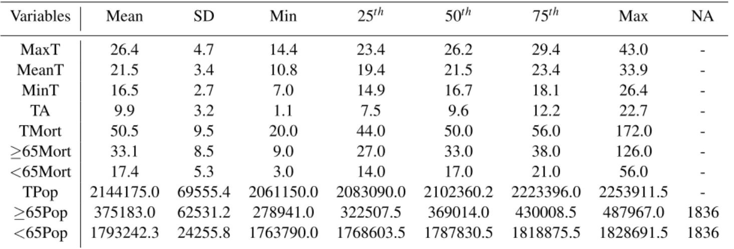
The descriptive statistics were obtained for all the variables described before, in section 2.1. Tables 3.1 and 3.2 present the mean; standard deviation (SD); minimum (Min); 25th, 50thand 75thpercentiles; maximum (Max) and number of missing values (NA) of the 10 previously described variables. All the values were rounded to one decimal place. Those statistics were obtained for the complete data set (all year) - Table 3.1 - and just for the summer period (May to September) - Table 3.2 -, both for the period between 1980 and 2017.
Table 3.1: Descriptive statistics of year-round data.
Variables Mean SD Min 25th 50th 75th Max NA
MaxT 21.3 6.1 6.5 16.2 20.5 25.7 43.0 12 MeanT 17.1 5.1 3.3 13.1 16.7 21.1 33.9 16 MinT 12.9 4.4 -1.0 9.7 13.0 16.4 26.4 11 TA 8.4 3.2 0.3 6.0 8.0 10.4 22.7 16 TMort 56.2 12.2 20.0 48.0 55.0 63.0 172.0 -≥65Mort 37.8 10.9 9.0 30.0 37.0 44.0 126.0 -<65Mort 18.4 5.6 3.0 14.0 18.0 22.0 56.0 -TPop 2144173.0 69552.8 2061150.0 2083090.0 2102360.2 2223396.0 2253911.5 -≥65Pop 375180.4 62529.5 278941.0 322507.5 365336.0 430008.5 487967.0 4383 <65Pop 1793241.9 24253.4 1763790.0 1768603.5 1784199.5 1818875.5 1828691.5 4383
The maximum temperature achieved in this period was 43oC which occurred on June 14 of 1981, the minimum temperature was -1oC on January 12 of 1985 and the thermal amplitude varied from 0.3
oC (7/12/1991) to 22.7oC (15/9/1992).
All mortality statistics are higher for the 65 years old or more population than the under 65 years old population; and the highest count of deaths, 172, occurred on June 15 of 1981, one day after the highest temperature registered.
The population statistics are very similar in both tables, because this data corresponds to annual average, so the values are the same for all days of each year.