A static approach to the Nelson-Siegel-Svensson model : an application for several negative yield cases

REM WORKING PAPER SERIES

A static approach to the Nelson-Siegel-Svensson model: an application

for several negative yield cases

Maria Teresa Medeiros Garcia and Vítor Hugo Ferreira Carvalho

REM Working Paper 035-2018

March 2018

REM – Research in Economics and Mathematics

Rua Miguel Lúpi 20, 1249-078 Lisboa,

Portugal

ISSN 2184-108X

Any opinions expressed are those of the authors and not those of REM. Short, up to two paragraphs can be cited provided that full credit is given to the authors.

1

A static approach to the Nelson-Siegel-Svensson model: an application for

several negative yield cases

Maria Teresa Medeiros Garcia a,b,* Vítor Hugo Ferreira Carvalho a

a _{ISEG – Lisbon School of Economics and Management, Universidade de Lisboa;} b_{REM – Research in Economics and Mathematics, UECE. UECE – Research Unit on}

Complexity and Economics is supported by Fundação para a Ciência e a Tecnologia.

* _{Correspondig author. Tel.: +351 213925993; fax: +351 - 213 971 196.}

E-mail addresses: mtgarcia@iseg.utl.pt (M. T. M. Garcia), vitorhugofc@aln.iseg.ulisboa.pt (V. Carvalho)

Abstract

The appearance of negative bond yields presents significant challenges for the fixed income markets, which mainly concern related forecasting models. The Nelson-Siegel-Svensson model (NSS) is one of the models that is most frequently used by central banks to estimate the term structure of interest rates.

The objective of this study is to evaluate the application of the NSS model to fit the yield curve of a set of 20 countries, the majority from the Eurozone, which registered negative sovereign bond yields. We conclude that the model adjusted well for all countries’ yield curves, although no changes or constraints were introduced. In addition, a comparison was carried out between market instantaneous interest rate and the interest rate for the very distant future, which the model can predict, with good results for the instantaneous interest rate. An evaluation of the possible behaviour of shared debt securities (i.e. Eurobonds) was also analysed.

In conclusion, the NSS model seems to remain a valuable, easy to use, and adaptable tool, to fit negative yield curves, for monetary policy institutions and market players alike.

2

JEL Classification: C02; C18; E43; E47; G12; G17

Key Words: yield curve; negative bond yields; Eurobonds; Nelson-Siegel-Svensson model

1 I

The existence of negative bond yields presents significant challenges for the fixed income markets. Some of these challenges are related to modelling and forecasting methods, and others are due to the actual size of assets with negative yields ($13,4 trillion, Financial Times, 2016). The final challenge is to detect the impact of negative bond yields on financial theory and the implications for bond holders and issuers.

As the Nelson and Siegel (NSS) model (1987) with the proposed extension of Svensson (1994) is adopted by central banks to estimate the term structure of interest rates (BIS, 2005), it is used in this study to evaluate how its adjustment behaviour fits the yield curves of a set of countries which registered negative sovereign bond yields which constitute an unusual situation.

Negative yields are a recent phenomona and to some degree can be an outcome of various important aspects. For example, the 2008 financial crisis led the Federal Reserve (Fed) to start quantitative easing programmes1 up until October 29th, 2014, which were later followed by the European Central Bank (ECB) (ECB, 2017a) in the aftermath of the 2010/2011 European government debt crisis and the significant reduction in the directorate interest rate of ECB. Japan led the fixed income markets to search for “safe

1 _{Available at:}

https://www.thebalance.com/what-is-quantitative-easing-definition-and-explanation-3305881 | https://www.ecb.europa.eu/explainers/show-me/html/app_infographic.en.html Accessed date: August 7th_{, 2017}

3

heavens”, as a result of its lost decades2 _{(Hayashi & Prescott, 2002) and low interest rates,}

compounded by reduction in GDP growth of China and world. These “safe heavens” issuers are those that have higher ratings and therefore they can provide a greater certainty that their debts wil be serviced entirely. In a certain way, the high debt levels of European Union countries, and the highest debts in the world, such as that of Japan (234% of GDP in 2015 - OECD, 2017), should demand greater yields for these issuers. However, ratings (that seem to be more favourable for developed countries (Cantor & Packer, 1996)) and the lack of the possibility for emerging countries to capture the fixed income markets with intensity, have led to the present situation, which is characterised by the issuers of higher debt in relatin to GDP, with, in some cases, the lowest yields, and, awkwardly, cases of negative yields, which are not so predictable and common.

Given that the market players (e.g. insurance companies, pension funds, and banks) need to estimate and model the term structure of interest rates with these recent negative bond yields, this study analyses the applicability of the use of the NSS model in this context, by means of friendly, widely-available, and simple tools. Accordingly, the objectives of this study are twofold. Firstly, to evaluate the adequacy of the NSS model through the fit of the yield curve, at a certain date, with at least one negative yield value and through the interest rates values that one can deduct from the model, compared with market data, with an easy-to-use approach. Secondly, to evaluate the results of the model with partial market bond yields data (short, intermediate and long-term).

The paper is comprised of the literature review, the methodology, the results and the conclusion sections. The literature review section presents and describes the NSS, its application and importance, and also the approaches carried out to fit negative yields

2 _{Hayashi and Prescott used the expression “Lost decade” to refer to the economic stagnation ofJapan in} the 1990s, due to low growth in productivity Although this term refers to the 1990s, the fall in real wages, low growth and persistant deflation, led to Japan implementing an economic stimulus, thus creating fiscal deficits and the highest level of debt in the world.

4

market data. In the methodology section, the NSS model and parameters are described in detail, as well as the calibration method, the analysis procedure, and the data and software definitions to accomplish data analysis. The results prepare the way for further research. Given that the majority of countries under study are European and in the Eurozone, a comparison is conducted between their yield curves and some effects of a possible future shared Eurozone debt security (i.e. Eurobonds). The conclusion section presents the main findings.

2 L

The term structure of interest rates, or yield curve, is a key variable of economics and finance (Büttler, 2007). The direct relation between term structure of interest rates and yield curve, should be clarified. Málek (2005), in Hladíková & Radová (2012), places the distinction to three equivalent descriptions of the term structure of interest rates:

 the discount function, which specifies zero-coupon bond prices as a function of maturity;

 the spot yield curve, which specifies zero-coupon bond yields (spot rates) as a function of maturity;

 the forward yield curve, which specifies zero-coupon bond forward yields (forward rates) as a function of maturity.

The discount function entails some undesirable conditions. Bond prices are insensitive to yields changes for shorter maturities. Sometimes, minimizing price errors, result in large yield errors for bonds for these shorter maturities (Svensson, 1994). Furthermore, monetary policy makers and economic discussions, generally focus on interest rates,

5

rather than prices (Geyer & Mader, 1999). For these reasons, the discount function cannot be a suitable description of the term structure of interest rates.

To the purpose of an entire evaluation of the yield curve (maturities can be as high as 30, 50, and even 100 years), the forward market products are not adequate, as they have a short time limit, and therefore the forward yield curve can only be a proper description of the yield curve for shorter maturities.

In the case of the spot yield curve, the market has no zero-coupon bonds for all maturities, and only a few sets of countries issue these instruments, so therefore coupon government bonds should be considered. The use of coupon bonds, with different coupon rates instead of zero-coupon bonds, have negligible impact, according to Kariya et al. (2013, in Inui, 2015). Svensson (1994) mentioned that obtaining implied forward interest rates from yield to maturity (YTM) on coupon bonds is more complicated than on zero coupon bonds. The YTM obtained from market data will give implied spot rates, instead of real spot rates, since one cannot compute the entire yield curve with all maturities (i.e. the spot yield curve) from zero-coupon bond yields, although Cox et al. (1985) stated that “the expectations hypothesis postulates that bonds are priced so that the implied forward rates are equal to the expected spot rates”. In synthesis, the term structure of interest rates, or the yield curve, is computed through the YTM of government coupon bonds, and through the YTM that will obtain the implied rates.

One of the objectives and usefulness of fit in the yield curve is to provide the monetary policy institutions with indicators of rates evolution and expectations (e.g. inflation). The need for monetary policy institutions to have these indicators increased when flexible exchange rates replaced fixed exchange rates (Svensson, 1994). Another significant purpose is related to fixed income market participants (e.g. hedging strategies, or assets allocation for pension funds).

6

There are several methods to fit the yield curve. Based on Sundaresan’s (2009) compilation, these include:

 the Vasicek (1977) model, which is a mean reversion process, which allows negative rates, but does not calibrate with market data;

 the Rendleman and Bartter (1980) model follows a simple multiplicative random walk. Rates are assumed to be lognormally distributed, which invalidates its use in the case of negative yields;

 the Cox, Ingersoll and Ross (CIR) model (Cox et al., 1985) is a mean reversion model, but it does not permit negative interest rates, neither does it calibrate with market data;

 the Ho and Lee (1986) model is calibrated to market yields and it assumes a normal distribution of interest rates, and interest rates can become negative;

 the Black, Derman and Toy (1990) (BDT) model can be calibrated through market equity options data, but it assumes that rates follow a lognormally distribution, which invalidates its use in the case of negative yields. It combines mean reversion and volatility;

 the Black and Karasinski (1991) model is calibrated to market yields and volatilities and separates mean reversion and volatility;

 the Nelson and Siegel (1987) and Svensson (1994) extension is an exponential function to approximate the unknown forward rate function;

 the Bootstrapping method generates a zero-coupon yield curve from existing market data such as bond prices, but lacks robustness (Martellini et al., 2003). It is beyond our purpose to evaluate all models in the context of negative yields. Therefore we decided to use the NSS model as the purpose of this study, in order to obtain a model that is calibrated with market data and also to evaluate the interest rates from the model

7

without evaluating volatilities for yields or bond prices, as is required in some other models. In fact, several curve fitting spline methods have been criticized for having undesirable economic properties and for being ‘black box’ models (Seber & Wild, 2003 in Annaert et al., 2010).

The NSS model is parsimonious and has been widely used in academia and in practice, however it is sensitive to the starting values of the parameters (𝛽_1,2,3,4and 𝛾1,2) (Annaert

et al., 2010).

The NSS model respects the restrictions imposed by the economic and financial theory (rates take real numbers and not complex ones, and are higher for longer terms, rather than for shorter ones) and considers any yield curve form which is empirically observed in the market (Diebold & Rudebusch, 2013, in Ibáñez, 2015). Furthermore, if the NSS behaves satisfactory in a negative yield market, then this would be of utmost importance for hedging strategies (mainly for market participants, to hedge against the flattening or steepening of the yield curve) and also for obtaining forecasts for interest rates levels (which is very useful for monetary policy makers). Accordingly, our purpose is to fit the yield curve and to obtain a static value of instantaneous interest rate (IIR) and the interest rate of a very distant future (IRVDF), and also to check if the values given by the model are in accordance with the market ones. Additionally, another objective is to use a friendly, widely-available tool for a not so in-depth user of maths tools or software.

3 M

The yield curve that can be estimated from bond yields of a certain economic region is of utmost importance for monetary and economic authorities to support decision processes

8

and to establish policies, as well as to market participants for their investments and actions (Martellini et al., 2003).

This study evaluates the NSS model, with a curve-fitting statistical model, under negative yields and all along the yield curve. This model provides values for instantaneous and distant future interest rates.

The approach adopted does not add more factors, parameters, or terms to the NSS model. It computes all yield curves for each of the selected countries and tries to obtain economic and financial data to evaluate the forecast adequacy of the model, even in cases of issuers with few negative yields. Therefore, an objective is not to consider the NSS model parameters time series, neither to forecast its values to obtain a yield curve evolution. A static fitting was adopted to check how the NSS model works with negative yields at some part of the yield curve.

The Nelson Siegel model and Svensson extension, Equation (1), is a parametric curve-fitting method procedure, which is statistical in its approach, and which generally does not have a sound economic foundation.

(1)

Svensson (1994) extension adds a new term, with a new decay parameter, Equation (2), to obtain a better fit.

(2)

As clearly described by Guedes (2008), the Nelson Siegel model parameters can have an economic interpretation. In this study, the interpretation of the parameters follows the Nelson Siegel model, namely:

𝜸(𝜽) = 𝜷𝟏+ 𝜷𝟐[ 𝟏 − 𝒆− 𝜽 𝝀𝟏 𝜽 𝝀𝟏 ] + 𝜷𝟑[ 𝟏 − 𝒆− 𝜽 𝝀𝟏 𝜽 𝝀𝟏 − 𝒆− 𝜽 𝝀_{𝟏] + 𝜷} 𝟒[ 𝟏 − 𝐞− 𝜽 𝝀𝟐 𝜽 𝝀_𝟐 − 𝒆− 𝜽 𝝀𝟐_] 𝜷𝟒[ 𝟏 − 𝐞− 𝜽 𝝀𝟐 𝜽 𝝀_𝟐 − 𝒆− 𝜽 𝝀𝟐_]

9

 () is the yield to maturity value (spot rate) at the time of data collection, with maturity ;

 β1 is the IRVDF;

 β1+β2 is the initial value of the curve and can be interpreted as the IIR;

 -β2 is the spread between the interest rates of long and short times (i.e. the average

slope of the curve);

 β1,2 and β3 determine how short and long interest rates interchange and are

responsible for the hump (inclination) that the yield curve shows.

 β4 is the extension of the model proposed by Svensson in 1994, which can be

interpreted as an independent decay parameter, which will introduce a new hump to fit the model better;

  is the maturity of the bond;

 1 and 2 are the parameters responsible for how inclination and curvature behave,

which does not have an economic interpretation, although determine the interchange between short and long interest rates.

Until negative bond yields appear in some markets, the NSS model did not present much difficulty in its application and is thus widely used.

Guedes (2008) stated that 𝛽₁+ 𝛽₂ > 0, which for the paradigm of that time and up until then appeared to be a very reasonable economic and financial condition. The general perception that rates, or at least nominal rates (real rates, which consider other effects, such as inflation, can be lower than zero) would always be positive, leading to the definition of limits under which the model should work. However, time and markets have shown that 𝛽₁+ 𝛽₂ (interpreted as the IIR) can be lower than zero. This study tries to show that there is an economical and real-world interpretation for 𝛽₁+ 𝛽₂ < 0.

10

For a first approach, it is expected that the yield curve fitting with some negative bond yields would be more difficult, due to the calibration process, which usually calculates the minimum value of the sum of squared residuals (SSR). As stated by Svensson (1994), the parameters are obtained by minimizing the sum of squared yield errors between estimated and observed yields. Our analysis follows the NSS model and the SSR. Gilli et al. (2010) stated that one possibility for the calibration is to use Equation (3) to calculate the SSR, where y is estimated yield using the NSS model, and yM is the market yield value:

(3) 𝑚𝑖𝑛

𝛽,𝜆 ∑(𝑦 − 𝑦 𝑀₎2

In this study, the market values are the bond yields for each maturity, for each country. Using the Microsoft Excel Solver (Frontline System, 2017a) function, we obtain the residuals’ minimum value, which allows one to obtain the values of the parameters 𝛽_1,2,3,4and 𝛾1,2. The parametrization of Solver for the data used in this paper is presented

in detail in Section 3.2.

For forecasting purposes, only a few market bond yields maturities where tested, and the NSS model was used to adjust the curve for the missing maturities. Partial market data was considered following the classification of the beginning of the 1990s, that bond markets used for bond maturities, namely: short, intermediate, and long term (Martellini et al, 2003). The most usual time frame for each division are as follow: bonds with maturities until 5 years are called short-term bonds; from 5 to 10/12 years they are called intermediate bonds, and; higher than 10/12 years are called long bonds.

When the NSS model was used for forecasting short-term maturity bonds, the 5 years’ time frame wasnot considered as a fixed period, because the model does not produce good-fitting data. The NSS model seems to need at least one negative yield market data

11

to proceed with proper calibration. Taking this into consideration, the short-term time frame was different for every country, ranging from 2 to 5 years.

The inferior limit of the intermediate period is defined by the higher value found from the short-term forecast (STF). The upper limit was defined by the best-observed fitting, but whenever possible, this was no more than 10 years (Lithuania is a special case, as it has no bonds with maturities higher than 7 years), and the wider period that was considered with no market data to calibrate the model (Switzerland is a special case, where the limit is 25 years).

The adequacy of the NSS model to obtain accurate enough parameter values with partial market data was evaluated for 3 sectors of the yield curve: short, intermediate, and long term.

For STF, the model was calibrated only with market yields for intermediate and long-term maturities, and thus obtained different values for the parameters to the ones obtained when all the market data was used to calibrate the model. The parameters values and the countries’ yields curves with lower forecasts can be assessed in Appendix II. Similarly, the same action was carried out when calculating the intermediate and long-term maturities forecasts. For each of the forecast maturities, the model only had access to the other maturities, for which the values of the factors that best fitted the curve were computed. The Solver function was run as many times as possible, in order to get the best forecast fit values.

3.1 D

The study considers a set of 304 different government bonds, from a group of 20 countries (Austria, Belgium, Bulgaria, the Czech Republic, Denmark, Finland, France, Germany, Ireland, Italy, Japan, Lithuania, Luxembourg, the Netherlands, Portugal, Slovakia,

12

Slovenia, Spain, Sweden, and Switzerland) with at least one negative yield to maturity government bond at the date of data collection. These dates were: March 15th, 2017, for Austria, Denmark, Finland, France, the Netherlands, Sweden and Switzerland; March 16th_{, 2017, for Germany and Japan, and; May 5}th_{, 2017, for Belgium, Bulgaria, the Czech}

Republic, Ireland, Italy, Lithuania, Luxembourg, Portugal, Slovakia, Slovenia and Spain. The data source used to obtain bonds information used in the study was Bloomberg, through a Bloomberg Terminal. Inflation indexed bonds were not considered.

After evaluating the NSS model for the entire yield curve of those countries whose data was gathered on March 15th _{and 16}th_{, 2017, the set of issuers was extended to incorporate}

the other 11 countries that presented negative yield to maturity on May 5th, 2017. The number of study countries was chosen taking into consideration two main purposes: first, to try to get more issuers to evaluate model adequacy for a wider set of data, and; second, because in the second set of countries, most are from Europe and are subject to the ECB monetary policy, in order to try and obtain a wider, detailed sample, and if possible, to obtain a conclusion that could apply to Europe and/or the Eurozone.

From the 19 countries that currently comprise the Eurozone (European Union, 2017 – which use the Euro as their official currency and are subject to ther ECB monetary policy), 14 are included in this study. The other 5 Eurozone countries (Cyprus, Estonia, Greece, Latvia, and Malta) were not included in the study, as they did not manifest any fixed income security with a negative yield, during the study periods of March 15th and 16th_{, 2017 and May 5}th_{, 2017.}

At present, the European Union has 28 members (European Union, 2017), and therefore half of the members had negative bond yields at the time of the study dates. Croatia had negative yields for the period of the end of 2016 to the beginning of 2017, although by the time of data collection (May 5th, 2017), yields for all maturities were positive.

13

Table I and Figure 1 show how many different securities were used for each country, as well as the denomination of their currencies.

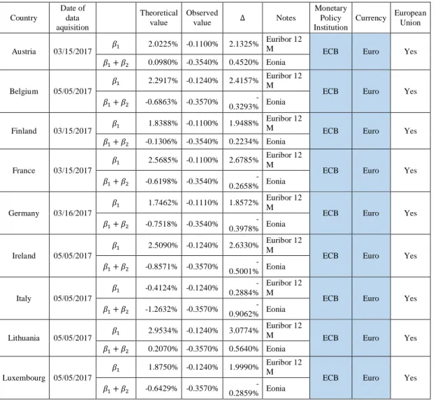
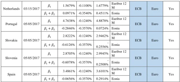
Tables II and III show the countries included in the study, their date of data collection, the corresponding monetary policy institution, the currency, whether the country belongs to the European Union, the β1 and β1+β2 theoretical values (obtained from the fitting

process), the observed values, and explanatory notes.

Table I. Number of bonds per country

Countries Number of bonds Situation Currency

Austria 16 Included EUR

Belgium 14 Included EUR

Bulgaria 9 Included BGN

Croatia 9 Excluded HRK

Czech Republic 12 Included CZK

Denmark 6 Included DKK

Finland 12 Included EUR

France 26 Included EUR

Germany 38 Included EUR

Ireland 12 Included EUR

Italy 15 Included EUR

Japan 18 Included JPY

Lithuania 11 Included EUR

Luxembourg 6 Included EUR

Netherlands 14 Included EUR

Portugal 13 Included EUR

Slovakia 12 Included EUR

Slovenia 13 Included EUR

Spain 15 Included EUR

Sweden 16 Included SEK

Switzerland 17 Included CHF

Total 304

Figure 1. Number of bonds per currency

Table II presents all countries subject to the ECB monetary policy, which use the Euro as their currency. These countries share the same currency risk and the same rates’

14

referential. Table III displays all the other cases, including Bulgaria, the Czech Republic, Denmark and Sweden, as these countries determine their interest rates independently from the ECB, and are able to control their currency exchange rate (Bulgaria has a fixed exchange rate pegged to the Euro).

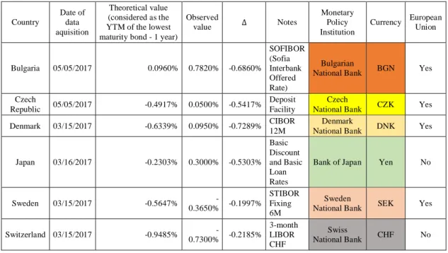
Tables IV and V show, for the two sets of countries, the data if the theoretical value for the IRVDF considered is the yield to maturity of the lowest maturity bond (1 year). Tables VI and VII show the data if the observed value for the IRVDF considered is the yield to maturity of the highest maturity bond.

3.2 A

The application of the Solver function to all bonds of the countries took into consideration the following conditions: a GRG nonlinear algorithm for the resolution method3; a restriction precision value of 10-8 _{(the standard value used by Solver is 10}-6_{, whereby a}

lower value provides a more precise value, although this increases the time Solver spends to arrive at a solution); the default selection for Solver to use automatic rounding was used; the value chosen for the Convergence (value between 0 and 1) was 10-8_{, which}

defines the upper limit for the relative change in the destiny cell, for the last 5 iterations; a criteria for Solver to stop (i.e., if during the last 5 iterations the relative change in the value of the destination cell is less than 10-6%, then Solver stops trying to converge even more) (Microsoft, 2017a).

The results obtained with direct differentiation (default on Solver) for all yield curves fitting computation were very good.

15

Solver uses a Generalised Reduced Gradient algorithm for optimising non-linear problems (Microsoft, 2017b), which provides a locally-optimal solution for a reasonably well-scaled, non-convex model (Frontline System, 2017b). Function f is convex, if the function f is below any line segment between two points on f. Figure 2 is an adaptation from Tomioka (2012), which provides an example of the convex and non-convex function.

Figure 2. Convex and non-convex function

The starting values for 𝛽_1,2,3,4and 𝛾1,2 should be in, or as near as possible, the order of

magnitude of the expected values. Values near, or below 0.01 for 𝛽_𝑖 and 1 to 𝛾𝑗were used.

After the first solution provided by Solver, the parameters values were submitted to small changes and the Solver function was ran again, to obtain a SSR as low as possible. Only when Solver provided the message that after 5 iterations the fitting curve had not changed, was that solution considered as the final one. No restrictions were applied to any of the values that 𝛽_1,2,3,4and 𝛾1,2. assumed.

When modelling the entire yield curve, using the NSS model to access all the market yields to obtain SSR, or when modelling the entire yield curve, with part of the market data available (i.e. the cases of short-term, intermediate and long-term, bonds maturities), the parameters 𝛽_1,2,3,4and 𝛾1,2. could take any value, and no restriction was applied to

them. The parameters values obtained for each country are shown in Table VIII (NSS model used all market yields available), Table IX (short-term maturities forecast, or simply STF), Table X (intermediate term maturities forecast or simply, intermediate-term

16

forecast (ITF)), and Table XI (long-term maturities forecast, or simply, long-term forecast (LTF)).

It has been referred to above that β1 can be interpreted as the IRVDF, and β1+β2 as the

IIR. In this study, the IIR considered is the overnight rate (in practice, the instantaneous rate can be identified with an overnight forward rate (Svensson, 1994)) supervised by the countries’ monetary policy institution. For countries subject to ECB rules, the rate considered is the unsecured overnight lending rate, Eonia®4 (Euro OverNight Index Average). Eonia® is the observed value that compares the theoretical obtained from the NSS model.

The definition of a very distant future and its correspondent interest rate for that time horizon is, in a certain way, not concrete date. Due to the present market situation of the ECB monetary-easing policy that is intended to run until the end of December 2017, or beyond, if necessary (ECB, 2017b), and considering the most time-distant rate at which Euro interbank term deposits are offered Euribor®5 _{12 months, this was the rate chosen}

as the observed value to compare with β1.

In Table III, due to the uniqueness of each country’s monetary policy institution, the rates considered to be the benchmark for β1 (IRVDF) and β1+β2 (IIR) are diversified. For β1+β2

the corresponding overnight rate was chosen, or the repo rate, with the shorter time horizon (a repo rate is the rate at which banks can borrow from their Central bank). Hladíková & Radová (2012) also used the repo rate to compare with the starting value of the estimated forward rate. These two rates are very close to each other (Martellini et al., 2003). Similarly, for β1 (IRVDF), the corresponding rate equivalent to the country´s

Euribor was chosen.

4 _{Available at: https://www.emmi-benchmarks.eu/euribor-eonia-org/eonia-rates.html Accessed date:} August 6th_{, 2017}

5 _{Available at: https://www.emmi-benchmarks.eu/euribor-org/about-euribor.html Accessed date:} August 6th_{, 2017}

17

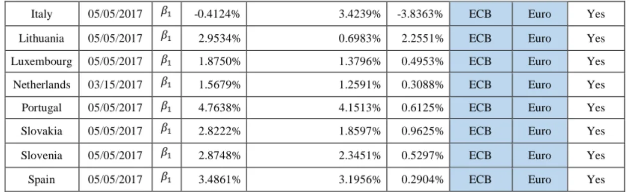
Theoretical and observed IRVDF and IIR can be compared in Figures 3 and 4, and also Tables II and III. As mentioned above, the definition of very distant future is not concrete, and thus the following two changes were considered when evaluating the data and for the analysis;

 theoretical value, considered as being the YTM of the lowest maturity bond (1 year). Data can be assessed in Tables IV and V, and Figure 5.

 observed value, considered as being the YTM of the highest maturity bond. Data can be assessed in Tables VI and VII, and Figure 6.

A descriptive statistical analysis (with the calculation of: mean, median, standard deviation, kurtosis, asymmetry, minimum and maximum) was carried out for the differences of the theoretical and observed values. This exercise, together with a comparison between theoretical and observed values, can help obtain more substantiated conclusions. This analysis was applied to the two sets of countries’ data (all the study countries, and then the subset of countries supervised by the ECB), for both the IIR and the IRVDF.

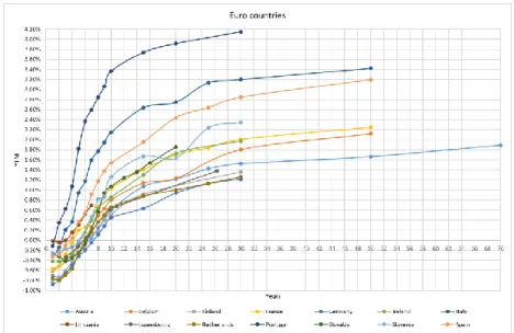
As the majority of countries in the study are from Europe, we compared all yield curves (Figure 7) for these issuers. The spectrum of maturities that each country chooses, or can have access to, in the market, is very different, as are the yields that each can have, and it is very wide. The differences for the yield curves are related to the premiums required by the market and they are dependent on ratings, political risk, GDP growth, debt levels, and economic development, among other variables.

10-year maturity bonds yield is one of the most used and widely-compared one in financial markets. For the set of European countries, only Lithuania did not have maturities higher than 7 years, and thus it cannot be compared with its fellow European countries.

18

Figure 3. Theoretical and observed IIR Figure 4. IRVDF (with observed value considered as Euribor 12 M)

Figure 5. IRVDF (with theoretical value considered as the YTM of the lowest maturity bond (1 year))

Figure 6. IRVDF (with observed value considered as the YTM of the highest maturity bond)

As a theoretical exercise, if the Eurozone countries eventually agreed on a shared debt security (i.e. Eurobonds), bonds with 10 year maturities could be issued at an initial phase, with higher maturities (>10 years) being just the choice of each country. Figure 8 shows this set of countries (without Lithuania) and their yield curves.

20

Figure 7. European countries yield curves

Figure 8. European countries yield curves (maturities until 10 years)

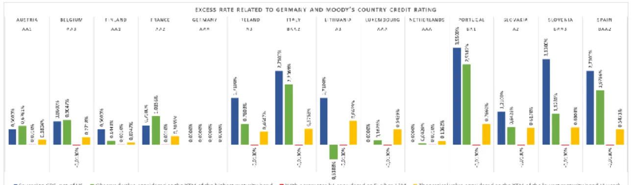
For the Eurozone countries, it was analysed whether the differences between the theoretical and observed rates values, for β1 (IRVDF), could be explained by the excess

rate that each country has in relation to Germany (as Germany has the highest credit rating and its Sovereign CDS, net of US, is 0.00%)6_{, using the Moody´s credit ratings, for each}

country.

Figure 9 shows the differences between the theoretical and observed rates values, for β1

(IRVDF), for two interpretations of the very distant future. The first difference is the

6 _{Available at: http://pages.stern.nyu.edu/~adamodar/New_Home_Page/datafile/ctryprem.html} Accessed date: June 10th_{, 2017}

21

comparison between Sovereign CDS, net of US (or net of Germany, as both have the same value) (blue bar), and the observed value for β1, considered as the YTM of the

highest maturity bond (green bar). For example, the excess rate for Portugal in relation to Germany is 2.9342%, which means that the YTM of its highest maturity bond is 2.9342% higher than the YTM of the highest maturity bond of Germany, with the relation with the Sovereign CDS, net of US, being of the same sign and similar value.

The second difference is between the observed value for the β1 parameter (considered as

Euribor at 12 Months) and its difference in relation to Germany’s observed value (also, Euribor at 12 Months) (red bar); and the difference between the theoretical value for β1

(considered as YTM of the lowest maturity bonds, 1 year) for each country and Germany (yellow bar).

Figure 9. Excess rate related to Germany

4 R

The NSS model fitting process, applying no restrictions on the parameters values, adjusts the yield curve well for the wide variety of countries and range of maturities (Appendix II).

It was pointed out that the application of the Nelson-Siegel model was not appropriate for the Japanese Government Bonds market, because it might show a negative interest rate

22

and an abnormal shape in the short- term region (Kikuchi & Shintani, 2012, in Inui, 2015). In this study, using the NSS model, the curve shows a good fitting (Figure 20), and the difference between the short interest rate, chosen as the observed value, and the theoretical interest rate is 0.044%, which is a low value (Table III).

The values obtained for β1 and β1+β2, interpreted as IRVDF (Figure 4, and Tables II and

III) and IIR respectively (Figure 3, and Tables II and III), show that theoretical and observed values are closer to each other for the IIR, than for the IRVDF, which presents a wider difference.

If the observed value for the IRVDF is considered as the highest maturity of the YTM, then the values are very close to the theoretical ones. Specifically, the excess rate related to Germany can be almost fully explained.

The difference between theoretical and observed IIR, for the all sets of countries, has an almost normal distribution (kurtosis=3.14) with: a mean of -0.055%, a median of 0.019%, a standard deviation of 0.644%, a minimum of -1.926%, and a maximum of 1.233%. These results show a very wide range, which is probably influenced by different monetary policies. The same values, for the countries subject to the ECB monetary policy, show a platykurtic distribution (kurtosis=-067) with: a mean of -0.081%, a median of -0.251%, a standard deviation of 0.429%, a minimum of -0.906%, and a maximum of 0.564%, which represents a shorter range, suggesting the same monetary policy.

The difference between theoretical and observed IRVDF, for all the sets of countries, has a leptokurtic distribution (kurtosis=5.92), with: a mean of 2.058%, a median of 2.274%, a standard deviation of 1.688%, a minimum of -3.501%, and a maximum of 4.888%, showing significant dispersion. The same values for the countries subject to the ECB monetary policy show a platykurtic distribution (kurtosis=2.69), with: a mean of 2.470%,

23

a median of 2.524%, a standard deviation of 1.154%, a minimum of -0.288%, and a maximum of 4.888%, which also shows a wide range.

The NSS model theoretical values for β1 (IRVDF) are generally the value of the yield of

the longest maturity in the yield curve (except for the extreme cases of Bulgaria, Italy, Lithuania and Sweden). To a certain degree, this is the most very distant future that is available for each country, and therefore, if the highest maturity for each country is the market interpretation of very distant future, then the model provides good values. Otherwise, if for very distant future one considers the one-year time frame, then the model is not an appropriate one.

The results for short, intermediate, and long-term forecasts, can be assessed, respectively in Appendices II, III and IV. The short-term forecast shows that the model has difficulty in fitting the yield curve, given that the beginning of the yield curves is less smooth than the intermediate and long terms. Furthemore, negative yields appear in the shorter term. The intermediate and long-term forecasts show very acceptable fittings, in some cases with very few maturities that the NSS model can adjust for the entire curve.

Considering the subset of countries and yield curves that can be observed in Figure 8, and if a shared debt security (i.e. Eurobonds) issue was eventually to be carried out, then the market would, theoretically, lower the risk premium and the yields for the most stressed countries (those that show higher yields). For the lower risk premium issuers, this will increase yields. Since all countries share the risk, these risk premiums are thus reflected in yields, which could be a price to pay to obtain a more equal and less stressful financial system in the Eurozone.

Figure 9 shows the evaluation of rate differences related to the excess rate of Germany, whereby there is a clear relationship between excess rate observed and Sovereign CDS, net of US, at least for the majority of countries considered. Only in the case of Ireland,

24

Lithuania and Slovenia, are the differences higher than 1%. The excess rate related to Germany is well explained.

5 C

The application of the NSS model to 20 countries with negative yields gives good estimates of the entire yield curves, fitting the data well. The methodology used is friendly and can be used as a simple and widely-available tool.

The forecast of the IIR seems to be good, as the differences between theoretical and observed values appear to be small. If the IRVDF is considered to be the rate at the highest bond maturity, then the model presents good values.

The interpretation of the parameters of the NSS model seems to be adequate.

In the case of countries subject to the ECB monetary policy, the interest rate is defined by the ECB, however, in practice, European countries in the Eurozone are very different in essence (e.g., economic models, debt levels, financial history, weight, and importance on financial markets). Accordingly, all are expected to have the same rates from the model, which seems not be a realistic hypothesis. It can be concluded that rates should not all be the same, as the market requests a country risk premium (CRP) for each rate, which is related to their ratings, debt level, GDP, national budgets and deficits, and political risk, among other factors. If the Eurozone countries had the same debt securities, such as Eurobonds, then rates would be the same, and the yield curve would be only one, and therefore the expected rate values obtained using the NSS model would be more precise and a good proxy for the market participants.

The excess rate in relation to Germany, calculated from Moody´s ratings and the corresponding Sovereign CDS, net of US (or Germany, as both countries share the same

25

value), for countries subject to the ECB monetary policy, can be explained from the model parameters, when considering the IRVDF to be the yield to maturity of the highest maturity for that country. Those countries that presented a difference higher than 1%, are Ireland, Lithuania and Slovenia.

The forecast outputs show good fitting data for real values for both intermediate-term and long-term maturities. On the other hand, short-term forecasted values are not as accurate as expected, which leads to the conclusion that, in this case, it is not a good model. The reasons for this can be the instability of monetary policy and the volatility of short-term interest rates.

In conclusion, the NSS model seems to be a valuable, easy-to-use, and adaptable tool, to fit the yield curve with negative yields, which is available for monetary policy institutions and market players alike.

6 R

Annaert, J., Claes, A., Ceuster, M., Zhang, H. (2010). Estimating the Yield Curve Using

the Nelson-Siegel Model – A Ridge Regression Approach, Universiteit Antwerpen.

BIS (2005). Zero-coupon yield curves: technical documentation, BIS Papers, 25, Bank for International Settlements.

Büttler, H. (2007). An Orthogonal Polynomial Approach to Estimate the Term Structure

of Interest Rates, Swiss National Bank Working Papers, 8.

Cantor, R. & Packer, F. (1996). Determinants and Impact of Sovereign Credit Ratings, Federal Reserve Bank of New York, 37-53.

26

Cox, J. C., Ingersoll, J. E., Ross, S. A. (1985). A Theory of the Term Structure of Interest

Rates, Econometrica, 53 (2), 385-407.

ECB (2017a). Asset purchase programmes. Available at:

https://www.ecb.europa.eu/mopo/implement/omt/html/index.en.html [Accessed date: August 7th, 2017].

ECB (2017b). Monetary policy decisions. Press Release, 20 July 2017. Available at: https://www.ecb.europa.eu/press/pr/date/2017/html/ecb.mp170720.en.html

[Accessed date: August 6th, 2017].

European Union (2017). EU monetary cooperation. Available at:

https://europa.eu/european-union/about-eu/money/euro_en [Accessed date: March 15th_{, 2017].}

Financial Times (2016). Value of negative-yielding bonds hits $13.4tn. Available at: https://www.ft.com/content/973b6060-60ce-11e6-ae3f-77baadeb1c93?mhq5j=e3 [Accessed date: July 2nd_{, 2017].}

Frontline Systems (2017a). Excel Solver Online Help. Available at: https://www.solver.com/excel-solver-online-help [Accessed date: August 8th_,

2017].

Frontline Systems (2017b). Excel Solver – GRG Nonlinear Solving Method Stopping

Conditions. Available at: https://www.solver.com/excel-solver-grg-nonlinear-solving-method-stopping-conditions [Accessed date: June 15th, 2017].

Geyer, A. & Mader, R. (1999). Estimation of the Term Structure of Interest Rates – A

Parametric Approach, Oesterreichische Nationalbank Working Paper 37.

Gilli, M., Große, S. and Schumann, E. (2010). Calibrating the Nelson-Siegel-Svensson

27

Guedes, J. (2008). Modelos Dinâmicos da Estrutura de Prazo das Taxas de Juro, IGCP Instituto de Gestão da Tesouraria e do Crédito Público, I. P..

Hayashi, F. & Prescott, E. C. (2002). The 1990s in Japan: A Lost Decade, Review of Economic Dynamics, 5 (1), 206-235.

Hladíková, H. & Radová, J. (2012). Term Structure Modelling by Using Nelson-Siegel

Model, European Financial and Accounting Journal, 7 (2), 36-55.

Ibáñez, F. (2015). Calibrating the Dynamic Nelson-Siegel Model: A Practitioner

Approach, Central Bank of Chile.

Inui, K. (2015). Improving Nelson-Siegel term structure model under zero / super-low

interest rate policy, Meiji University.

Martellini, L., Priaulet, P. and Priaulet, S. (2003). Fixed-Income Securities Valuation,

Risk Management and Portfolio Strategies, Wiley.

Microsoft (2017a). Função SolverOptions. Available at: https://msdn.microsoft.com/pt-br/library/office/ff195446.aspx [Accessed date: June 15th_{, 2017].}

Microsoft (2017b). Solver Uses Generalized Reduced Gradient Algorithm. Available at: https://support.microsoft.com/en-us/help/82890/solver-uses-generalized-reduced-gradient-algorithm [Accessed date: July 2nd, 2017].

Nelson, C. & Siegel, A. (1987). Parsimonious Modelling of Yield Curve, Journal of

Business, 60, 473-489.

OECD (2017). General government debt (indicator). doi: 10.1787/a0528cc2-en; Available at: https://data.oecd.org/gga/general-government-debt.htm [Accessed date: June 17th, 2017].

Sundaresan, S. (2009). Fixed Income Markets and Their Derivatives, Academic Press, Third Edition.

28

Svensson, L. E. (1994). Estimating and Interpreting Forward Interest Rates: Sweden 1992-1994, Centre for Economic Policy Research Discussion Paper 1051.

Tomioka, R. (2012). Convex Optimization: Old Tricks for New Problems, The University of Tokyo, DTU PhD Summer Course.

A

A

I.

Table II. Data subject to the ECB monetary policy

Country Date of data aquisition Theoretical value Observed value ∆ Notes Monetary Policy Institution Currency European Union Austria 03/15/2017 𝛽1 2.0225% -0.1100% 2.1325% Euribor 12

M _{ECB Euro Yes}

𝛽1+ 𝛽2 0.0980% -0.3540% 0.4520% Eonia

Belgium 05/05/2017

𝛽1 2.2917% -0.1240% 2.4157% Euribor 12 _M

ECB Euro Yes 𝛽1+ 𝛽2 -0.6863% -0.3570% _0.3293% - Eonia

Finland 03/15/2017 𝛽1 1.8388% -0.1100% 1.9488%

Euribor 12

M _{ECB Euro Yes}

𝛽1+ 𝛽2 -0.1306% -0.3540% 0.2234% Eonia

France 03/15/2017

𝛽1 2.5685% -0.1100% 2.6785% Euribor 12 _M

ECB Euro Yes 𝛽1+ 𝛽2 -0.6198% -0.3540%

-0.2658% Eonia Germany 03/16/2017

𝛽1 1.7462% -0.1110% 1.8572% Euribor 12 _M

ECB Euro Yes 𝛽1+ 𝛽2 -0.7518% -0.3540% _0.3978% - Eonia

Ireland 05/05/2017

𝛽1 2.5090% -0.1240% 2.6330%

Euribor 12 M

ECB Euro Yes 𝛽1+ 𝛽2 -0.8571% -0.3570% _0.5001% - Eonia Italy 05/05/2017 𝛽1 -0.4124% -0.1240% -0.2884% Euribor 12 M

ECB Euro Yes 𝛽1+ 𝛽2 -1.2632% -0.3570% _0.9062% - Eonia

Lithuania 05/05/2017 𝛽1 2.9534% -0.1240% 3.0774%

Euribor 12

M _{ECB Euro Yes}

𝛽1+ 𝛽2 0.2070% -0.3570% 0.5640% Eonia

Luxembourg 05/05/2017

𝛽1 1.8750% -0.1240% 1.9990% Euribor 12 _M

ECB Euro Yes 𝛽1+ 𝛽2 -0.6429% -0.3570%

-0.2859% Eonia

29

Netherlands 03/15/2017 𝛽1 1.5679% -0.1100% 1.6779%

Euribor 12

M _{ECB Euro Yes}

𝛽1+ 𝛽2 0.0971% -0.3540% 0.4511% Eonia

Portugal 05/05/2017 𝛽1

4.7638% -0.1240% 4.8878% Euribor 12

M _{ECB Euro Yes}

𝛽1+ 𝛽2 -0.2846% -0.3570% 0.0724% Eonia

Slovakia 05/05/2017

𝛽1 2.8222% -0.1240% 2.9462%

Euribor 12 M

ECB Euro Yes 𝛽1+ 𝛽2 -0.6126% -0.3570% _0.2556% - Eonia

Slovenia 05/05/2017

𝛽1 2.8705% -0.1240% 2.9945%

Euribor 12 M

ECB Euro Yes 𝛽1+ 𝛽2 -0.6078% -0.3570% _0.2508% - Eonia

Spain 05/05/2017 𝛽1 3.4861% -0.1240% 3.6101%

Euribor 12

M _{ECB Euro Yes}

𝛽1+ 𝛽2 -0.0656% -0.3570% 0.2914% Eonia

Table III. Data not subject to the ECB monetary policy

Country Date of data aquisition Theoretical value Observed value ∆ Notes Monetary Policy Institution Currency European Union Bulgaria 05/05/2017 𝛽1 -2.7195% 0.782% _3.5015% -SOFIBOR (Sofia Interbank

Offered Rate) Bulgarian National Bank BGN Yes 𝛽1+ 𝛽2 0.8329% _0.4000% - 1.2329% LEONIA (LEv OverNight Index Average) Reference Rate Czech Republic 05/05/2017

𝛽1 2.8872% 0.0500% 2.8372% Deposit Facility Czech

National Bank CZK Yes 𝛽1+ 𝛽2 -1.8763% 0.0500% _1.9263% - 2W repo rate Denmark 03/15/2017 𝛽1 1.7728% 0.0950% 1.6778% CIBOR 12M Denmark National Bank DNK Yes 𝛽1+ 𝛽2 -0.1107% _0.4857% - 0.3750% Tomorrow/next _{(T/N) Rate} Japan 03/16/2017 𝛽1 1.3822% 0.3000% 1.0822% Basic Discount Rates and Basic Loan Rates Bank of Japan Yen No 𝛽1+ 𝛽2 0.0010% _0.0430% - 0.0440% Average value of Uncollateralized Overnight Call Rate for Mar. 16 Sweden 03/15/2017

𝛽1 2.8118% _0.3650% - 3.1768% STIBOR Fixing _6M Sweden

National Bank SEK Yes 𝛽1+ 𝛽2 -0.1883% _0.5000% - 0.3117% Repo rate Switzerland 03/15/2017 𝛽1 0.5743% _0.7300% - 1.3043% 3-month LIBOR _CHF Swiss National Bank CHF No 𝛽1+ 𝛽2 -0.7354% -0.7300% -0.0054% SARON (formerly repo overnight index (SNB))

Table IV. Data subject to the ECB monetary policy (theoretical value considered as the YTM of the lowest maturity bond - 1 year) – IRVDF

Country Date of data aquisition Theoretical value (considered as the YTM of the lowest maturity bond - 1 year)

Observed value ∆ Notes Monetary Policy Institution Currency European Union Austria 03/15/2017 -0.7037% -0.1100% -0.5937% Euribor _12M ECB Euro Yes Belgium 05/05/2017 -0.6123% -0.1240% -0.4883% Euribor

30

Finland 03/15/2017 -0.8094% -0.1100% -0.6994% Euribor

12M ECB Euro Yes France 03/15/2017 -0.5786% -0.1100% -0.4686% Euribor _12M ECB Euro Yes Germany 03/16/2017 -0.8841% -0.1110% -0.7731% Euribor

12M ECB Euro Yes Ireland 05/05/2017 -0.4194% -0.1240% -0.2954% Euribor

12M ECB Euro Yes Italy 05/05/2017 -0.3088% -0.1240% -0.1848% Euribor

12M ECB Euro Yes Lithuania 05/05/2017 -0.0152% -0.1240% 0.1088% Euribor

12M ECB Euro Yes Luxembourg 05/05/2017 -0.3402% -0.1240% -0.2162% Euribor _12M ECB Euro Yes

Netherlands 03/15/2017 -0.7479% -0.1100% -0.6379% Euribor

12M ECB Euro Yes Portugal 05/05/2017 -0.1181% -0.1240% 0.0059% Euribor

12M ECB Euro Yes Slovakia 05/05/2017 -0.2671% -0.1240% -0.1431% Euribor

12M ECB Euro Yes Slovenia 05/05/2017 -0.2533% -0.1240% -0.1293% Euribor

12M ECB Euro Yes Spain 05/05/2017 -0.3368% -0.1240% -0.2128% Euribor _12M ECB Euro Yes Table V. Data not subject to the ECB monetary policy (theoretical value considered as the YTM of the lowest

maturity bond - 1 year) – IRVDF

Country Date of data aquisition Theoretical value (considered as the YTM of the lowest maturity bond - 1 year)

Observed value ∆ Notes Monetary Policy Institution Currency European Union Bulgaria 05/05/2017 0.0960% 0.7820% -0.6860% SOFIBOR (Sofia Interbank Offered Rate) Bulgarian

National Bank BGN Yes Czech

Republic 05/05/2017 -0.4917% 0.0500% -0.5417% Deposit Facility

Czech

National Bank CZK Yes Denmark 03/15/2017 -0.6339% 0.0950% -0.7289% CIBOR _{12M National Bank} Denmark DNK Yes

Japan 03/16/2017 -0.2303% 0.3000% -0.5303% Basic Discount and Basic Loan Rates

Bank of Japan Yen No

Sweden 03/15/2017 -0.5647% -0.3650% -0.1997% STIBOR Fixing 6M Sweden

National Bank SEK Yes Switzerland 03/15/2017 -0.9485% -0.7300% -0.2185% 3-month LIBOR CHF Swiss National Bank CHF No Table VI. Data subject to the ECB monetary policy (observed value considered as the YTM of the highest maturity

bond - 1 year) – IRVDF

Country Date of data aquisition

Theoretical value

Observed value (considered as the YTM of the highest maturity bond)

∆ Monetary Policy Institution Currency European Union Austria 03/15/2017 𝛽1 2.0225% 1.8931% 0.1294% ECB Euro Yes Belgium 05/05/2017 𝛽1 2.2917% 2.1217% 0.1700% ECB Euro Yes Finland 03/15/2017 𝛽1 1.8388% 1.3619% 0.4769% ECB Euro Yes France 03/15/2017 𝛽1 2.5685% 2.2526% 0.3158% ECB Euro Yes Germany 03/16/2017 𝛽1 1.7462% 1.2170% 0.5291% ECB Euro Yes Ireland 05/05/2017 𝛽1 _{2.5090% 1.9774% 0.5317% ECB Euro Yes}

31

Italy 05/05/2017 𝛽1 _{-0.4124% 3.4239% -3.8363% ECB Euro Yes}

Lithuania 05/05/2017 𝛽1 2.9534% 0.6983% 2.2551% ECB Euro Yes Luxembourg 05/05/2017 𝛽1 1.8750% 1.3796% 0.4953% ECB Euro Yes Netherlands 03/15/2017 𝛽1 _{1.5679% 1.2591% 0.3088% ECB Euro Yes}

Portugal 05/05/2017 𝛽1 4.7638% 4.1513% 0.6125% ECB Euro Yes Slovakia 05/05/2017 𝛽1 2.8222% 1.8597% 0.9625% ECB Euro Yes Slovenia 05/05/2017 𝛽1 _{2.8748% 2.3451% 0.5297% ECB Euro Yes}

Spain 05/05/2017 𝛽1 3.4861% 3.1956% 0.2904% ECB Euro Yes Table VII. Data not subject to the ECB monetary policy (observed value considered as the YTM of the highest

maturity bond - 1 year) – IRVDF

Country Date of data _aquisition Theoretical _value

Observed value (considered as the YTM of the highest maturity bond) ∆ Monetary Policy Institution Currency European Union Bulgaria 05/05/2017 𝛽1 -2.7195% 1.6040% -4.3235% Bulgarian National

Bank BGN Yes Czech

Republic 05/05/2017

𝛽1 _{2.8872% 2.3068% 0.5804% Czech National Bank CZK Yes}

Denmark 03/15/2017 𝛽1 _{1.7728% 1.1336% 0.6391%} Denmark National

Bank DNK Yes Japan 03/16/2017 𝛽1 _{1.3822% 0.9289% 0.4533% Bank of Japan Yen No}

Sweden 03/15/2017 𝛽1 2.8118% 1.7023% 1.1095% Sweden National Bank SEK Yes Switzerland 03/15/2017 𝛽1 0.5743% 0.4627% 0.1116% Swiss National Bank CHF No

32

A

II.

NSS

Table VIII. NSS model 𝛽1,2,3,4and 𝛾1,2factors (fitting the entire yield curve)

𝜷𝟏 𝜷𝟐 𝜷𝟑 𝜷𝟒 𝜸𝟏 𝜸𝟐 Austria 0.020225 -0.019245 -0.120936 -0.076041 0.089915 1.791626 Belgium 0.022917 -0.029780 -0.885637 -0.074036 0.017113 1.960027 Bulgaria -0.027195 0.035524 -0.090480 0.184881 2.357249 6.002618 Czech Republic 0.028872 -0.047634 -0.000031 -0.080808 0.587137 2.992772 Denmark 0.017728 -0.018835 -0.103959 -0.069599 0.071836 1.643519 Finland 0.018388 -0.019695 -0.028984 -0.044361 0.762873 2.345685 France 0.025685 -0.031882 0.002701 -0.038365 2.496532 2.566768 Germany 0.017462 -0.024980 -0.026692 -0.018188 1.736145 3.919552 Ireland 0.025090 -0.033661 -0.046439 -0.082346 0.172151 1.845687 Italy -0.004124 -0.008508 -0.079507 0.128453 0.040498 19.122517 Japan 0.013822 -0.013812 -0.024702 -4.345566 4.373515 0.000334 Lithuania 0.029534 -0.027464 0.046821 -0.066374 5.818697 3.420608 Luxembourg 0.018750 -0.025178 -0.310594 -0.067273 0.019172 1.841284 Netherlands 0.015679 -0.014708 -0.064738 -0.069723 0.087805 1.341456 Portugal 0.047638 -0.050484 -0.219748 -0.125183 0.062279 1.106536 Slovakia 0.028222 -0.034348 -0.198596 -0.095590 0.054860 1.893719 Slovenia 0.028748 -0.034780 -0.213193 -0.088685 0.059622 1.919800 Spain 0.034861 -0.035517 -0.240889 -0.100771 0.068538 1.810130 Sweden 0.028118 -0.030002 -1.285713 -0.071285 0.026309 2.652613 Switzerland 0.005743 -0.013097 -0.026070 -0.000303 1.632627 0.002583

Figure 10. Austria market and NSS yield curve (March 15, 2017)

Figure 11. Belgium market and NSS yield curve (May 5, 2017)

Figure 12. Bulgaria market and NSS yield curve (May 5, 2017)

33

Figure 14. Denmark market and NSS yield curve (March 15, 2017)

Figure 15. Finland market and NSS yield curve (March 15, 2017)

Figure 16. France market and NSS yield curve (March 15, 2017)

Figure 17. Germany market and NSS yield curve (March 16, 2017)

Figure 18. Ireland market and NSS yield curve (May 5, 2017)

34

Figure 20. Japan market and NSS yield curve (March 16, 2017)

Figure 21. Lithuania market and NSS yield curve (May 5, 2017)

Figure 22. Luxembourg market and NSS yield curve (May 5, 2017)

Figure 23. The Netherlands market and NSS yield curve (March 15, 2017)

Figure 24. Portugal market and NSS yield curve (May 5, 2017)

35

Figure 26. Slovenia market and NSS yield curve (May 5, 2017)

Figure 27. Spain market and NSS yield curve (May 5, 2017)

Figure 28. Sweden market and NSS yield curve (March 15, 2017)

36

A

III.

NSS

(

)

Table IX. NSS model 𝛽1,2,3,4and 𝛾1,2factors (short term maturities forecast)

𝜷𝟏 𝜷𝟐 𝜷𝟑 𝜷𝟒 𝜸𝟏 𝜸𝟐 Austria 0.020361 -0.008210 -0.066401 -0.029749 1.920081 0.304698 Belgium 0.025376 -0.037969 0.000077 0.000356 6.074789 0.000071 Bulgaria 0.030944 -0.013937 -0.000103 -0.082933 1.466186 1.491495 Czech Republic 0.011306 -0.017488 -0.026006 0.068027 8.156023 21.630683 Denmark 0.017778 -0.030000 -0.000051 -0.076807 0.009986 1.607286 Finland 0.020819 -0.033745 -0.017979 -2.010245 3.274978 19997.235701 France 0.025718 -0.030718 0.002344 -0.040094 2.463138 2.549057 Germany 0.016590 -0.026660 -0.000508 -0.027134 2.521240 2.616770 Ireland 0.025208 -0.032391 -0.069830 -0.078686 0.175415 1.908317 Italy 0.036929 -0.055425 -0.847133 0.806172 1.054440 0.987306 Japan 0.000566 -0.002726 0.291586 -0.270061 11.485179 10.347461 Lithuania 0.026793 -0.023638 0.036527 -0.072303 3.530776 2.682399 Luxembourg 0.018728 -0.019993 -0.308232 -0.070849 0.009939 1.783962 Netherlands 0.014816 -0.002200 0.220139 -0.289188 1.927579 1.744006 Portugal 0.046880 -0.386878 1.638792 -1.236006 0.489257 0.612912 Slovakia 0.026371 -0.060242 1.051857 -1.042339 0.917185 1.031749 Slovenia 0.027932 0.621663 -0.393937 -1.359934 1.232878 0.330309 Spain 0.035156 -0.035880 -0.251233 -0.094009 0.089443 1.937823 Sweden 0.029016 -0.013191 -1.088106 -0.077766 0.023536 2.750295 Switzerland 0.005696 -0.010164 -0.032022 0.117770 1.498992 0.003039

Figure 30. Austria market and NSS yield curve (March 15, 2017) - STF

Figure 31. Belgium market and NSS yield curve (May 5, 2017) - STF

Figure 32. Bulgaria market and NSS yield curve (May 5, 2017) - STF

37

Figure 34. Denmark market and NSS yield curve (March 15, 2017) - STF

Figure 35. Finland market and NSS yield curve (March 15, 2017) - STF

Figure 36. France market and NSS yield curve (March 15, 2017) - STF

Figure 37. Germany market and NSS yield curve (March 16, 2017) - STF

Figure 38. Ireland market and NSS yield curve (May 5, 2017) - STF

38

Figure 40. Japan market and NSS yield curve (March 16, 2017) - STF

Figure 41. Lithuania market and NSS yield curve (May 5, 2017) - STF

Figure 42. Luxembourg market and NSS yield curve (May 5, 2017) - STF

Figure 43. The Netherlands market and NSS yield curve (March 15, 2017) - STF

Figure 44. Portugal market and NSS yield curve (May 5, 2017) - STF

39

Figure 46. Slovenia market and NSS yield curve (May 5, 2017) - STF

Figure 47. Spain market and NSS yield curve (May 5, 2017) - STF

Figure 48. Sweden market and NSS yield curve (March 15, 2017) - STF

40

A

IV.

NSS

(

)

Table X. NSS model 𝛽1,2,3,4and 𝛾1,2factors (intermediate term maturities forecast)

𝜷𝟏 𝜷𝟐 𝜷𝟑 𝜷𝟒 𝜸𝟏 𝜸𝟐 Austria 0.020162 -0.019143 -0.116890 -0.077807 0.086461 1.729619 Belgium 0.023496 -0.029780 -0.884799 -0.078639 0.017087 2.027378 Bulgaria 0.029918 -0.018996 0.006211 -0.077114 1.476223 1.531002 Czech Republic 0.030088 -0.027950 -0.058276 -0.087537 0.316866 3.134142 Denmark 0.016939 -0.002688 -0.000051 -0.079249 0.009988 1.345077 Finland 0.022371 -0.029255 -0.039402 -0.011852 2.291256 19.348220 France 0.025399 -0.030418 0.002341 -0.040293 2.503659 2.320827 Germany 0.016482 -0.026273 0.000792 -0.025125 2.714309 2.723765 Ireland 0.025917 -0.034485 -0.047909 -0.085281 0.179730 1.968295 Italy 0.036582 -0.036717 -0.059474 2.155394 1.633825 77820.987544 Japan 0.000658 -0.003019 0.291665 -0.269408 11.597784 10.501835 Lithuania 0.029082 -0.027602 0.046827 -0.065106 5.709136 3.564919 Luxembourg 0.018629 -0.019993 -0.308299 -0.069999 0.009942 1.799840 Netherlands 0.015123 -0.014851 -0.061748 -0.067745 0.082956 1.248862 Portugal 0.046554 -0.243628 1.245474 -1.042822 0.545787 0.662713 Slovakia 0.027724 -0.038131 0.742350 -0.789988 1.292437 1.393741 Slovenia 0.027570 -0.034833 -0.207497 -0.083209 0.057211 1.768952 Spain 0.035623 -0.035633 -0.245482 -0.103250 0.070087 1.878328 Sweden 0.027821 -0.030039 -1.216174 -0.074959 0.024818 2.475677 Switzerland 0.005543 -0.013453 -0.024206 -0.000303 1.620451 0.002583

Figure 50. Austria market and NSS yield curve (March 15, 2017) - ITF

Figure 51. Belgium market and NSS yield curve (May 5, 2017) - ITF

Figure 52. Bulgaria market and NSS yield curve (May 5, 2017) - ITF

41

Figure 54. Denmark market and NSS yield curve (March 15, 2017) - ITF

Figure 55. Finland market and NSS yield curve (March 15, 2017) - ITF

Figure 56. France market and NSS yield curve (March 15, 2017) - ITF

Figure 57. Germany market and NSS yield curve (March 16, 2017) - ITF

Figure 58. Ireland market and NSS yield curve (May 5, 2017) - ITF

42

Figure 60. Japan market and NSS yield curve (March 16, 2017) - ITF

Figure 61. Lithuania market and NSS yield curve (May 5, 2017) - ITF

Figure 62. Luxembourg market and NSS yield curve (May 5, 2017) - ITF

Figure 63. The Netherlands market and NSS yield curve (March 15, 2017) - ITF

Figure 64. Portugal market and NSS yield curve (May 5, 2017) - ITF

43

Figure 66. Slovenia market and NSS yield curve (May 5, 2017) - ITF

Figure 67. Spain market and NSS yield curve (May 5, 2017) - ITF

Figure 68. Sweden market and NSS yield curve (March 15, 2017) - ITF

44

A

V.

NSS

(

)

Table XI. NSS model 𝛽1,2,3,4and 𝛾1,2factors (long term maturities forecast)

𝜷𝟏 𝜷𝟐 𝜷𝟑 𝜷𝟒 𝜸𝟏 𝜸𝟐 Austria 0.019247 -0.019139 -0.116741 -0.073730 0.086327 1.733630 Belgium 0.022702 -0.029756 -0.864602 -0.074378 0.016690 1.885299 Bulgaria 0.042973 -0.036530 0.006278 -0.102254 1.309432 2.074813 Czech Republic 0.030279 -0.228187 0.009047 -0.090860 0.099065 2.629441 Denmark 0.017726 -0.002688 -0.000051 -0.082415 0.009988 1.456279 Finland 0.022365 -0.029326 -0.037821 -0.015600 2.100928 12.573914 France 0.025001 -0.030761 0.002349 -0.038693 2.402382 2.414755 Germany 0.013610 -0.029384 0.004170 -0.054150 0.495952 1.652236 Ireland 0.024499 -0.033156 -0.045477 -0.081230 0.165971 1.796850 Italy 0.037199 -0.035035 -0.067227 -0.003852 1.576561 194.113267 Japan 0.000680 -0.002844 0.291656 -0.270609 11.352144 10.239932 Lithuania 0.029534 -0.027475 0.046842 -0.066333 5.816622 3.420271 Luxembourg 0.019445 -0.019994 -0.308483 -0.072912 0.009948 1.800200 Netherlands 0.016811 -0.015129 -0.069832 -0.071701 0.096109 1.416197 Portugal 0.048890 -0.247341 1.246504 -1.044196 0.565397 0.693006 Slovakia 0.030081 -0.051019 0.746092 -0.781254 1.150972 1.281889 Slovenia 0.030972 -0.035226 -0.223980 -0.094916 0.063076 1.996553 Spain 0.035312 -0.035484 -0.239406 -0.102905 0.068051 1.781474 Sweden 0.027667 -0.030075 -1.273167 -0.070311 0.026011 2.613614 Switzerland 0.006376 -0.014368 -0.024799 -0.000303 1.797835 0.002583

Figure 70. Austria market and NSS yield curve (March 15, 2017) - LTF

Figure 71. Belgium market and NSS yield curve (May 5, 2017) - LTF

Figure 72. Bulgaria market and NSS yield curve (May 5, 2017) - LTF

45

Figure 74. Denmark market and NSS yield curve (March 15, 2017) - LTF

Figure 75. Finland market and NSS yield curve (March 15, 2017) - LTF

Figure 76. France market and NSS yield curve (March 15, 2017) - LTF

Figure 77. Germany market and NSS yield curve (March 16, 2017) - LTF

Figure 78. Ireland market and NSS yield curve (May 5, 2017) - LTF

46

Figure 80. Japan market and NSS yield curve (March 16, 2017) - LTF

Figure 81. Lithuania market and NSS yield curve (May 5, 2017) - LTF

Figure 82. Luxembourg market and NSS yield curve (May 5, 2017) - LTF

Figure 83. The Netherlands market and NSS yield curve (March 15, 2017) - LTF

Figure 84. Portugal market and NSS yield curve (May 5, 2017) - LTF

47

Figure 86. Slovenia market and NSS yield curve (May 5, 2017) - LTF

Figure 87. Spain market and NSS yield curve (May 5, 2017) - LTF

Figure 88. Sweden market and NSS yield curve (March 15, 2017) - LTF