Water and lipid artifacts removal in MRSI data of the brain using new post-processing methods

(1)

UNIVERSIDADE DE LISBOA

FACULDADE DE CIÊNCIAS

DEPARTAMENTO DE FÍSICA

Water and lipid artifacts removal in MRSI data of the

brain using new post-processing methods

André Filipe Marques da Silva

Mestrado Integrado em Engenharia Biomédica e Biofísica

Perfil em Sinais e Imagens Médicas

Dissertação orientada por:

Alexandre Andrade

Dennis Klomp

(2)

II

“The roots of education are bitter, but the fruit is sweet.”

- Aristotle

(3)

III

Acknowledgments

As a beneficiary of European Union funding I acknowledge the support received under the Erasmus+ programme.

First, I would like to express my gratitude to my supervisor Dennis Klomp for the amazing opportunity to carry out this internship at 7T group in the UMC Utrecht, one of the most successful teams of the high-field MR in the world. Thanks to Jannie Wijnen for all the guidance and knowledge transmitted for a better understanding of spectroscopy. Thanks to my daily supervisor Alex Bhogal for all the support and for keeping me motivated to go further. Also for helping me taking the opportunity to go to the ISMRM workshop in Konstanz and for the great company there. It was an honor to be supervised by these exceptional people who shared their knowledge and experience with me. Thank you for everything. Thanks to all the other amazing people who also contribute for the incomparable working atmosphere in the group. Thanks to my internal supervisor Alexandre Andrade, for all the concern, help and availability during my internship.

Thanks to my office mates, the craziest 7Teslers, for all the funny and joyful moments which made the hard-working time pass by quickly: Nuno, the best Pokémon trainer ever, for the Portuguese escaping moments; Miko, the crazy guy, for sharing so many cuisine videos and eating my cookies; Carrie, for helping me always with the data and for bringing the coffee machine; Carlo for the best Italian pasta and wonderful trip planning; Arian for introducing us to the finest British compliments; and Lisanne, for all the cooking management tips.

Thanks to all my brand new and some old friends that I met during my stay at the Biltstraat house who contributed for this to be one of the best experiences in my life, making me feel at home for 7 months. To Elena, the Spanish girl, for the ice-cream walks, long talks, and for being a huge support; to Maura, for all the advice and the greatest pizza dough; to Francisco, for all the empathy and put up with me; to Darline, for party hard and taking me to the Gentse Feesten; to Leonie for amazingly singing every song and being a great guide; to Anke for taking care of all of us; to Guimarães that took cleaning to the next level; to Patrick for a great carnival weekend in Dusseldorf; to Chris that proved pizza do not need a pre-heated oven; to Theresa for getting all the jokes and the nice cakes; and to all the other residents that joined me in this journey. Thanks to a special Dutch friend, Babs, for making this memorable experience even more gezellig.

Thanks to my great Portuguese friends Robalo, Mariana, Verde, Carlos and Inês for being present and for all the visits and great times I spent with you on city trips. To my bosom friends, Luis, Bruno, Pedrosa, Abreu and Alexandre, for the funny calls full of laughs and motivation to keep going.

Lastly, I want to give my deepest thank you to my parents, Carlos and Helena, and my grandparents who are my biggest support. Thank you for believing in me, for always encourage me to take risks and follow my dreams, and for all the efforts to make that possible.

(4)

IV

Resumo

Espectroscopia de ressonância magnética (MRS), ao contrário de imagem de ressonância magnética (MRI), permite adquirir informação metabólica em vez de apenas informação morfológica. Imagem de MRS (MRSI) no cérebro permite detetar espectros de múltiplos voxels e, consequentemente, a heterogeneidade espacial de concentrações metabólicas, o que pode ser um indicador de doenças neurológicas e metabólicas. Contudo, MRSI é tecnicamente mais desafiante em campos magnéticos ultra altos havendo algumas limitações que impedem a implementação de MRSI em diagnóstico clínico.

Como as concentrações dos metabolitos no corpo são muito mais baixas do que as dos lípidos e, especialmente, da água a sensibilidade de MRS na deteção dos metabolitos é muito mais baixa. Além disso, os sinais da água e dos lípidos são várias ordens de magnitude superiores às dos metabolitos, contaminando o espectro metabólico. Deste modo, é necessário utilizar técnicas de supressão de água e de lípidos. Todavia, devido à heterogeneidade de campo magnético causada por diferenças de suscetibilidade magnéticas nas interfaces ar-tecido, os sinais de água e dos lípidos podem sofrer um desvio da sua frequência, dificultando ainda mais a sua supressão. As técnicas mais usadas para supressão de água são a

chemical-shift selective water suppression (CHESS) e a variable pulse power and optimized relaxation delays (VAPOR) que é baseada em CHESS. Embora a CHESS seja mais sensível a

heterogeneidades de T1 e de B1, permite tempos de repetição mais curtos do que a VAPOR.

No caso dos lípidos, técnicas como supressão de volume exterior (OVS) são muito usadas, porém necessitam de pulsos de radiofrequência (RF) adicionais e gradientes de desfasamento que aumentam o tempo de aquisição. Contudo, desenvolveu-se recentemente uma crusher coil que utiliza uma pequena corrente para gerar gradientes superficiais de desfasamento, criando uma distorção de campo magnético B0 que desfasa o sinal dos lípidos,

permitindo tempos de aquisição mais curtos.

A resolução espacial em MRSI é limitada não só pela baixa razão sinal-ruido (SNR) dos metabolitos, mas também pelo tempo necessário para codificação em fase das dimensões espaciais. Consequentemente, MRSI adquire-se com amostragem limitada do espaço k para manter tempos de aquisição aceitáveis. Os dados de MRSI necessitam de uma reconstrução com transformada de Fourier (FT) que, devido à amostragem limitada com zero-filling do espaço k, origina efeito de Gibbs ringing. A contaminação de sinal associada a este efeito é chamada de voxel bleeding (vazamento de sinal) e pode ser caracterizada usando a função de resposta ao impulso (PSF).

A PSF é descrita por uma função seno cardinal, cuja largura a meia altura do pico principal corresponde ao tamanho efetivo do voxel. A contribuição do sinal pode ser positiva ou negativa e vai diminuindo com a distância à origem da PSF. No caso de a fonte de sinal estar no centro do voxel, não causará contaminação, pois os lobos laterais da função cruzam o valor zero no centro dos voxels adjacentes, ou seja, as contribuições cancelar-se-ão. Caso a fonte esteja localizada na borda do voxel, existirá uma propagação significativa do sinal para os voxels adjacentes. Filtros de apodização do espaço k permitem reduzir os lobos laterais da PSF e, consequentemente, a contaminação. Contudo, aumentam o tamanho efetivo do voxel, diminuindo a resolução espacial efetiva.

(5)

V

Várias técnicas para redução de contaminação de lípidos têm sido propostas. Porém, estas apresentam algumas limitações. O objetivo deste estudo é desenvolver um novo método de pós-processamento que permita reduzir a contaminação do sinal dos lípidos extracerebrais nos espectros do cérebro usando conhecimento prévio da PSF. O método desenvolvido foi chamado Reduction of Lipid contamination with Zero-padding (REDLIPZ).

Realizaram-se simulações com dados de MRSI simulados para testar o método e adquiriram-se dados de MRSI de fantomas e do cérebro para validação do método. Estes dados foram ainda usados para gerar dados com menor resolução. Utilizaram-se dois fantomas, um contendo água (fantoma de água), acetato, etanol e fosfato, simulando o sinal de metabolitos, e outro contendo óleo de girassol (fantoma de lípidos), simulando o sinal dos lípidos. Apenas no caso dos fantomas, foram feitas aquisições de referência (usando apenas o fantoma de água) onde não se aplicou qualquer supressão. Nas aquisições metabólicas para os fantomas (usando os dois fantomas) e in vivo, utilizou-se supressão de água com CHESS e supressão de lípidos com a crusher coil. Os dados do fantoma foram processados com e sem um filtro de apodização do espaço k, e os dados in vivo apenas com o filtro. Foi efetuada uma remoção do sinal residual da água com pós-processamento e não foi aplicada correção para a heterogeneidade de campo B1.

Foram adquiridos mapas de lípidos e dos metabolitos para melhor visualizar alterações espaciais provocadas pelos métodos. Mapas da razão entre os picos dos metabolitos e dos lípidos também foram calculados, ilustrando alterações relativas para verificar se o método tem um maior efeito nos lípidos do que nos metabolitos. Avaliaram-se os espectros de diferentes voxels, um com baixa e outro com alta contaminação mostrando o efeito do método consoante o nível de contaminação. Comparou-se a razão acetato/etanol entre espectros da aquisição de referência (aquisição apenas com o fantoma de água) e da aquisição metabólica (aquisição com ambos os fantomas) para verificar se ambos os picos sofriam alterações de maneira uniforme após aplicação dos métodos. As comparações entre resultados do fantoma processados com e sem filtro mostram o efeito do método em ambos os dados. A comparação dos resultados dos dados originais com os de baixa resolução permite verificar como o método funcionaria com dados de menor resolução.

Para este método é necessário assumir previamente que a propagação do sinal dos metabolitos é insignificante e que, por isso, este efeito pode ser desprezado. A utilização de um filtro de apodização do espaço k dificulta o cálculo de uma PSF mais verdadeira. A PSF estimada para os dados do fantoma processados com o filtro, terá lobos laterais diferentes e superiores aos da PSF real apodizada pelo filtro. A presença inesperada de sinal de metabolitos nas regiões correspondentes aos lípidos deve-se aos sinais de água e dos lípidos não totalmente suprimidos. Estes causam distorções da linha de base do espectro e, consequentemente, criam falsos sinais dos metabolitos. As maiores alterações provocadas pelo método nos voxels com maior contaminação, reforçam o facto das contribuições da PSF diminuírem com a distância ao centro da PSF. Verificou-se ainda que os diferentes metabolitos não são afetados uniformemente, porque a PSF difere para as várias ressonâncias. Nos dados de menor resolução foi observada uma menor redução do sinal dos lípidos e maiores artefactos de Gibbs ringing. Estes artefactos estão de acordo com o facto de que a PSF depende da resolução da imagem. Para dados de menor resolução a PSF apresenta lobos laterais maiores. Além disso é mais difícil definir o sinal dos lípidos responsável pela

(6)

VI

contaminação devido a efeitos de volume parcial e, por essa razão, a PSF produzida será menos precisa. Por último, a heterogeneidade de B1 causa uma variação espacial nos ângulos

de nutação. A grande heterogeneidade de sinal deve-se ao facto de não ter sido aplicada uma correção para a heterogeneidade de B1. A correção é necessária no caso de serem feitas

comparações diretas entre picos de diferentes metabolitos no espectro. Porém, a correção de B1 não é importante para o cálculo da PSF. A PSF depende da intensidade do sinal e se for

aplicada correção de B1 antes de aplicar o método, a intensidade do sinal mudaria, mas a PSF

calculada também mudará consoante essa alteração.

Trabalho futuro incluirá a combinação dos dados de MRSI com imagens de alta resolução de MRI. Usando a imagem de MRI, o objetivo é realizar uma seleção mais precisa do sinal dos lípidos que realmente geram contaminação melhorando a estimação da PSF destes sinais. Também o perfil de sensibilidade das bobines de receção será tido em conta. A PSF é calculada com uma ponderação relativa à sensibilidade para cada uma das bobines, e no fim é feita uma soma de todas contribuições para cada voxel. Desta forma, produz-se um conhecimento prévio da PSF mais verdadeiro.

O método desenvolvido neste estudo permitiu reduzir alguma contaminação dos lípidos em dados de MRSI do cérebro, através da determinação e subtração da PSF destes contaminantes dos espectros contaminados. A redução é benéfica e necessária para deteção e quantificação da concentração corretas dos metabolitos aumentando, assim, a relevância clinica das técnicas de MRSI.

Palavras-chave: imagem de espectroscopia de ressonância magnética; supressão de lípidos;

(7)

VII

Abstract

MR spectroscopic (MRS) imaging has relatively low spatial resolution and the reconstruction of the data requires a Fourier transform. As a result, MRS images suffer from an effect referred to as voxel bleeding, whereby residual extra-cranial lipid signals contaminate neighboring voxels. These signals can be one to two orders of magnitude higher than the metabolites, leading to a distortion of metabolite information as well as incorrect detection and quantification. Lipid contamination reduction is necessary to enable quantification of metabolite concentrations, thus, increasing the clinical relevance of MRSI techniques.

To this end, our aim was to develop a post-processing method to reduce extra-cerebral lipid tissue signal contamination in the brain tissue spectra.

In this work, a new post-processing approach to reduce extra-cerebral tissue lipid signal contamination in the brain tissue spectra by using prior PSF knowledge is presented. A method named REDLIPZ (REDuction of LIPid contamination with Zero-padding) was implemented to assess the PSF knowledge via zero-padding the k-space. The measured PSF of the contaminating lipid signal was later subtracted from the contaminated data.

The REDLIPZ produced some reduction of the lipid signal with minimal variations (either an increase or a decrease) in the metabolite resonances both in phantom and in vivo MRSI data acquired at ultra-high field (7T). The reduction of the lipid signal was greater in generated data with lower resolution, however, the changes in the metabolite resonances were also larger.

The method was proven to reduce some lipid contamination. This is beneficial for the clinical relevance of MRSI. Combining MRSI with high resolution MR images and taking into account the receiving coil array sensitivity profiles should be both considered for a more precise and truthful measure of the PSF. Further refinement including B1 correction and

pre-processing of the MRSI data is required.

Key words: magnetic resonance spectroscopic imaging; lipid suppression; voxel bleeding;

(8)

VIII

List of tables and figures

Figure 1. Example of in vivo 1H-MRS spectrum at 9.4T of a rat brain ... 2

Figure 2. PSF of an object point ... 5

Figure 3. Scheme representing a VAPOR sequence ... 6

Figure 4. Example of 1H-MRSI in vivo data acquisition using a so-called crusher coil .... 7

Figure 5. Residual water removal using the HLSVD algorithm in a 1H-MRS spectrum .. 9

Figure 6. Example of Papoulis-Gerchberg extrapolation algorithm ... 10

Figure 7. Representative scheme of the REDLIPZ method ... 12

Figure 8. Simulated MRSI data of the brain ... 13

Figure 9. Ideal MRSI simulated data (Ideal data) and more realistic MRSI data (Zero-filled data) ... 14

Figure 10. Lipid maps of the simulated MRSI data ... 16

Figure 11. Metabolite maps of the simulated MRSI data ... 17

Figure 12. Spectra of the simulated MRSI data ... 17

Figure 13. Water and lipid phantoms positions ... 18

Figure 14. Lipid maps of the phantom data without apodization filter ... 18

Figure 15. ROI (lipid phantom region and the water phantom region with higher contamination) of the lipid maps of the phantom data without apodization filter ... 19

Figure 16. Acetate maps of the phantom data without apodization filter ... 19

Figure 17. Absolute values of a spectrum from a voxel in the lipid phantom region ... 20

Figure 18. Maps of the ratio between acetate and lipid peaks of the phantom data without apodization filter ... 20

Figure 19. Comparison using peak height % difference and peak height ratio between phantom spectra before and after processing with the REDLIPZ method (A) of a voxel from a region in the phantom with low lipid contamination ... 21

Figure 20. Comparison using peak height % difference and peak height ratio between phantom spectra before and after processing with the REDLIPZ method (A) of a voxel from a region in the phantom with high lipid contamination ... 21

Figure 21. Lipid maps of the phantom data with apodization filter ... 22

Figure 22. Acetate maps of the phantom data with apodization filter ... 23

Figure 23. Maps of the ratio between acetate and lipid peaks of the phantom data with apodization filter ... 23

Figure 24. Comparison using peak height % difference between phantom spectra before and after processing with the REDLIPZ method ... 24

Figure 25. Lipid maps of the low-resolution phantom data ... 24

Figure 26. Acetate maps of the low-resolution phantom data ... 25

Figure 27. Maps of the ratio between acetate and lipid peaks ... 25

Figure 28. Comparison using peak height % difference between phantom spectra before and after processing with the REDLIPZ method ... 26

Figure 29. Lipid maps of the in vivo data before (Original) and after the implementation the REDLIPZ method (Clean) ... 26

(10)

X

Figure 30. Choline maps of the in vivo data before (Original) and after the implementation the method (Clean) ... 27 Figure 31. Maps of the ratio between acetate and lipid peaks before (Original) and after the implementation of the REDLIPZ method (Clean) ... 27 Figure 32. Comparison using peak height % difference between phantom spectra before and after processing the REDLIPZ method ... 28 Figure 33. Lipid maps of the low resolution in vivo data ... 28 Figure 34. Choline maps of the low resolution in vivo data ... 29 Figure 35. Maps of the ratio between choline and lipid peaks before (Original) and after the implementation the REDLIPZ method ... 29 Figure 36. Comparison using peak height % difference between phantom spectra before and after processing with the REDLIPZ method ... 30 Figure 37. Example of NMR Wizard GUI and its features. ... XVI Figure 38. Example of jMRUI GUI and its features [Metabolite quantitation in human brain MRSI with QUEST, viewed 30 September 2016, http://www.jmrui.eu/]. ... XVII Figure 39. Lipid maps of the simulated MRSI data before (Original) and after the application of the REDLIPZ method (Clean) show reduction of both the high lipid signal and Gibbs ringing effect. ... XXII Figure 40. Metabolite maps of the simulated MRSI data before (Original) and after the application of the REDLIPZ method (Clean) show reduction the lipid signal contamination. ... XXII Figure 41. Example of sensitivity profiles of the receiving coils. ... XXIII

Table 1. Table summarizing the observed effects after implementation of the REDLIPZ method in the previously presented maps and spectra for the phantom data. ... 30 Table 2. Table summarizing the observed effects after implementation of the REDLIPZ method in the previously presented maps and spectra for the in vivo data. ... 31

(11)

XI

Abbreviations and Symbols

Ace Acetate

CHESS Chemical-shift selective water suppression

CSI Chemical-shift imaging

2D Two-dimensional

3D Three-dimensional

DC Direct current

EPSI Echo-planar spectroscopy imaging

FID Free induction decay

FOV Field-of-view

FT Fourier transform

FWHM Full width at half maximum

GABA γ -Aminobutyric acid

Gln Glutamine

Glu Glutamate

GRAPPA Generalized auto calibrating partially parallel acquisitions HLSVD Hankel-Lanczos singular value decomposition

Lac Lactate

MRI Magnetic resonance imaging

MRS Magnetic resonance spectroscopic

MRSI Magnetic resonance spectroscopic imaging

NAA N-Acetyl aspartate

NMR Nuclear magnetic resonance

OVS Outer-volume suppression

PG Papoulis-Gerchberg

PSF Point spread function

RF Radiofrequency

SENSE Sensitivity encoding

SMASH Simultaneous acquisition of spatial harmonics

SNR Signal-to-noise ratio

SVS Single-voxel spectroscopy

tCho Total choline

tCr Total creatine

VAPOR Variable pulse power and optimized relaxation delays

B0 External magnetic field (in T)

B1 Magnetic radiofrequency field of the transmitter (in T)

Bloc Local magnetic field (in T)

FA Flip angle (in º)

I Spin quantum number

m Magnetic quantum number

Mx, My, Mz Orthogonal components of the macroscopic magnetization

N Number of phase-encoding increments

PD Proton density

(12)

XII

TE Echo time

TR Repetition time

α Lower energy level of spin-half nucleus β High energy level of spin-half nucleus γ Gyromagnetic ratio (in rad T−1 s−1)

δ Chemical shift (in ppm)

σ Magnetic shielding constant (in ppm)

ω0 Larmor frequency (in rad s−1)

(13)

1

1. Introduction

Nuclear magnetic resonance (NMR) was first described in 1946 by Edward Purcell and Felix Bloch1–4. Initially, NMR was used by physicists for the purpose of determining the nuclear magnetic moments of nuclei. NMR was first applied in vivo in the mid-1970s when Lauterbur, Mansfield and Grannell reported the first in vivo magnetic resonance images (MRI)5,6. By introducing gradient magnetic fields, they were able to localize the MR signal and subsequently reconstruct MR images.

Magnetic resonance spectroscopy (MRS) is a magnetic resonance (MR) modality that can provide non-invasive assessment of metabolic information instead of only structural. Metabolic imaging is a research tool with great diagnostic potential since it provides clinically relevant physiological information that can be tied to metabolic and neurological diseases. MRS information can be combined with existing MR imaging (MRI) techniques to combine biochemical and morphological information to improve diagnostics. However, technical challenges and limitations relating to data analysis have prevented MRS from becoming widely implemented as a clinical tool7,8.

MRS sensitivity for metabolites is low, as metabolites have much smaller concentrations than lipids and water. Furthermore, MRS imaging (MRSI) spatial resolution is limited due to the low signal-to-noise ratio (SNR) of metabolites and long acquisition times. To help deal with these restrictions, k-space sampling of MRSI data is limited to shorten scan times. Fourier transformation of the sparsely sampled MRSI data results in an effect known as Gibbs ringing which results in a substantial contamination of brain tissue spectra by high intensity extra-cranial lipid signals. This represents a problem for correct detection and quantification of the metabolites of interest9,10.

Several procedures have been developed to suppress extra-cranial lipids signals. Nevertheless, lipid signal residuals may remain due to incomplete signal suppression, causing spectral contamination. Elimination of signal contamination is the motivation for this study. Our aim was to develop a novel post-processing method which could reduce residual lipid contamination, allowing improved quantification of metabolites of interest; thus, potentially increasing the clinical interest towards MRSI. An original code was developed to implement our method, while an adapted code was used to preprocess the data.

In this manuscript, we provide a brief introduction to spectroscopy with a historical context, comparing MRS to conventional imaging. The different spectroscopic localization techniques are explained and the MRS physical basis is summarized. We describe the point spread function (PSF) concept and the associated spatial signal contamination. For completion, an overview of common water/lipid suppression techniques and post-processing techniques used in MRSI is provided. Current methods for reduction of the lipid contamination in the brain MRSI data are introduced. We provide detailed descriptions of the methods used along with results from in silico, in vitro and in vivo data. Lastly, results are discussed in the context of existing literature along with future consideration for improvement of our technique.

(14)

2

2. Background and Theory

2.1. Magnetic Resonance Spectroscopy

MRS differs from conventional MRI since the acquired spectra provide both physiological and metabolic information (instead of only structural information with MR images). Since its inception, MRS has evolved from a chemistry tool to a clinical research tool that allows non-invasive identification and quantification of metabolites. MRS, therefore, has great diagnostic potential for gaining direct insight into physiological processes8,10–12. MR scanners have evolved and MRS has especially benefitted from the new stronger magnetic fields (i.e. 7T and 9.4T). The subsequent increase in the signal-to-noise ratio and in the chemical shift dispersion allowed shorter acquisition times and better spectral resolution, respectively8,9,13.

MR spectra are described with a horizontal axis that shows the chemical shift in parts per million (ppm) and a vertical axis that represents the peak amplitude in arbitrary units (see Figure 1). The peak height corresponds to the relative concentration of the metabolites. A greater peak means higher concentrations since there are more contributions of that particular frequency adding up to the total signal amplitude for that frequency. The integrated area under the peak curve corresponds to the absolute metabolite concentrations8. There are several metabolites which are usually analyzed in the human brain, such as N-Acetyl aspartate (NAA), Glutamate (Glu), Glutamine (Gln), Creatine (Cr), Choline (Cho), γ-Aminobutyric acid (GABA), and so forth.

Figure 1. Example of in vivo 1H-MRS spectrum at 9.4T of a rat brain� showing characteristic metabolite resonances: N-Acetyl aspartate (NAA), Glutamate (Glu), Glutamine (Gln), total Creatine (tCr) and total Choline (tCho). The resonances of the metabolites are on top of a baseline of broader resonances from macromolecules. A subtraction of that baseline would allow direct observation of Lactate (Lac) and γ-Aminobutyric acid (GABA)9.

MRS can be acquired from different nuclei (1H, 31P, 19F, 13C or 23Na), however, for human brain imaging, proton MRS (1H-MRS) is the most used, not only because of its high sensitivity and abundance in the human tissue but also because 1H-MRS uses the same hardware as standard MRI while for other nuclei specific tuned hardware is required (Larmor

(15)

3

frequencies in MHz at 7T: 1H – 298.06, 19F – 280.35, 31P – 120.68, 23Na – 78.82, 13C – 74.94)8,9.

The volume selection or localization in MRS and MRI is similar, except for the absence of a frequency encoding readout gradient in MRS sequences. The localization methods14–16 based on B0 magnetic field gradients use frequency-selective radiofrequency

(RF) pulses that are accompanied by gradients to select a volume. In MRSI, for slice (2D) and volume (3D) selection, phase encoding steps in each spatial direction are used to phase-encode the free induction decays (FID). Further Fourier transformations (FT) in the time and spatial domain will reveal the spectral and the spatial/image information, respectively9.

Considering the type of localization techniques, MRS can be separated in single voxel spectroscopy (SVS), which use single-voxel localization, and MRSI or chemical-shift imaging (CSI), which use multi-voxel localization techniques. MRSI is gradually replacing SVS as it allows the simultaneous detection of localized MR spectra from multiple locations enabling the assessment of spatial heterogeneity of the metabolite concentrations, which can be an indicator of neurological and metabolic diseases. However, MRSI at ultra-high fields is technically more challenging due to increased magnetic field (B0) inhomogeneity, increased

radio frequency magnetic field (B1) inhomogeneity, higher radio frequency power deposition,

long acquisition times and spectral contamination which are some current limitations preventing a widespread implementation of MRSI in clinical diagnosis9,10,12,17.

2.2. MRS physical principles

A proton is a charged particle with spin showing electromagnetic properties of a dipole. Through a quantum mechanics description, a proton is shown to have a nuclear spin quantum number I that equals 1/2 (spin-half). By interacting with a magnetic field a spin-half nucleus can enter two energy levels or states that are described by the magnetic quantum number m which can have two values, −1₂ or +1₂. The state with m = +1₂ (lower energy level) is represented by α, also named “spin up”, and the state with m = −1₂ (higher energy level) is denoted by β, also named “spin-down”. When exposed to an external magnetic field (B0)

protons can enter the α state, which corresponds to the parallel alignment with B0, or the β

state, that corresponds to the anti-parallel alignment with B09,18.

The protons in the presence of a magnetic field have a precession movement around the direction of the magnetic field B0. The frequency (ω0) of this circular motion is given by

the Larmor equation

ω0 = γB0 (1.1)

where ω₀ is the Larmor frequency, γ the gyromagnetic ratio and B0 the external magnetic

field. The precession frequency not only depends on the gyromagnetic ratio and the main magnetic field but also on the local chemical environment. This chemical environment influences the precession frequency allowing us to distinguish different 1H species. This phenomenon is called chemical shift and is caused by the shielding of nuclei from the external magnetic field by the electrons of surrounding chemical species. This effect can be expressed

(16)

4

in terms of an effective local magnetic field (Bloc) at the nucleus which varies with the

shielding effect constant (𝜎)

B𝑙𝑜𝑐 = B0(1 − 𝜎) (1.2)

and by using Equation (1.2), the resonance frequency becomes

ω = γB₀(1 − 𝜎) (1.3)

Chemical shifts expressed in Hz are field strength dependent. To overcome this, chemical shift is instead expressed in terms of ppm. The difference in resonance frequency or chemical shift (δ) gives information about the chemical structure carrying protons and it can be defined as

δ =ω − ω𝑟𝑒𝑓 ω𝑟𝑒𝑓

(1.4) where ω and ω_𝑟𝑒𝑓 are the frequencies of the compound under investigation and of a reference compound8,9,19. For an extensive description in this topic, reader is referred to the literature9,18.

2.3. Point spread function

The spatial resolution of an MRS image is calculated by dividing the field of view (FOV) by the number of phase encoding steps in each spatial dimension. For each phase-encoding gradient applied, the phase-encoded FID signal is sampled by the receiver and the resulting data is stored as a point in the k-space. To achieve higher resolution, more FIDs have to be acquired and, consequently, the number of repetition times (TR) must be increased. Additionally, more phase-encoding steps are necessary, thus increasing the total acquisition time. To reduce scan time, MRSI data is often acquired using limited sampling (i.e. reducing TR) and zero-filling of k-space to optimize sensitivity and maintain acceptable acquisition times. An alternative is to use parallel acquisition (e.g. SENSE20, SMASH21 and GRAPPA22). Ideally, k-space sampling rate should be infinitely high. However, in real conditions the signal is sampled at discrete positions in the k-space during a finite period. The PSF comes related to the Fourier transformation of these sampling points. The PSF describes the spread of a point source signal into the surrounding voxels9,10.

An effect of the Fourier transformed data is more evident when the acquisition times are too short (TE needs to be shorter to minimize the signal loss due to T2*, maximizing SNR)

and the spatial resolution is low (limited phase-encoding steps and, consequently, limited k-space sampling). The effect of short acquisition with zero-filling of the FID to increase spectral resolution is usually observed as a truncation artifact in the MR spectrum, which is characterized by sinc-like oscillations. Additionally, MRSI data requires FT reconstruction which, due to the limited sampling and zero-filling of the k-space, gives rise to the PSF (Gibbs ringing) effect in the image domain. The Gibbs ringing artifacts represent a problem of the Fourier series at sharp transitions in the frequency domain introduced by the zero-filling. This effect is also referred to as “voxel bleeding” as the signal from one voxel bleeds into the neighboring voxels. The voxel bleeding effect can be characterized using the PSF which describes the amount of signal contamination that will occur in adjacent voxels. Significant partial volume effects can also be due to the PSF8,9,23–26.

(17)

5

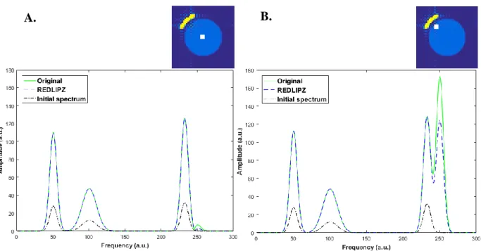
Figure 2. PSF of an object point� situated in the center of a voxel (A) showing the absence of voxel bleeding and another object located at the edge of the voxel (B) with substantial signal leaking. Each point corresponds to the center of each voxel10. PSF before (C) and after apodization using a Hamming function (D) showing the trade-off between side lobes suppression and the increase in effective voxel size9.

The PSF is usually described as a sinc function with a broadened main peak and side lobes9. The full width at half maximum (FWHM) of the main peak corresponds to the effective voxel size. For a 2D MRSI grid, the effective voxel size is 18.5% larger than the nominal voxel size9. Also, the shape and size of the object and its relative position to the points of the MRSI grid influences how the PSF will contribute to adjacent voxels. The contribution can be positive or negative and it decreases with the distance from the origin of the PSF. If the point source is located in the center of the voxel, the side lobes of the PSF will zero cross in the center of the adjacent voxels. This means that the positive and negative contributions will cancel out and the net signal is zero and, therefore, no contamination is observed. However, when the source of the signal is in the edge of the voxel there is an offset. As a result, the net signal is non-zero and a significant contamination in the adjacent voxels is observed (see Figure 2: A and B). The contamination effect is larger for water/lipid signals which, due to their higher concentrations, have stronger signals. Thus, leading to substantial contamination even in far voxels in the center of the brain, distorting the metabolite information9,10,12.

One of the adjustments to reduce the voxel bleeding is increasing k-space sampling and use more phase-encoding steps which require longer acquisition times. As an alternative, a simple way that improves the PSF while keeping short scan times is the application of k-space filters that allow the suppression of the side lobes by weighting the samples through a multiplication with an apodization function (cosine, Hamming or Hanning filters)8–10,27. However, k-space filtering results in an increase of the FWHM, which means larger effective voxel size and decreased effective resolution9,10,12.

(18)

6

2.4. Water suppression

Metabolite concentrations in the human body are much lower than those of lipids and, especially, unbound water. Thus, the sensitivity of MRS for the detection of these metabolites is much less. To overcome this problem, larger voxels (to increase SNR) or higher magnetic fields can be used. Moreover, water and lipid signals are orders of magnitude higher than those of metabolites of interest, contaminating the spectra. Thus, water/lipid signals can overwhelm those of the metabolites: even minimal residual water/lipid signal will distort metabolic information, hampering the metabolite detection and quantification. For this reason, water suppression is required.

Several water suppression techniques exist, with the most common being chemical-shift selective water suppression (CHESS)28 and variable pulse power and optimized relaxation delays (VAPOR)29. CHESS is a frequency selective excitation method that pre-saturates the water signal without perturbing the metabolite resonances using frequency selective RF pulses. VAPOR is a CHESS-based method: the flip angles of succeeding CHESS pulses and the inter-pulse delay were optimized (see Figure 3) making this method less sensitive to T1 and B1 inhomogeneity. Although CHESS is more sensitive to T1 and B1

inhomogeneity (resulting in less efficient water suppression) it allows shorter repetition times than VAPOR8–10,30.

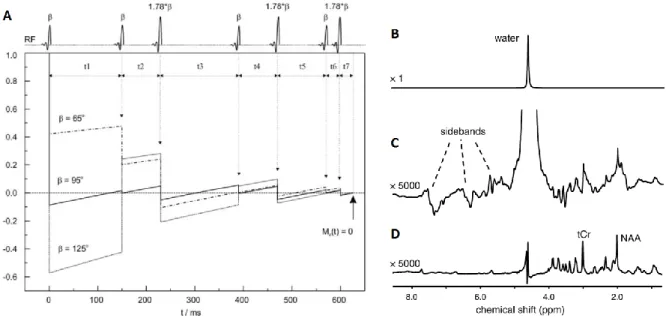
Figure 3. Scheme representing a VAPOR sequence� including seven CHESS water suppression pulses with optimized flip angles and timing (A) showing the water longitudinal magnetization (Mz) time dependence for three different nominal flip angles29. 1H-MRS spectrum in vivo of rat brain dominated by the water resonance (B) showing the low metabolite signals hidden by the water sidebands (C) representing the importance of water suppression techniques (D)9_.

(19)

7

2.5. Lipid suppression

MRSI is hindered by the presence of a strong lipid signal arising from outside of the brain (skull and scalp). Furthermore, these regions typically have a distorted magnetic field due to differences in susceptibility at air-tissue interfaces, especially around the temporal and frontal lobes (auditory and nasal canals). Consequently, water and lipid signals can be frequency shifted in these regions which makes the water and lipid suppression more difficult.

Several techniques for lipids suppression exist and are described as follows: Outer-volume suppression (OVS) uses slice-selective saturation slabs that excite the lipid regions outside the brain followed by crusher gradients that dephase the signal from these regions9; Frequency selective inversion recovery is identical to common inversion-recovery techniques and considers the chemical shift and the differences in T1 values to suppress the lipids.

However, even though these methods provide effective artifact removal, the lipid saturation or nulling without interference with metabolite resonances is still a problem. All those methods require additional RF pulses, gradient crushers and delays, which increase power deposition, duration and complexity of MRSI pulse sequences9,10,23–25,31,32.

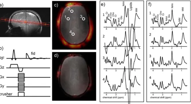
Figure 4. Example of 1H-MRSI in vivo data acquisition using a so-called crusher coil�. A transverse slice (A) in the brain acquired using a slice selective excitation, phase encoding and a crusher coil for outer volume suppression (B). Without the crusher coil, there are extra-cranial high lipid signals present (C) and the spectra contain large lipid contamination (E). When using the crusher coil the strong lipid signals is greatly suppressed (D) and the spectra show a reduction of the lipid contamination (F)31.

(20)

8

A new method for efficient lipids suppression, presented in Figure 4, is an actively switchable crusher coil that uses surface spoiling gradients to create a local distortion of the B0 magnetic field destroying the phase coherence of the skin and skull lipids. It allows

simpler sequences, improving the sampling efficiency, SNR and coverage of high resolution in short scan time. Dephasing of the signal can be incorporated in almost any sequence as it only requires a short pulse of the coil and no RF pulses or delays31.

2.6. Data post-processing techniques

There are several post-processing methods that can be applied to the MRSI data to improve the appearance of the spectra before spectral quantification algorithms are applied8,9. By manipulating the FID, it is possible to improve different aspects of the spectra such as the line width, line shape, baseline, frequency shifts and phasing.

Direct current (DC) offset correction involves a subtraction of a mean value from each point in the FID and allows the correction of spurious resonances at the center of the spectrum. Zero-filling is the extension of the FID with zeroes in order to increase the digital resolution of the spectra and to produce a better line shape representation, as shown in Figure 5. This brings us to truncation artifacts that are characterized by ripples or wiggles which occur in the spectra when the FID does not decay to zero in the end of the acquisition and zero-filling is applied18,33.

To remove truncation artifacts apodization can be applied which is a simple multiplication of the FID with a filter function, i.e. time domain filtering, creating a smooth decay to zero and removing the truncation discontinuity. The most common functions are exponential multiplication and Lorentz to Gaussian transform. The exponential weighting of the FID improves the SNR by attenuating signals in the end of the FID but increases the line width, i.e. trading resolution for sensitivity. The Lorentz-Gaussian filtering converts the Lorentzian into a Gaussian line shape, approaching the baseline faster within a narrower frequency range simplifying the fit of overlapping resonances9,18,33.

The spectra appearance depends on the phase of the signal at time zero. If at the start of the real part of the FID the value is not the maximum, then the signal is phase shifted. This shift is called a zero-order or frequency independent phase correction as it is the same for all resonances. Also, if the time domain acquisition has a delay it will cause a first-order or frequency dependent phase error in the spectrum characterized by the baseline distortions (such as shift of the spectrum, above or below the origin, or low frequency oscillations). To phase the spectrum correctly, a combination of zero and first order phase corrections should be applied18,33.

Eddy currents are caused by rapid switching of the gradients which lead to time-dependent magnetic fields offsets, causing a distortion of the main magnetic field and affecting the spectrum resonances. It can be corrected by acquiring a reference water scan and applying the opposite phase modulation of the frequency variations in the water signal to the metabolite spectrum9.

(21)

9

To remove water residuals that result from incomplete water suppression, one of the best and most reliable methods available is via Hankel-Lanczos single value decomposition (HLSVD) filter30,34 which allows the subtraction of the reconstructed water signal from the FID (see Figure 5)9,33.

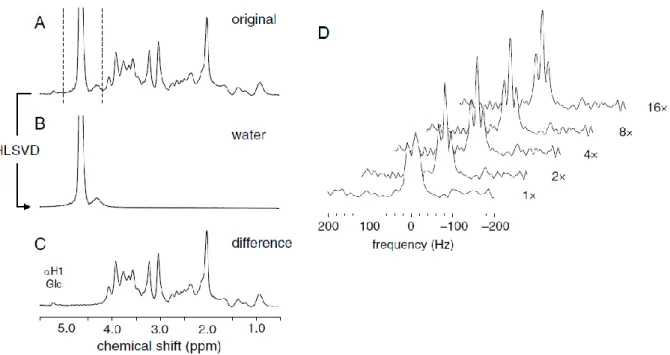
Figure 5. Residual water removal using the HLSVD algorithm in a 1H-MRS spectrum� (A) by subtraction of the calculated water spectrum with the HLSVD (B) for the frequency range indicated with the dashed lines. The resultant spectrum after subtraction (C). The effect of the zero-filling in the resolution of the spectrum shows that after zero-filling with a power of 2 is enough to distinguish the triplet resonance (D)9.

2.7. Current solutions

A study proposes35 the subtraction of lipid resonances after FT reconstruction and line fitting. However, it demonstrates some limitations as the line fitting is not able to separate metabolite resonances from the highly contaminating lipid signal. An implementation of the Papoulis-Gerchberg (PG) algorithm23 reconstructs the lipid region (band-limited signal) increasing the k-space sampling by extrapolation and, thus, reducing the Gibbs ringing effect, as shown in Figure 6. However, as more intense lipid signals are present the sensitivity to motion increases.

A similar approach36 with dual k-space sampling using two echo-planar spectroscopic imaging (EPSI) measurements was also investigated with no further improvements except its lower sensitivity to motion artifacts. Another study25 combines two different approaches, a dual-density k-space sampling37–39 and a lipid-basis cost40. The dual-density approach takes advantage of the high SNR of the lipids to suppress the ringing artifacts using high-resolution lipid maps. The second approach includes the fact that metabolite and lipid spectra are approximately orthogonal, and searches for disperse metabolite spectra when projected onto lipid-basis functions. Both these methods need longer acquisition time which is inherent to the higher sampling of the k-space.

(22)

10

A method12 that was recently introduced applies the sensitivity encoding acceleration technique with spatial over discretization to reconstruct parallel MRSI data. By minimizing the deviation of the spatial response function (SRF) with a target SRF chosen beforehand, it allows effective SRF side lobes suppression while avoiding an excessive increase of the effective voxel size. However, there is some susceptibility to sensitivity calibration errors, motion artifacts and remaining B0 fluctuations after shimming.

Figure 6. Example of Papoulis-Gerchberg extrapolation algorithm�. Spectra from voxels across the brain using zero-fill FT reconstruction (A) and Papoulis-Gerchberg extrapolation (B). The reduction of lipid contamination is evident when using the PG extrapolation (B) and the lipid signal also becomes concentrated in a narrower region23.

2.8. Objective

MRSI suffers from an effect referred to as “voxel bleeding”, a consequence of the inherent low spatial resolution and limited k-space sampling with zero-filling. This effect represents a problem since extra-cranial lipids signals are orders or magnitude higher than those of metabolites. They contaminate the metabolite spectrum and distort information, leading to incorrect detection and quantification.

The goal of this study was to develop a post-processing method to reduce high lipid signal emanating from extra-cerebral tissue (skin/skull) which contaminate the brain tissue spectra. Using prior knowledge of the PSF, we attempt to improve the quantification of metabolite concentrations.

(23)

11

3. Materials and methods

3.1. Data acquisition

2D MRSI data of the brain was acquired using a 7 Tesla MR System (Achieva, Philips Healthcare, Cleveland, Ohio, USA) in combination with a 3channel receiver array and a 2-channel volume transmit head coil (Nova Medical, Wilmington, MA). An image based 2nd order shimming was performed to minimize B0 inhomogeneity17. An in-house developed

crusher coil31 placed inside the head coil provided fast and efficient extra-cranial lipid suppression. The crusher coil consists of a circuit placed around the head which is pulsed with a drive current producing a local and inhomogeneous magnetic field that dephase signals from the skull. The crusher coil was activated for 1.8 ms during the echo time (TE). Reconstruction of spectroscopic data was performed by the scanner.

Phantom data was acquired to test and validate our approach. Two phantoms were used, one containing water (water phantom containing metabolite signal) with acetate, ethanol and phosphate (H3PO4), and the other containing sunflower oil (lipids phantom). The phantom

CSI datasets include a water reference scan without water suppression and a metabolite scan with CHESS water suppression (both scans were acquired with both phantoms and then repeated only with the water phantom). These were acquired using a pulse-acquire sequence and CHESS water suppression [FOV = 220 x 220 mm2, voxel size = 5 x 5 x 10 mm3, reconstruction matrix = 44 x 44, TR = 300 ms, TE = 2.5 ms, CHESS pulse bandwidth = 300 Hz, number of samples = 512, bandwidth = 4000 Hz, spectral resolution = 7.8 Hz, total acquisition time = 7min36s]. The phantom data were reconstructed with and without a k-space cosine apodization filter which is typically used by the scanner to reduce the PSF side lobes and, consequently, the contamination in the MRSI data.

In vivo CSI datasets of the brain (a water reference scan without water suppression and

a metabolite scan with CHESS water suppression) were also acquired from a healthy volunteer using the same sequence with the following imaging parameters [FOV = 220 x 220 mm2, voxel size = 5 x 5 x 10 mm3, reconstruction matrix = 44 x 44, TR = 300 ms, TE = 2.5 ms, CHESS pulse bandwidth = 300 Hz, number of samples = 512, bandwidth = 3000 Hz, spectral resolution = 11.7 Hz, total acquisition time = 7min36s]. This dataset was reconstructed with the k-space cosine apodization filter. For an anatomical reference and segmentation of the brain, a 3D T1 weighted scan was also acquired using the Magnetic

Prepared Rapid Acquisition Gradient-Echo (MPRAGE) sequence41 [FA = 6˚, TR = 8 ms, TE = 2.9 ms, slices = 220, voxel size = 1 x 1 x 1 mm3]. To reduce the B1 receive inhomogeneity,

these T1 weighted were divided by a proton density (PD) weighted image [TR = 8 ms, TE =

1.72 ms, FA = 5˚, voxel size = 2 x 2 x 2 mm3

(24)

12

3.2. Data post-processing

All data processing was performed using a commercial software package (MATLAB 2014b, The MathWorks Inc., Natick, MA, 2000). A LC Model-based Matlab script (in-house modified version of NMR Wizard, R.A. de Graaf, 1999) was used to process the data (Appendix A). LC-Model42 is an automatic method to analyze in vivo spectra as a Linear Combination of Model in vitro spectra basis. The residual water resonance and sidebands were removed from the metabolite spectra by subtraction of the water fit of the reference water spectra. To remove the remaining water residuals, the HLSVD filter34 was applied. A software package43 (jMRUI 4.0, http://www.jmrui.eu/) for time-domain analysis of MRS data was used to phase the spectra (Appendix B). B1 correction was not performed.

3.3. REDuction of LIPid contamination with Zero-padding (REDLIPZ)

A two-dimensional FT was applied to the original image, referred to as Original, to return to the spatial frequency domain, i.e. the k-space. The total resulting k-space was retained and zero-padded to twice the size of the original k-space. The modified k-space was named as

Zero-padded k-space. Subsequently, a two-dimensional inverse FT was applied to the

modified k-space to reconstruct the data, generating an interpolated image, named as

Interpolated, with two times the resolution of the Original image.

Afterwards, a mask of the lipid signal region was selected on the Interpolated image, named Mask. The mask ensures that the calculated PSF knowledge would only include the signal contamination from the lipid signals outside the brain. For the phantom data, the mask was created using the Matlab function imellipse allowing the selection of an elliptical region on an image. For the in vivo data, the mask of the skull was defined with the same Matlab function but using a segmented T1 weighted image as an anatomical reference of the brain to

exclude the brain region. A two-dimensional FT was applied to the mask to return to the space. The center portion of the resulting space (corresponding to the original size of the k-space before zero-padding) was retained and a two-dimensional inverse FT was applied, causing the voxel bleeding effect. This resulting PSF knowledge included the signals leaking from high lipid regions (see Figure 7: PSF). To remove signal leakage, the PSF image was subtracted from the Original image producing the clean MRS image (Clean) with less lipid contamination (see Appendix C).

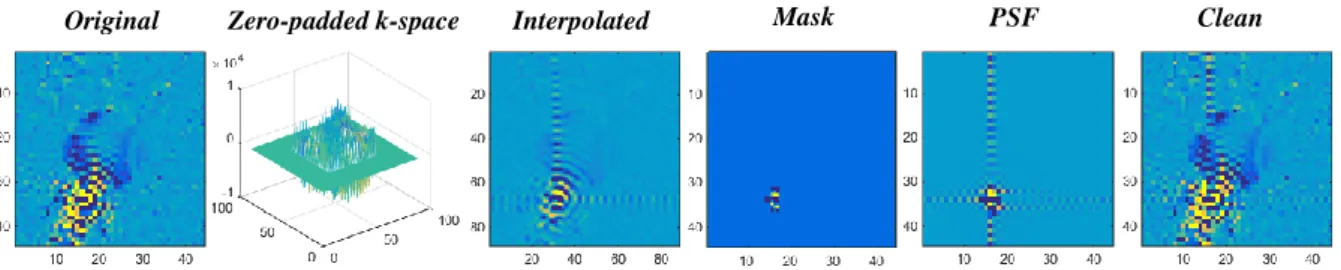
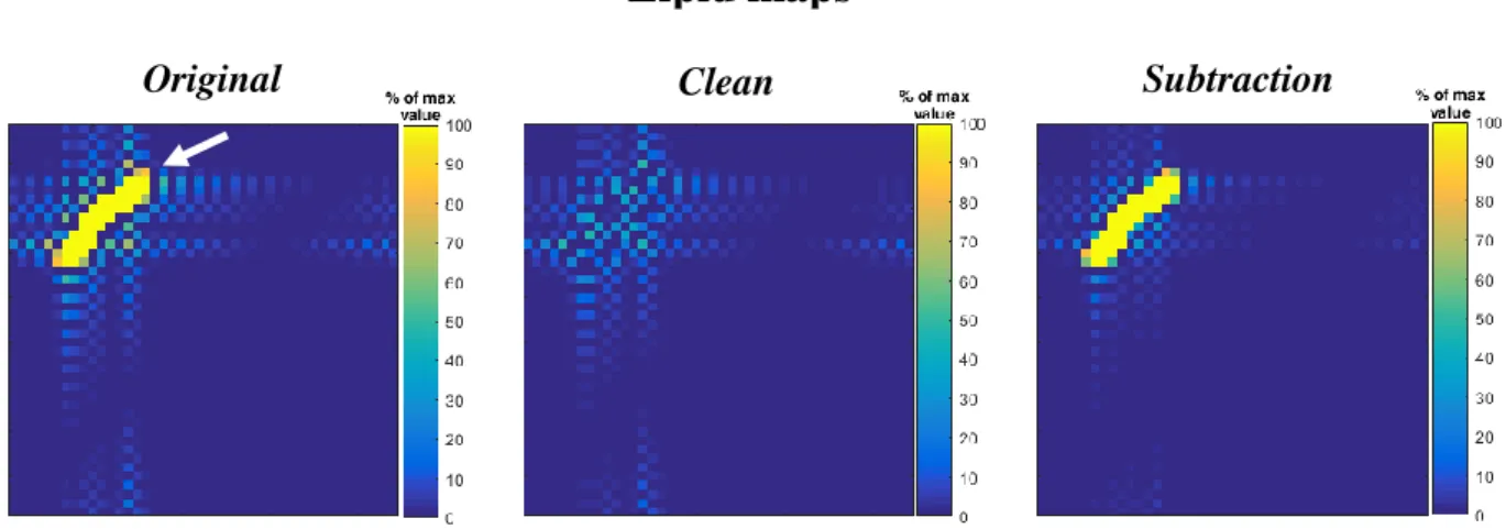
Figure 7. Representative scheme of the REDLIPZ method�. MRSI images for the lipid resonance showing from left to right: the original data (Original), the interpolated image with ringing artifacts (Interpolated), the lipids mask (Mask), the voxel bleeding effect of the lipid mask (PSF) and, finally, the resulting image from the subtraction (Clean).

(25)

13

3.4. Simulations

Simulations using artificially generated 2D MRSI data of the brain were performed with the purposes of testing our method and better understanding its outcomes. The simulation (Appendix D) started by generating the MRSI data of the brain. Spectral data with 300 sample points was produced using Gaussians to simulate both metabolite and lipid resonances. Three peaks with low amplitude were used to represent the metabolites, named A, B and C, and one peak with an amplitude two orders of magnitude higher was used to simulate the lipid resonance (Figure 8: left panel). Also, two different geometrical regions, a circle and a circumference, were defined in the MRSI grid (matrix of 88x88) to represent the brain and the skull, respectively. The region representing the skull was not a complete sphere-like region because the intention was to simulate an incomplete suppressed lipid region. So, for that reason, only a quarter of the “skull” was included (see Figure 8: right panel).

With the spectral data simulated and the regions defined, the next step was to assign different spectra to the corresponding regions. Spectra including only peaks resembling the metabolite information were assigned to the region representing the brain and spectra including only the high peak representing high lipid signals was ascribed to the skull region. With these steps completed, an ideal 2D MRSI data of the brain was produced. However, our interest was to simulate the real conditions in MRSI data, i.e. the low spatial resolution and the limited k-space sampling with zero-filling, and resultant voxel bleeding artifact. To do this, a zero-filling technique was applied to the data as explained below.

Figure 8. Simulated MRSI data of the brain�. Simulated spectral data including three different peaks representing the metabolites A, B and C resonances and one peak with higher amplitude representing the high lipid resonance (Simulated

spectra). Image with the different regions representing the brain (main circle) and part of the skull (Regions mask). The

metabolite spectrum was assigned to the brain region and the lipid one to the skull region.

The zero-filling started with a two-dimensional FT that was applied to the original MRSI data to return to the k-space. The center portion of the k-space, which is half of the original size (44x44), was retained and the remaining outer portion was zero-filled up to the original size of the k-space. Thus, the size of the k-space before and after the zero-filling was the same (88x88) and the only difference was between the outer portion that was replaced

ppm Regions mask Simulated spectra A m p li tu d e (a .u .)

(26)

14

with zeroes. A two-dimensional inverse FT was then applied to the zero-filled k-space to reconstruct the MRSI data which included the Gibbs ringing artefact. Finally, we attempted to clean up the data using the REDLIPZ method to see if the original data quality could be restored.

Figure 9. Ideal MRSI simulated data (Ideal data) and more realistic MRSI data (Zero-filled data) � after zero-filling of the k-space showing the resulting contamination effect commonly observed in real MRSI data.

3.5. Experiments

Metabolite and lipid maps were calculated from the simulated data by plotting the magnitude of respective peak heights at each voxel location. The maps before (Original) and after (Clean) the application of the method were normalized to the maximum of the Original. Data was expressed as a scaled percentage of the maximum signal value. Individual spectra for two voxels selected from regions with different levels of contamination were analyzed.

For both phantom and in vivo data, the metabolite and lipid maps were calculated from the absolute values of the spectra by integration of the area under the resonance peak. The frequency ranges which were used for integration and finding the peak height in the phantom data were: 1.82-1.96 ppm for acetate and 0.81-1.31 ppm for lipid; and in the in vivo data were: 3.23-3.33 ppm for choline and 1.24-1.32 ppm for lipid. The ratio maps between metabolite and the lipid peak heights were also calculated. All the maps before (Original) and after (Clean) the application of the methods were normalized with respect to the maximum of the

Original and scaled in percentage of the maximum signal value. The data was also used to

produce MRSI data with lower resolution, using the same zero-filling method used in the simulations, and the respective maps were generated. The spectra of two voxels in regions with different levels of voxel bleeding were also evaluated.

For phantom data, the maps and spectra of the data acquired with and without the cosine apodization filter were assessed. Also, a comparison between the reference scan (only water phantom) and the metabolite scan (both water and lipid phantom) was performed for the phantom data without the apodization filter. Here, the ratios between the peaks of acetate and ethanol were compared.

Zero-filled data Ideal data

(27)

15

3.6. Secondary experiments

An experiment was performed to optimize the speed of the pre-processing of the MRSI data used in this work. Not all the voxels of the acquired MSRI data contain relevant information to be analyzed. A lot of time is spent on processing of those voxels without important data for the spectral analysis. The acquired MRSI data had a matrix size of 44x44 which corresponds to 1936 voxels to be evaluated. However, a great number of voxels can be excluded, considering that only approximately 60% of the voxels correspond to the head (brain and skull) and only a portion of those actually have good quality spectral data to be analyzed. Only a small part of the whole data has sufficient quality to be assessed but, still, the whole matrix was being processed with NMR wizard. The processing of the entire matrix is time-consuming and this could be avoided by previously excluding non-relevant voxels. To make this process more efficient and faster some selection criteria were used: only voxels that had been included in a brain mask and had a fitted water area above 50% of the average water area, were processed.

(28)

16

4. Results

4.1. Simulations

By comparing the lipid maps before and after the implementation of the REDLIPZ it is possible to observe an evident reduction of the lipid signal (Figure 10: left panel, white arrow). We can also see that after the application of the method some ringing artifacts are still present.

Figure 10. Lipid maps of the simulated MRSI data� before (Original) and after the application of the REDLIPZ method (Clean) showing evident reduction of the high lipid signal indicated by the arrow in the Original image.

The same comparison for the metabolite (Figure 8: metabolite C) maps show presence of the metabolite signal in the simulated skull region, as shown in Figure 11. However, this should not be possible since no metabolite resonance was assigned to that region. After applying the method there is a clearly reduction of the metabolite signal in the lipid region, but some ringing artifacts are remaining.

Lipid maps

(29)

17

Figure 11. Metabolite maps of the simulated MRSI data� before (Original) and after the implementation of the REDLIPZ method (Clean) show reduction of the lipid signal contamination indicated by the arrow in the Original image.

The observed reduction of the lipid signal in the previous metabolite and lipid maps can also be seen in the spectra of two different voxels with different levels of lipid contamination (see Figure 12).

Figure 12. Spectra of the simulated MRSI data� before and after implementation of the REDLIPZ method of a voxel from a region with low contamination (A) and another one voxel from a region with higher contamination (B). In both voxels is possible to see the lipid peak reduction pointed by the arrows. The position of the voxels is illustrated by the white squares on the maps on top.

Metabolite maps

Original Clean

(30)

18

4.2. REDLIPZ

4.2.1. Phantom data without apodization filter

The position of the phantoms is illustrated in Figure 13.

Figure 13. Water and lipid phantoms positions� are shown.

For the phantom data acquired without the apodization filter, a comparison between the lipid maps before and after the implementation of the REDLIPZ method was done (see Figure 14). It is possible to see some reduction of the high lipid signal indicated by the white arrow in the Original image.

Figure 14. Lipid maps of the phantom data without apodization filter� before (Original) and after the application of the

REDLIPZ method (Clean). Some reduction of the lipid signal can be observed which is pointed by the arrow in the Original

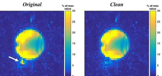
image. Water Lipid Clean Original

Lipid maps

(31)

19

Through a closer observation of the lipid maps (Figure 15) it is possible to understand that even though there is some reduction of the lipid signal, the reduction of the ringing artifacts on the water phantom in the region with high contamination is insignificant.

Figure 15. ROI (lipid phantom region and the water phantom region with higher contamination) of the lipid maps of the

phantom data without apodization filter� before (Original), after the application of the REDLIPZ method (Clean) and the subtracted signal (PSF).

The same comparison between the acetate maps was made, as shown in Figure 16. A reduction of the acetate signal can be observed. The small yellow spot pointed by the arrow in the Original image, disappears after the application of the method. This spot would suggest presence of acetate in the lipid region which is not possible since the lipid phantom has no acetate. Moreover, an inhomogeneous signal inside the phantom can be seen.

Figure 16. Acetate maps of the phantom data without apodization filter� before (Original) and after the implementation of the

REDLIPZ method (Clean). It is possible to see some reduction of unexpected acetate signal, indicated by the arrow in the Original image.

In the spectra shown in Figure 17 it is possible to observe the baseline distortions caused by the high lipid signal and the consequent increase in the values of the other resonances. The baseline distortion causes an increase of two orders of magnitude on the values in the acetate integration range.

Clean

Original PSF

(32)

20

Figure 17. Absolute values of a spectrum from a voxel in the lipid phantom region� before and after the application of the

REDLIPZ method showing the baseline distortion caused by the high lipid signal.

No perceptible changes can be observed in the ratio maps between acetate and lipid peaks presented in Figure 18. However, an increase in the region with higher lipid contamination was expected.

Figure 18. Maps of the ratio between acetate and lipid peaks of the phantom data without apodization filter� before (Original) and after the application of the REDLIPZ method (Clean) with any perceptible changes.

The comparisons in Figure 19 and Figure 20 show that the peak height percentage differences are lower than 0.3% for acetate and 3.1% for ethanol in both voxels. Within the example voxel having high lipid contamination, the reduction in the lipid signal is 10.3%. The changes in metabolites are minimal. The observations are in agreement with the insignificant changes observed in the acetate maps and the detected reduction in the lipid maps. The comparison between the reference and the processed spectra show that the ratio between acetate and ethanol is 4% lower in the voxel with low contamination, and 13% lower in the voxel with high contamination.

(33)

21

Figure 19. Comparison using peak height % difference and peak height ratio between phantom spectra before and after

processing with the REDLIPZ method (A) of a voxel from a region in the phantom with low lipid contamination�. The position of the voxel is indicated by the white square on the map on top. Peak height ratios of a reference spectra (water phantom only) and the processed spectra (water and lipid phantoms) from the same voxel (B).

Figure 20. Comparison using peak height % difference and peak height ratio between phantom spectra before and after

processing with the REDLIPZ method (A) of a voxel from a region in the phantom with high lipid contamination�. The position of the voxel is indicated by the white square on the map on top. Peak height ratios of a reference spectra (water phantom only) and the processed spectra (water and lipid phantoms) from the same voxel (B).

A B