See discussions, stats, and author profiles for this publication at: https://www.researchgate.net/publication/5852562
Computational and Statistical Methodologies for ORFeome Primary Structure Analysis
Article in Methods in Molecular Biology · February 2007
DOI: 10.1007/978-1-59745-514-5_28 · Source: PubMed
CITATIONS 3
READS 116
5 authors, including:
Some of the authors of this publication are also working on these related projects:
Pulmonary Rehabilitation Innovation and Microbiota in Exacerbations of COPD - PRIME View project
Pulmonary Rehabilitation Innovation and Microbiota in Exacerbations of COPD - PRIMEView project Gabriela Moura University of Aveiro 143 PUBLICATIONS 1,136 CITATIONS SEE PROFILE Miguel Pinheiro University of Aveiro 76 PUBLICATIONS 883 CITATIONS SEE PROFILE Adelaide Freitas University of Aveiro 39 PUBLICATIONS 264 CITATIONS SEE PROFILE
José Luís Oliveira
University of Aveiro
223 PUBLICATIONS 1,402 CITATIONS SEE PROFILE
Computational and Statistical Methodologies for
ORFeome Primary Structure Analysis
Gabriela Moura1, Miguel Pinheiro2, Adelaide Valente Freitas3, José Luís Oliveira2 and Manuel A. S. Santos1*.
1
Department of Biology and CESAM, 2DET/IEETA, 3Department of Mathematics. University of Aveiro, 3810-193 Aveiro. Portugal.
Corresponding author. Manuel A. S. Santos Department of Biology University of Aveiro 3810-193 Aveiro Portugal [email protected]
Running title: Large scale codon context analysis.
Keywords: Genome, ORFeome, gene primary structure, codon context, codon usage.
Abstract
Codon usage and context are biased in open reading frames (ORFs) of most genomes. Codon usage is largely influenced by biased genome G+C pressure, in particular in prokaryotes, but the general rules that govern the evolution of codon context remain largely elusive. In order to shed new light into this question we have developed computational, statistical and graphical tools for analysis of codon context on an ORFeome wide scale. In here, we describe these methodologies in detail and show how they can be used for analysis of ORFs of any genome sequenced.
1. Introduction
Genome sequencing is opening unprecedented ways for understanding the primary structure of open reading frames on a global scale and the evolutionary forces that shape them (ORFeome analysis). Codon usage has been intensively studied in many organisms and one already has a relatively good understanding of the structural and functional constraints that shape its evolution. Conversely, other important features, such as codon context (two neighbor codons), tandem codon repeats and amino acid composition have not been so well studied and we are still far from understanding their importance for gene stability, mRNA decoding efficiency and accuracy (1-5). Codon context is rather interesting because it is biased and has an important impact on tRNA decoding accuracy but the rules that define good and bad context of neighbor codons are not yet understood. Additionally, it is not yet clear whether codon context is used to regulate speed of mRNA translation, whether it influences ribosome drop out during elongation and how genes with bad codon context are translated under physiological stress. Considering that mRNA decoding accuracy is critical to ensure correct flow of
genetic information from DNA to protein, understanding those rules is likely to provide new insight on the constraints imposed by the mRNA translation machinery on gene evolution. More importantly, codon context rules would allow one to redesign the open reading frames of genes for optimal expression in heterologous hosts (6, 7). This is of practical relevance since previous studies carried out in our laboratory have shown that codon context is species specific and consequently heterologous genes do not have the most appropriate context for translation by the host translational machinery.
Traditional methods used for codon usage and context analysis do not provide user-friendly tools to carry out detailed gene primary structure analysis on a genomic scale. Codon usage tables, using absolute metric, are available in public databases for any sequenced gene or genome (http://www.kazusa.or.jp/codon/) and free-ware software for multivariate analysis (correspondence analysis) of codon and amino acid usage is also readily available (http://bioweb.pasteur.fr/seqanal/interfaces/codonw.html). However sophisticated statistical and data visualization tools are clearly lacking. In order to study context bias in complete ORFeomes, we have constructed a bioinformation system herein named ANACONDA, which imports FASTA files, and performs a series of analyses that permit elucidating how codons are associated in consecutive pairs, either in coding sequences or in non-coding regions. This methodology allows to differentiate general biases imposed by general rules of genome evolution, which are related to DNA replication biases (8-11), from biases imposed by the mRNA translational machinery (1, 2, 12-18). In here, we describe the architecture of ANACONDA and how it can be used to analyse gene primary structure on an ORFeome scale.
2. Materials
ANACONDA is a software package specially developed for the study of genes’ primary structure. It uses open reading frame sequences (ORFeomes) downloaded from public databases in FASTA format and it uses a set of statistical and visualization methods to reveal information about codon context, codon usage and nucleotide repeats within open reading frames. The general features of ANACONDA are described below.
1. Software - the ANACONDA software was developed in C++ language with Microsoft Foundation Class (MFC), it runs on MS Windows, and it can be downloaded for non-commercial usage from the site: http://www.bio.ua.pt/genomica/lab.
2. Requirements – Windows (98/Me, NT 4.0 SP6, 2000 or XP), Processor - 600 MHz Intel Pentium III or equivalent, Memory - 128 MB of RAM (256 MB or more recommended). Disk space available - 100 MB, Minimum resolution - 800 x 600 (1024 x 768 or higher recommended).
3. Data - The genomes files processed by the ANACONDA must be in the FASTA format.
4. Parameters - The reference values of Relative Synonymous Codon Usage are necessary for the calculation of the Codon Adaptation Index (CAI) (19). This data must be introduced manually. In the current version, the ANACONDA database includes RSCU values for Candida albicans, Saccharomyces cerevisiae and
3. Methods
In this section, we describe the main tools of ANACONDA which are divided into four main parts, namely: i) uploading and validation of DNA sequence data into the local database; ii) building ORFeome maps for two-codon context bias; iii) visualization and analysis of the two-codon context biases in individual sequences and iv) comparison of the codon biases across multiple ORFeomes. Also, and taking advantage of the fact that ANACONDA interprets DNA sequences as sequences of trinucleotides (codons), several tools regarding codon usage analysis have been implemented, as explained below.
3.1 Statistics methods
ANACONDA uses contingency tables as the basic statistical methodology and identifies preferred and rejected codon pairs of an ORFeome through the analysis of adjusted residuals values of the contingency tables. The following list highlights the main statistical procedures performed by the software.
1. ANACONDA uploads ORFeome sequences from any genome and reads them in the 5´to 3´direction fixing each codon (ribosomal P-site) and memorizing its neighbour codons (E-site codon and A-site codon).
2. The data extracted by ANACONDA is then transferred to a 64x61 contingency table with two categorical variables: A and B (Table 1). Variable A represents the 64 possible codons located in the ribosome P-site and variable B represent the following codon (A-site codon) for each observed codon pair in the ORFeome (See Note 1).
3. ANACONDA then calculates the value of the Pearson’s chi-squared statistic and the adjusted Pearson residual values. Pearson’s statistic represents a global measure of the difference between observed and expected codon frequencies (20).
4. If the hypothesis of independence between the variables Ai and Bj is rejected, i.e. between contiguous codons, ANACONDA determines the contributions of each 64x61 codon pairs to Pearson's statistic value computing the adjusted residual values (21). 5. The obtained adjusted residual value, for each pair, is then converted into a colour coded scale and the information is displayed in a 64x61 codon context map, where green represents positive adjusted residual values greater than +5 (herein called preferred codon pairs) and the red represents negative adjusted residual values lower than -5 (herein called rejected codon pairs). The adjusted residual values that fall within the interval of -5 to +5 correspond to codon contexts that do not contribute to context bias for confidence levels greater than 99% (21) and are shown in black.
3.2 Uploading of raw data
1. Reading sequences. The ANACONDA reads any genome sequence that has been
stored in FASTA format (See Note 2). The length of each ORF and the number of ORFs in a single file are virtually unlimited. Several files can be opened simultaneously. The imported data, coming from single or multiple files, is classified in a hierarchical tree view, considering three different information levels: species, chromosomes and genes.
2. Validation of open reading frames (ORFs). When scanning the ORFeome,
ANACONDA filters pseudogenes or erroneous ORFs resulting from deficient annotation and/or sequencing errors. A number of quality control rules are defined to
allow for filtering the ORFeome. For example, very small ORFs (usually below 100 nucleotides in length), ORFs whose nucleotide sequences are not multiple of 3, ORFs without stop codons or ORFs with premature stops, are excluded. Each rule can be individually activated according to the user needs. For instance, if the goal is the analysis of all coding and non-coding sequences, all validation controls can be de-activated before opening the files.
3. Data processing (Quantification). The imported sequences are then processed
according to the statistic methodology that reveals the irregularities in the codon context along the genome. In this phase, sequence processing can be avoided if the aim is to apply data from a previous statistical analysis to a current analysis. Also, sequences with particular characteristics, or groups of genes can be excluded (at the beginning or at the end) from quantification. The length of the codon context can also be modified, i.e., instead of analyzing codon-pairs, triplets of codons or long range context effects can be studied.
4. Evaluation of the sequences quality. Once the raw data is processed, ANACONDA
generates a report showing rejected ORFs and a small description of the rejection. Valid ORFs, using particular set of filters, are shown on a specific menu “Valid Tab” on the left panel of the screen (Fig 1). ORFs excluded from analysis appear in the “Rejected Tab” of the same panel. This allows simple visual inspection of all sequences present in the original FASTA files.
3.3 Working with genomic maps of two-codon context
1. Creating an ORFeome context map. After processing of valid sequences, an entry
window of ANACONDA (Fig 1). This panel follows a hierarchical architecture with individual sequences, chromosomes and genomes. Clicking on each group of ORFs, i.e. chromosome or genome, will open the respective map for two-codon context bias on the right panel of ANACONDA’s main window (See Note 3).
2. Interpretation of genomic maps. The map represents the bias detected for
two-codon contexts in the selected set of ORFs. The bias is given by a color scale in which red stands for rejected and green stands for preferred codon pairs, in relation to what would be expected in a random basis. Each possible combination of two codons, i.e. each possible context, is represented by one small square of the map and identified by the codon of the line and the codon of the column to which the small square belongs (See Note 4).
3. Data from individual contexts. In order to facilitate interpretation and analysis of
genomic maps, the two-codon contexts can be selected with the cursor and individual information from them will be displayed in the status bar of the software’s window. These include: i) number of genes used to calculate the bias; ii) full name of both axes of the map; iii) residual value for that context; iv) occurrence for that codon pair in the genome under analysis.
4. Additional data. Apart from the data directly included in the map, ANACONDA
produces additional data about the sequences analysed, namely:
4.1. Codon counting and rare codons. The frequency of each codon is plotted
in a graph, for a chosen set of sequences, either for one chromosome or for the entire genome. This can be obtained with the tool Options->Rare Codon, since it allows determination of a threshold for codon usage that automatically indicates whether a codon is rare (See Note 5). This window also presents the total number of codons present in all valid ORFs of an ORFeome.
4.2. Nucleotide counting. Codon context has been further explored focusing on
the relative frequency of each nucleotide on each position of the neighbour codon, either at the 5’ or at the 3’ sides. This information is available on dialog Options->Nucleotide
Counting that produces a graphical visualization of nucleotide neighbourhood for any
given codon.
5. Further manipulation of the map. Certain aspects of the map for two-codon context
can be altered by the user.
5.1. Colours and intervals. The colours used to represent the deviation from the
expected mean (the residuals scale) can be chosen from a colour palette on the Options menu. Also, the residual values defining the different intervals can be modified by the user.
5.2. Cluster analysis. In order to define codon context patterns both axes of the
64x61 map can be clustered (22). Additionally, columns and/or lines can be ordered alphabetically by the nucleotide at each codon position (N1, N2 or N3). This approach was implemented in response to the preliminary observation that some positions from two consecutive codons are highly correlated (23) (See Note 6).
5.3. Exporting images. The entire map or parts of it can be copied and pasted as
images into other applications (using the drag-and-drop or the edit-copy functionalities)
6. Exporting data. The numerical data that give origin to a map can be exported as an
Excel worksheet. This will include raw data and residuals data of all map layouts, i.e. 64 x 61 codons; 21 x 21 amino acids; etc, through the option File->Save Matrix.
3.4 Working with individual ORF sequences
1. Mapping ORFs. In order to detect the impact of codon context bias (as well as the
presence of rare codons) on coding sequences, ANACONDA has additional tools for sequence mapping. These can be activated by selecting individual ORFs on the hierarchical left panel of the software’s main window (Fig 2). The layout for sequence analysis (called “view gene”) will appear on the main panel and include written information about the ORF and the sequence itself, in which the codons have been coloured with the same residual colour scale of the ORFeome map. Again, passing the cursor over the sequences will highlight additional information about each selected context in the status bar of the main window. The threshold for colouring the sequences, together with the choice for mapping rare codons on them can be customized by the user at the dialog Options->View Gene.
2. Exogenous ORFs and codon optimization. In order to optimize ORF sequences for
heterologous gene expression, or for de novo gene synthesis, ANACONDA has an algorithm that colour codes the sequence of the heterologous ORF according to the codon context rules of the host expression system. For this, the user must open the heterologous ORF sequence using the “no quantification” option (See Note 7) and then re-direct the file to the genome of the host of interest (See Note 8). The display window will then show the distribution of good and bad context for that gene.
3. Additional information. Apart from the sequence information that is shown in the
gene view layout (See Note 9), the program offers additional information, obtained from individual sequences or groups of sequences, i.e. chromosomes or total ORFeomes. Selecting the Global gene information option in the View menu the available information about that particular sequence will be displayed (See Note 10). This includes codon and amino acid counting and also several indexes relevant for
codon usage characterization, such as G + C content at individual codon positions (first, second or third); the Effective Number of Codons (24); the Relative Synonymous Codon Usage (RSCU) value for each codon; and the correspondent Codon Adaptation Index (CAI) (19) (See Note 11).
4. Filters. Searching for specific ORFeome features can be performed using sub-sets of
ORFs. The sequences that comply with the imposed rules are presented in a special tab in the left panel (Filtered). The available “filters” include: i) searching for special color patterns or codon/amino acid sequences; ii) searching for runs of up to 6 rare codons; iii) looking for ORFs rich in bad contexts or rare codons; iv) finding ORFs whose G + C % is included in a chosen interval. This filter tool is very useful for studying the distribution of these variables along an entire ORFeome. It also helps finding specific sequences or ORFs with extreme values for a particular variable (See Note 12).
5. Image and data exporting. As with genomic maps, any part of the gene view layout
can be selected and copied into another application. Also, numerical data associated with filtered ORFs can be exported as Excel worksheet by clicking on the ORF set at the Tab Filtered window with the right mouse button.
3.5 Working with more than one ORFeome
1. Workspaces. ANACONDA allows the user to work with more than one ORFeome at
a time. This creates large data sets that are difficult to deal with, in particular when multiple comparisons are being performed. To overcome this problem, ANACONDA has a Workspaces interface that permits saving all data sets, thus eliminating the need of repeating ORFeome analysis manually each time one inter-ORFeome analysis is required. When relevant ORFeomes have been opened for the first time the software
creates a file of pathways that allows ANACONDA to re-open the same files at any time (See Note 13).
2. Visualization. All opened files are named as entered by the user, are represented in
the hierarchical left panel and sorted by opening order. This way, each file can be selected, “navigated”, and analysed independently as described above (See Note 14).
3. Tools for ORFeome comparison. Considering that vast number of ORFeomes can
be analyzed simultaneously by ANACONDA, we have included extra tools to allow comparative studies.
3.1. Data normalization. Since adjusted residuals are sensitive to ORFeome
size and there is a large size difference between small bacterial and eukaryotic ORFeomes the software includes an option for size normalization that allows direct comparison of all sequenced ORFeomes of the three of life (See Note 15).
3.2. Comparing maps. ORFeome maps for two-codon-context bias can be
compared in pairs using the Processing->Compare Genomes option. This tool will produce a Differential Display Map (DDM) that results from subtracting both maps cell-by-cell. DDMs can also be manipulated by the user as described for normal ORFeome maps.
3.2. Clustering. Alternatively, all opened maps can be compared in one single
display to allow detecting overall patterns of two-codon context. This can be achieved with the option Processing->Compare all genomes. When this option is selected, ANACONDA will transform the 64 x 61 maps of each opened ORFeome into one single column of 3904 lines, one for each possible codon pair. In a second step, all columns are aligned set side-by-side to allow immediate comparison of patterns. As
with all 64 x 61 maps, it is possible to rearrange this large-scale comparative map through cluster analysis of both axes to highlight major common patterns (Fig. 3).
4. Exporting data. Similarly to the 64 x 61 maps, the adjusted residuals of large-scale
comparison maps can be exported as CVS files for further mathematical analysis.
4. Notes
1. The contingency table is a 64x61 matrix. Since stop codons do not have codons on their 3´-side the three columns corresponding to these three codons are not defined. 2. For a more detailed description of FASTA format see
www.ncbi.nlm.nih.gov/BLAST/fasta.html. As an example, the complete set of ORFs from a single species can be found in a format appropriate for ANACONDA in .ffn files of GenBank (ftp://ftp.ncbi.nih.gov/genomes/). If needed, this format must be applied to other sequences before opening them with ANACONDA.
3. In most cases, data presented by this software is calculated based on the ORF or ORF set selected in the left panel of the main window. If a special set of ORFs is to be analyzed it must be formatted as a FASTA file containing the chosen ORFs and then be opened by ANACONDA at later stage.
4. In the maps of two-codon context created by ANACONDA the lines represent fixed codons as indicated on the left, while the columns correspond to codons standing on the 5’ or 3’ sides of the fixed codon, as indicated at the top of the map. The type of context (5’ or 3’ side), as well as the type of map (showing codons, amino acids or nucleotide positions), can be chosen using a drop-down menu on the top-right corner of the main window.
5. Rare codons are highlighted by a blue circle in the sequence view layout, and will be considered in future versions of ANACONDA as codons to be preferentially optimized.
6. Usually, the last position of one codon (N3) is highly correlated with the first position of the following one (N4), as seen by the formation of single colour larger squares in the maps (23).
7. By default, when opening a new set of DNA sequences the software will quantify them, i.e. will count codon pairs and calculate the adjusted residuals. However, sequences can be opened without quantification in order to be analysed with residuals calculated with other sequences. This can be achieved by simply choosing the “No quantification” option of the Processing window.
8. A sequence that has been opened with no quantification can be analysed with residual data extracted from other Orfeomes. For this, the user must select the sequence using the hierarchical left panel and click on its name with the right mouse button. Then the option “re-direct” must be selected, as well as the genome whose residual data is to be used. The sequence will then appear at the gene view layout, coloured as if it belonged to the host genome.
9. The header of the gene view layout includes: 1) the ORF name; 2) the total number of codons of that ORF; 3) the number of codons whose frequency is below the chosen threshold for rare codons; 4) the percentage of rare codons in the ORF; 5) the type of map and how data was quantified to reach the residuals used; 6) the count and the percentage of two-codon contexts whose calculated residues belong to each colour of the scale shown in the layout. Additionally, ANACONDA allows counting the total number of particular codons, as specified in the gene view options.
10. Alternatively, the same information can be obtained using the “i” button of the toolbar. Also, the option View->Gene (Nc, total GC, GC3, CAI) offers a reduced
version of the same information but in a floating window, that allows selecting
different ORFs without closing it.
11. The CAI value for the selected sequence will appear only when the RSCU data for reference genes have been typed in. This has to be done manually, choosing Add in the window for defining RSCU values of the Options->Define RSCU Values menu. Each set of RSCU values can be saved for later use. To define the RSCU values of a genome, right button click in the genome name and choose RSCU values: set RSCU
values.
12. Some filter tools include an option to visualize histograms showing how the variable is distributed across the entire ORF set. For example, to search for a set of ORFs with more than 10% of bad codon context the filter window should be open (either in the “Processing” menu or using the button at the toolbar). Then the option “Ratio” should be selected and the filter for “Residual Values” enabled. After choosing the degree of two-codon rejection to search for (i.e. the red tone, according to the residual intervals chosen), and defining the search threshold at 10%, the filter should be run. The same filter can be used in several ORFeomes. However, each time a filter is run a new set of filtered ORFs will be displayed in the “Filtered” left panel, eliminating the previously displayed ones.
13. Workspaces can be named by the user and saved at any location in the file system. 14. Some windows allow selecting the ORFeome to be analyzed, through a scroll-down
menu located in a field called “genome”. Usually, the default ORFeome is the first one that was opened, and attention must be taken to change this selection in order to analyze the intended ORFeome.
15. The adjusted residuals are corrected as if all ORFeomes had the same size, which can be fixed by the user in the Option->Standardize.
Acknowledgements
This study was supported by FCT/FEDER project grant REF: POCI/BIA-MIC/55466/04. GM is supported by FCT (SFRH/BPD/7195/2001). MASS is an EMBO YIP and his work is supported by the FCT/POCI program and the Human Frontier Science Program (Grant RGP45/2005). AVF is member of the R&D Unit "Matemática e Aplicações", University of Aveiro (through POCTI/FCT, co-financed by FEDER).
References
1. Ogle, J. M., and Ramakrishnan, V. (2005) Structural insights into translational fidelity, Annu. Rev. Biochem. 74, 129-77.
2. Irwin, B., Heck, J. D., and Hatfields, W. G. (1995) Codon Pair Utilization Biases Influence Translational Elongation Step Times, The Jounal of Biological
Chemistry 270, 22801-06.
3. Young, E. T., Sloan, J. S., and Riper, K. V. (2000) Trinucleotide repeats are clustered in regulatory genes in Saccharomyces cerevisiae, Genetics 154, 1053-68.
4. Borstnik, B., and Pumpernik, D. (2002) Tandem repeats in protein coding
5. Karlin, S., Brocchieri, L., Bergman, A., Mrazek, J., and Gentles, A. J. (2002) Amino acid runs in eukaryotic proteomes and disease associations, PNAS 99, 333-38.
6. Flis, K., Hinzpeter, A., Edelman, A., and Kurlandzka, A. (2005) The
functioning of mammalian CIC-2 chloride channel in Saccharomyces cerevisiae cells requires an increased level of Kha1p, Biochem. J. 390, 655-64.
7. Folley, L. S., and Yarus, M. (1989) Codon contexts from weakly expressed
genes reduce expression in vivo, J. Mol. Biol. 209, 359-78.
8. Cliften, P., Fulton, R., Wilson, R., and Johnston, M. (2006) After the duplication: gene loss and adaptation in Saccharomyces genomes, Genetics
172, 863-72.
9. Van de Lagemaat, L. N., Gagnier, L., Medstrand, P., and Mager, D. L. (2005)
Genomic deletions and precise removal of transposable elements mediated by short identical DNA segments in primates, Genome Res. 15, 1243-49.
10. Lin, Y. W., Thi, D. A. D., Kuo, P. L., Hsu, C. C., Huang, B. D., Yu, Y. H., and al., e. (2005) Polymorphisms associated with the DAZ genes on the human Y chromosome, Genomics 86, 431-38.
11. Chen, S. L., Lee, W., Hottes, A. K., and McAdams, H. H. (2004) Codon usage
between genomes is constrained by genome-wide mutational processes, Proc.
Natl. Acad. Sci. USA 101, 3480-85.
12. Berg, O. G., and Silva, P. J. (1997) Codon bias in Escherichia coli: the influence of codon context on mutation and selection, Nucleic Acids Res 25, 1397-404.
13. Akashi, H. (1994) Synonymous codon usage in Drosophila melanogaster: natural selection and translational accuracy, Genetics 136, 927-35.
14. Percudani, R., and Ottonello, S. (1999) Selection at the wobble position of codons read by the same tRNA in Saccharomyces cerevisiae, Mol. Biol. Evol.
16, 1752-62.
15. Boycheva, S., Chkodrov, and Ivanov, I. (2003) Codon pairs in the genome of
Escherichia coli, Bioinformatic 19, 987-98.
16. Shah, A. A., Giddings, M. C., Parvaz, J. B., Gesteland, R. F., Atkins, J. F., and Ivanov, I. P. (2002) Computational identification of putative programmed translational frameshift sites, Bioinformatics 18, 1046-53.
17. Fedorov, A., Saxonov, S., and Gilbert, W. (2002) Regularities of context-dependent codon bias in eukaryotic genes, Nucleic Acids Res 30, 1192-97.
18. Duan, J., and Antezana, M. A. (2003) Mammalial mutation pressure,
synonymous codon choice, and mRNA degradation, J. Mol. Evol. 57, 649-701. 19. Sharp, P. M., and Li, W. H. (1987) The codon Adaptation Index - a measure of
directional synonymous codon usage bias, and its potential applications,
Nucleic Acids Res 15, 1281-95.
20. Haberman, S. J. (1973) The analysis of residuals in cross-classified tables,
Biometrics 29, 205-20.
21. Simonoff, J. (2003) Analyzing categorical data, Springer-Verlag, New York. 22. Everitt, B. S., Landau, S., and Leese, M. (2001) Cluster Analysis, A Hodder
23. Moura, G., Pinheiro, M., Silva, R., Miranda, I., Afreixo, V., Dias, G., and al., e. (2005) Comparative context analysis of codon pairs on an ORFeome scale,
Genome Biol. 6, R28.
24. Wright, F. (1990) The 'effective number of codons' used in a gene, Gene 87, 23-29.
Table 1: Contingency table - nij is the absolute frequency of the codon pair (Ai,Bj) in
the ORFeome, where Ai represents one codon in ribosomal P-site and Bj the following codon in ribosomal A-site.
A \ B AAA AAC … … … UUU
AAA n11 n12 … n1j … n1,64 AAC n21 n22 … n2j … n2,64 … … ni1 ni2 … nij … ni,64 … UUU n64,1 n64,2 … n64,j … n64,64
Figures
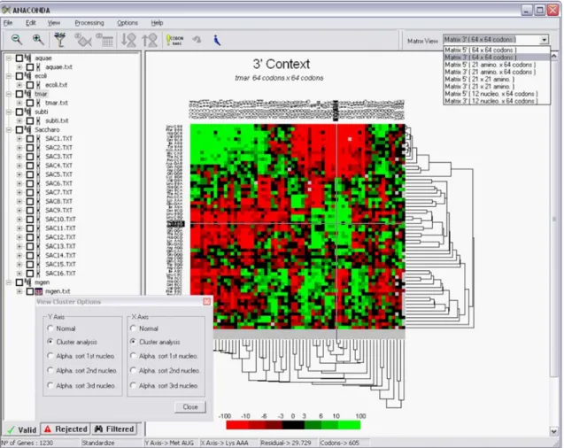
Figure 1. Main window of the software package ANACONDA for two-codon context analysis at the ORFeome map level. The left panel presents a hierarchical tree
of all genomes under analysis by ANACONDA. The Tab Valid includes all individual ORFs used to determine context bias and to build the respective map, while the Tab Reject allows visual inspection of ORFs that do not comply with the criteria selected during the opening of the ORFeome. An ORFeomic map for two-codon context bias obtained with the total set of predicted coding sequences of Thermotoga maritima (accession number AE000512 from GenBank), is shown.
Figure. 2. Main window of the software package ANACONDA for two-codon context analysis in total genomes at the gene view level. Individual ORFs that were
used to calculate codon context bias are shown in the hierarchical left panel. Clicking on one of them changes the main panel into the gene view layout. This is composed of a header with the name of the ORF as stated in the original file and the sequence itself. This sequence is coloured according to the residual colour scale obtained for that ORFeome, i.e. each codon pair is coloured in the ORF sequence with the same colour scale that it had in the ORFeome map for two-codon contexts. Rare codons are highlighted using circles.
Figure 3. Main window of the software package ANACONDA for two-codon
context analysis at the ORFeome comparison level. When more than 3 ORFeomes
are processed by ANACONDA it is possible to build a large-scale comparative map, as shown in the main right panel of the software’s window. In this map, each column represents one ORFeome, with one line for all possible combinations of two consecutive codons. Visual comparison of different ORFeomes is possible because all ORFeomes are normalized to a given size and aligned using the same context order.