Diagnosis of Switching Systems using Hybrid Bond Graph
Taher Mekki1, Slim Triki1 and Anas Kamoun1 1
Research Unit on Renewable Energies and Electric Vehicles (RELEV), University of Sfax Sfax Engineering School (ENIS), Tunisia
Abstract
Hybrid Bond Graph (HBG) is a Bond Graph-based modelling approach which provides an effective tool not only for dynamic modeling but also for fault detection and isolation (FDI) of switching systems. Bond graph (BG) has been proven useful for FDI for continuous systems. In addition, BG provides the causal relations between system’s variables which allow FDI algorithms to be developed systematically from the graph. There are many methods that exploit structural relations and functional redundancy in the system model to find efficient solutions for the residual generation and residual evaluation steps in FDI of switching systems. This paper describes two different techniques, quantitative and qualitative, based on common modelling approach that employs HBG. In quantitative approach, global analytical redundancy relationships (GARRs) are derived from the HBG model with a specified causality assignment procedure. GARRs describe the system behaviour at all of its operating modes. In qualitative approach, functional redundancy can be captured by a Temporal Causal Graph (TCG), a directed graph that may include temporal information.
Keywords: Hybrid Bond Graph, Global Analytical Redundancy Relation, Temporal Causal Graph.
1. Introduction
Several physical systems with switching are nonlinear dynamic systems. When switching occurs, the system may change its mode of operation. If a system has n switching states, then it gives rise to 2n possible operating modes. One way to represent mode switching is to generate 2n sets of differential-algebraic equations (DAEs). Each set describes continuous behaviour of system in that particular mode. In practice, not all modes are practically realizable. Many recent researches on switching systems have been devoted to the synthesis of control laws that guarantee not only the stability but also good performances [1]. The control algorithms are generally developed considering that the system works in normal situation. Unfortunately, when failures occur, these algorithms become inefficient and even dangerous for the system itself or its environment. In order to reach higher performances and more rigorous security specifications, a Failure Detection and Isolation system has to be implemented. The literature in that field is abundant and different solutions have been proposed for continuous or discrete, linear and non linear
systems. However, only few solutions have been proposed for switching systems.
Traditionally, two different communities: (1) the Systems Dynamics and Control Engineering (FDI) community (e.g., [2,3]), and (2) the Artificial Intelligence Diagnosis (DX) community (e.g., [4,5]), have developed model-based diagnosis approaches. The two communities have employed different kinds of models, and made different assumptions concerning robustness of the generated solution with regard to modeling errors, measurement noise, and disturbances. The general principle of all model-based FDI approaches is to compare the expected behavior of the system, given by model, with its actual behavior. The first step of a FDI procedure consists in generating a set of residuals. These residuals are special signals that reflect the discrepancy between the two behaviors. Analytic Redundancy Relation (ARR) methods are classically used for residual generation in the FDI community [6]. The DX community has developed methods such as possible conflicts [7,8], and analysis of temporal causal graphs [9,10] for diagnosis of continuous systems. These methods are based on the structural analysis of dynamic models, much like the ARR schemes developed by the FDI community. The two communities use different algorithms, but the overall framework for fault isolation is similar, defined by a two-step process: (i) residual generation, followed by (ii) residual evaluation [2,3].
2. Quantitative hybrid bond graph-based
fault detection and isolation
2.1 Analytical Redundancy Relations (ARRs) and
Global ARRs
An ARR obtained from a physical law represents some conservation phenomena: Bernoulli equation etc. in hydraulic domain; Newton’s law etc. in mechanical domain; and Kirchoff’s law etc. in electrical domain. The ARRs for ordinary (non hybrid) system can be derived algorithmically from derivative causality bond graph model or Diagnostic Bond Graph (DBG) [17,18]. Whereas the bond graph model for hybrid system with discrete mode changes is called the Hybrid Bond Graph, and the GARRs are derived in similar manner from differentially causalled HBG or Diagnostic Hybrid Bond Graph (DHBG). A DHBG is a HBG which describes the behavior of a hybrid system at all modes based on unified set of causality assignment [19]. In other words, for a given DHBG, a reassignment of causality to the HBG is not required to describe the behavior of the system at different operating modes. This unique feature of DHBG implies that the causal paths of graph maintain the same structure, except that some of the sub-paths are eliminated due to the OFF states of the controlled junctions. Based on these uniform causal paths, a set of unified relations is derived to describe the hybrid system at all modes. This set of relations which is called Global ARRs (GARRs), are utilized as ARRs for the hybrid systems. Likewise for continuous system, the GARRs provide a convenient tool to deduce the fault detectability and isolability of a hybrid system. To illustrate how to derive the GARR for FDI application, consider the three coupled tanks depicted in Fig. 1. These tanks are connected by pipes which can be controlled by different valves. Water can be filled into the left and right tanks using two identical pumps. Measurements available from the process are the continuous water levels hi(t) of each tank. The connection
pipe, with valve R12 (res. R23), between the tank 1 and 2
(res. 2 and 3) is placed at a height of 0.5m (res. 0.7m).
R1 R2
R12
C1 C2
P Qp1 h1 h2
C3
R23
h3 Qp2 P
0.5 0.7
Pc1 Pc2 Pc3
12
R
f R23
f
1
R
f fR2
Fig. 1 Three Tank System.
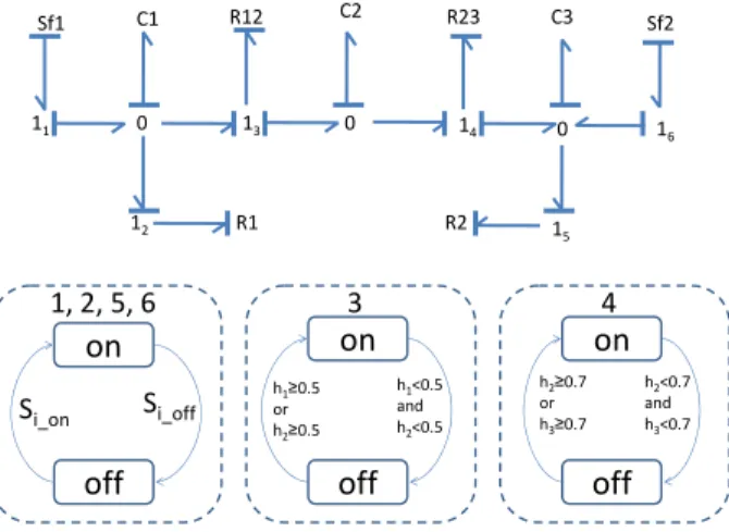
Fig. 2 shows the hybrid bond graph model of this system. The two flow sources into tanks 1 and 3 are indicated by Sf1 and Sf2, respectively. The tank capacities are shown as
C1, C2 and C3. The pipes are modeled by resistances R1,
R12, R23 and R2. Pumps and valves are modeled by
controlled junctions, which are shown in the figure as junctions with subscripts (11, 12, 15, and 16). The control
signals for turning these junctions on and off are generated by the finite state automata in Fig. 2. For autonomous transitions in the system, also modeled by controlled junctions, the transition conditions computed from system variables (junctions 13 and 14). A mode in the system is
defined by the state of the six controlled junctions in the hybrid bond graph model. Therefore, theoretically the system can be in 6
2 different modes.
Sf1
0
R1 C1
0 C2
0
R2
C3 Sf2
11 13 14 16
12 15
R12 R23
on
off
1, 2, 5, 6
Si_on Si_off
on
off
3
h1≥0.5 or h2≥0.5
on
off
4
h1<0.5 and h2<0.5
h2≥0.7 or h3≥0.7
h2<0.7 and h3<0.7
Fig. 2 HBG of the three tank system.
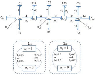
Fig. 3 shows the DHBG model of the hybrid tank system deduced from the three step procedure Hybrid Procedure Assignment Causality Sequential (SCAPH) and Model Approximation (MA) detailed in [19]. First step, a Rs
component is added to every sensor junction; in this example a very-high resistive component is added to the junction 01, 02 and 03. The second step is to apply the
SCAPH algorithm. In this step, all controlled junction are assigned with their preferred causality. As shown in Fig. 3, the output variables of the controlled-junctions 1c1 and
1c2 (e5 and e10, respectively) are assigned as inputs of the
1-port component (
12 R and
23
R , respectively). There is no source connected to the controlled-junction. Then the two sources Qp1 and Qp2 are assigned with their preferred
causality. Since the DHBG is required to generate the GARR, the three storage components C1, C2 and C3 are
indifferent causality. In our case Rs added to the junction
01 and 03 are redundant and, therefore, are removed from
the DHBG model of Fig. 3.
Qp1 01
R1 C1
02
C2
03
R2 C3
Qp2
1c1 1c2
R12 R23
De1 De2 De3
1 2
3 4
5
6 7
8
10
11 12
13 14
1
α α1 α2 α2
2
α
1
α
9
Rs
1c1
h1≥0.5 or h2≥0.5
1c2
h1<0.5 and h2<0.5
h2≥0.7 or h3≥0.7
h2<0.7 and h3<0.7
1 1
α =
1 0
α =
2 1
α =
2 0
α =
Fig. 3 DHBG of the three tank system.
The constitutive relation of the Rs component connected to
the junction 02 is f8=0 . From the DHBG, the constitutive
relations of junctions 01, 1c1, 02, 1c2 and 03 are given by the
following equations: Junction 01
1 2 3 1 4 0
f −f −f −α f =
(1)
Junction 1c1
4 5 6 0
e − −e e =
(2)
Junction 02
1f6 f7 f8 2f9 0
α − − −α = (3)
Junction 1c2
9 10 11 0
e −e −e = (4) Junction 03
2 11f f14 f12 f13 0
α + − − = (5)
Where
1 2
1 1 2
12
4 6
2 1 2
12
1 2 1 2 1 2
12
4 6 1 2 1
0 if 0.5 and 0.5
1
( 0.5) if 0.5 and 0.5
1
( 0.5) if 0.5 and 0.5
1
( )* if 0.5 and 0.5
(max( ,0.5) max( ,0.5))*(max( ,0.5)
h h
De h h
R
f f
De h h
R
sign De De De De h h
R
f f sign De De De
< <
⎧ ⎪
⎪ − > <
⎪ ⎪
= =⎨−⎪ − < >
⎪
⎪ − − > >
⎪ ⎩
⇒ = = − −max(De2,0.5))
2 3
2 2 3
23 9 11
3 2 3
23
2 3 2 3 2 3
23
9 11 2 3 2
0 if 0.7 and 0.7
1
( 0.7) if 0.7 and 0.7
1
( 0.7) if 0.7 and 0.7
1
( )* if 0.7 and 0.7
(max( ,0.7) max( ,0.7))*(max( ,0.7) ma
h h
De h h
R f f
De h h
R
sign De De De De h h R
f f sign De De De
< < ⎧
⎪
⎪ − > <
⎪ ⎪ = = ⎨−
− < >
⎪ ⎪ ⎪
− − > >
⎪ ⎩
⇒ = = − − x(De3,0.7))
Three structurally independent GARRs can be generated from (1), (3) and (5) after eliminating the unknown variables and obtained as follows:
1 1 1 1
1 1
1 2 1 2
12
1 1
(max( , 0.5) max( , 0.5)) * (max( , 0.5) max( , 0.5))
p
d
GARR Q C De De
dt R
sign De De De De
R
α
= − −
− − −
(6)
1
1 2 1 2
12 2
2 2 2 3 2 3
23
2 (max( ,0.5) max( ,0.5))*(max( ,0.5) max( ,0.5))
(max( ,0.7) max( ,0.7))*(max( ,0.7) max( ,0.7))
GARR sign De De De De
R
d
C De sign De De De De
dt R
α
α
= − −
− − − −
(7)
2
2 3 2 3
23
2 3 3 3 2
3 (max( ,0.7) max( ,0.7))*(max( ,0.7) max( ,0.7))
1 p
GARR sign De De De De
R d
Q C De De
dt R
α
= − −
+ − −
(8)
2.2 Fault detectability and fault isolability
Unlike continuous systems, hybrid systems are multiple modes in nature. This feature suggests that the system’s fault detectability and fault isolability are required to be evaluated at different operating modes for effective FDI analysis and designs. The unified characteristic of the GARRs provide a convenient way to generate the Fault Signature Matrix (FSM) of each operating mode. Table 1 shows the FSM of the three tank system and table 2 describes the modes. The fault detectability and fault isolability of each parameter is gained from the {Db, Ib}
values of the four FSMs. This information can be summarized in table 3.
Table 1: FSM for the three tank system
GARR1 GARR2 GARR3 Db Ib
R1 1 0 0 1 0
C1 1 0 0 1 0
R12 α1 α1 0 α1 α1
C2 0 1 0 1 1
R23 0 α2 α 2 α2 α2
C3 0 0 1 1 0
Table 2: Modes of the system Modes
α
1α
2Mode 1 1 1 Mode 2 1 0
Mode 3 0 1
Mode 4 0 0
Table 3: Fault Detectability and fault Isolability of components
θ Detectability Isolability
R1 all-mode Nil
C1 all-mode Nil
R12 Mode 1, 2 mode 1, 2
C2 all-mode all-mode
R23 Mode 1, 3 mode 1, 3
C3 all-mode Nil
R2 all-mode Nil
In this work, MATLAB 7.0 is used to simulate the model of the tank system. The parameters of the system are fixed as follow; R1= R12= R23= R2=1m-1s-1, C1= C2= C3=1kg -1m4s2, and simulation time is fixed to 10s with sampling
time ts=0.01s. The inputs Qp1(t), Qp2(t) are presented in
Fig. 4.
0 1 2 3 4 5 6 7 8 9 10
0 0.5 1
t(s)
Q
p1(
k
g/
s
)
0 1 2 3 4 5 6 7 8 9 10
0 0.5 1
t(s)
Q
p2(
k
g
/s
)
Fig. 4 Inputs on the system.
A fault is simulated in R12 component where its parametric
value changes abruptly from 1 to 5 at t=1s. The fault profile is shown in Fig. 5. Figure 6 depicts the measured variables and the switches signals.
0 1 2 3 4 5 6 7 8 9 10
1 2 3 4 5
t(s)
R
1
2(
m
-1s
-1
)
Fig. 5 Fault profile in R12 component.
0 1 2 3 4 5 6 7 8 9 10
0 0.25 0.5 0.75 1
t(s)
h1(
m
)
0 1 2 3 4 5 6 7 8 9 10
0 0.1 0.2 0.3 0.4 0.5 0.6 0.7 0.8
t(s)
h2(
m
)
1.7
0 1 2 3 4 5 6 7 8 9 10
0 0.2 0.4 0.6 0.8
t(s)
h3
(m
)
0 1 2 3 4 5 6 7 8 9 10
0 0.5 1
t(s)
al
ph
a1
0 1 2 3 4 5 6 7 8 9 10
-0.5 0 0.5
t(s)
al
ph
a2
Fig. 6 Plot of measured variables and operating modes alpha 1 and 2.
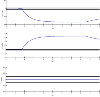
The residuals GARR1, GARR2 and GARR3 due to the fault in R12 are shown in Fig. 7 where line denotes the
thresholds reε1= ±0.02,ε2= ±0.01andε3= ±0.01.
0 1 2 3 4 5 6 7 8 9 10
-0.4 -0.2 0 0.2
t(s)
GA
R
R
1
0 1 2 3 4 5 6 7 8 9 10
-0.2 -0.1 0 0.1 0.2 0.3 0.4
t(s)
G
A
RR2
0 1 2 3 4 5 6 7 8 9 10
-0.04 -0.02 0 0.02 0.04
t(s)
GA
R
R
3
Fig. 7 Residuals responses for single fault in R12 component.
initiate at Mode 4, i.e.α1=0,α2=0 , which is a non-observable mode. Hence the fault can not be detected until the system enters a mode in which fault is detectable, i.e. at time t=1.7s (see Fig. 6) when the system change to the Mode 2 (α1=1,α2=0). Fig. 7 reveals that GARR1 and GARR2 are sensitive to fault. From the FSM table at that mode, R12 has fault signature [1 1 0]. According to the
FSM table 3, R12 is not detectable at Mode 3.
3. Qualitative hybrid bond graph-based
detection and isolation
3.1 Temporal Causal Graph and Parametrized
Causality
The DX community from the field of Artificial Intelligence, have developed a number of diagnosis algorithms based on consistency-based techniques [5]. There are many works in the literature that use the BG and HBG modeling language for this purpose. For example, [9] developed a diagnosis schema, which called TRANSCEND, based on the qualitative analysis of fault transient information for diagnosis of continuous systems. Since hybrid systems cannot be described by a single continuous or discrete event model, [20] extend the TRANSCEND system to Hybrid TRNASCEND where the diagnosis algorithms use a combination of qualitative and quantitative reasoning mechanisms. Authors in [21] propose a qualitative event-based approach to fault diagnosis of hybrid systems that extends the TRANSCEND and Hybrid TRANSCEND methodologies to incorporating discrete faults.
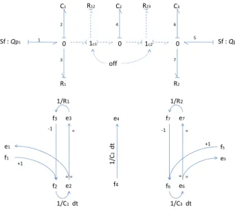
In all proposed frameworks, system uses a Temporal Causal Graph (TCG) model in order to analysis fault transients. Then, the diagnosis is based on this analysis, where observed deviations from nominal behavior expressed in qualitative form are compared against qualitative predictions of faulty behavior, i.e., fault signature, to isolate faults. For a particular mode, the TCG is constructed based on the system equations for that mode. Using the bond graph model this process is made easy. First, causality is assigned using SCAP [22], or, in the case of HBGs, may be reassigned based on the assignment of the previous mode using Hybrid SCAP [22,23,24]. After that, the bonds are converted to system variables and the bond graph elements are converted into labeled edges connecting the variables of their associated bonds (see Fig. 8). Signal links are converted into single edges, with the qualitative label corresponding to the qualitative relationship between the variables.
Fig. 8 Temporal Causal Graph transformations.
Fig. 9 shows a bond graph of the three-tank system and its corresponding TCG in the case when control junctions are both in mode OFF.
0
1 2
3
Sf : Qp1
C1
R1
4
C2
0 0
5 6
7
Sf : Qp2
C3
R2
1c1 1c2
off
R12 R23
f1
e1
f3 e3
f2 e2
e5
f5
f7 e7
f6 e6 ‐1
‐1
+1
+1 =
= =
=
f4
e4
1/C1dt 1/C3dt
1/R1 1/R2
1/
C
2
dt
= =
Fig. 9 Temporal Causal Graph of Three Tank System in mode 00.
The numbered bonds are converted to corresponding variables with subscript indicating the bond number. For example, bond 3 becomes e3and
f
3. The resistor relates these two variables, i.e.,3 3
1
1
f e
R
= . The causality of the
the given causality. For the capacitance, the relationship between
f
2and e2is an integration, hence the dt label. Junctions sum one type of variable according to the bond signs, and set the other type equal. For the 0-junction, bond 2 is determining the effort of the junction, so e1and3
e
are set equal to e2 . According to the bond signs, f2= −f1 f3. Sincef
2must be determined,1 f and
3
f
causally affectf
2with labels +1 and -1, respectively. In order to deal with the change of causality, the TCG can be derived for each possible system configuration or mode. However, in case of many locally acting switches, the combinatorial explosion quickly leads to an intractable problem. These problems can be mitigated to some extent by dynamically generating the TCG of each possible system mode in response to a failure. This may still result in a problem with large computational complexity which can be further reduced by measuring system variables that indicate specifically which local switches may have occurred and predictions for each of the variables that determine different causal assignments are required to be made and analyzed [25]. Once a set of possible TCGs is available, Gaussian decision techniques have been applied to compute the most likely mode of continuous behavior [9]. Others attention to hybrid diagnosis [26] concentrates on efficiently processing a set of TCGs. [27] describes how a hybrid model can be made amenable to the diagnosis algorithms that were developed in [28] by systematically generating one parametrized TCG. In this graph, the directed links are enabled by conditionals that correspond to the mode in which these links are present. The result is a set of predictions that are parametrized by the state of the local switches and the diagnosis problem then becomes one of constraint satisfaction [16]. The solution to this constraint satisfaction problem contains the possible parameter changes (i.e., the faults) and the effect on the system mode that this is required to have.3.2 Parametrized Causality: Temporal Causal Matrix
To derive qualitative predictions, the system may be written as a directed graph that captures the causal (directed) relations between system variables [27]. Hence, the TCG can be represented by a weighted adjacency matrix where the columns are cause and rows are the effect variables and the entries capture the parameters on the graph edges. This is called the Temporal Causal Matrix (TCM). In the case of switched systems, modeled discontinuities result in causal changes. Therefore, the TCM may take several different forms and so do the corresponding predictions of future behavior, depending on whether a mode change occurs. To handle the change in TCM, the causal relations can be parametrized to make
them dependent on the mode of operation. To this end, first the system is described in a noncausal form by using implicit equations. An implicit model of the three-tank (see Fig. 1) consists of the following equations:
1 1 12 2 1 12
2 2 23 3 2 23
1 1 1 12
2 12 23
3 23 2 2
1
1 1 1
1 1 1
12 12 12
1
2 2 2
1
3 3 3
2 2 2
23 23
( ) (1 ) 0
( ) (1 ) 0
0 0
0
0 0
0
0 0 0
c R c R
c R c R
c p R R
c R R
c R R p
c c
R R
R R
c c
c c
R R
R R
P P P f
P P P f
f Q f f
f f f
f f f Q
P C f
P R f
P R f
P C f
P C f
P R f
p R f
α α
α α
λ
λ λ −
−
−
− + + + − =
− + + + − =
− + + =
− + =
− + − + =
− =
− =
− =
− =
− =
− =
− 23 0
⎧ ⎪ ⎪ ⎪ ⎪ ⎪ ⎪ ⎪ ⎪⎪ ⎨ ⎪ ⎪ ⎪ ⎪ ⎪ ⎪ ⎪ ⎪
⎪ =
⎩
(9)
where λ represents the time differentiation operator and λ-1 indicates integration over time. From Eq. (9.1), i.e.
(
) (
)
1 Pc1 PR12 PC2 1 1 fR12 0
α
− + + + −α
= , in case the water in tank 1 or tank 2 reach the level 0.5 the pipe12
R become conducting, α1 = 1, and Pc1−Pc2 =PR12, else, α1=0, and
12 0 R
f = . The TCM for this system of equations contains the relations between each of the variables. For example, Eq. (9.6) embodies a temporal relation between
1 c
P and
f
c1and Eq. (9.2) a relation betweenP
c2,P
c3and23 R
P that is only active when α2= 1.
and resistors define instantaneous magnitude relations, and capacitors and inertias define temporal effects on causal edges. For this example, to simplify the TCG structure, all
=
links and corresponding variables have been removed.fR1
Qp1 fc1 p
c1 pR1 pc2 pR12 fR12 pR2 2 1R 1 1R 1 1 1 C−λ−
12 1R -1 1 -1 1
α −α1
1
fc2
1
1 1
2 C −λ−
fR23
pR23 pc3
2 α −α2
23
1R
fc3
fR2
1 -1
1 1
3 C−λ−
Qp2
1 1
Fig. 10 Temporal Causal Graph of Three Tank System.
The resulting TCM is given by: 1
1 1
1
2 2
1
1 0 0 1 0 1 0 0 0 0 0 0 0 0
1 0 0 0 0 0 0 0 0 0 0 0 0
0 1 1 0 0 0 0 0 0 0 0 0 0 0
0 0 1 1 0 0 0 0 0 0 0 0 0 0
0 0 0 1 1 0 0 0 0 0 0 0
0 0 0 0 1 1 0 0 0 0 0 0 0 0
0 0 0 0 0 1 1 0 0 1 0 0 0 0
0 0 0 0 0 0 1 0 0 0 0 0 0
0 0 0 0 0 0 0 1 1 0 0 0
0 0 0 0 0 0 0 0 1 1 0 0 0 0
0 0 0 0 0 0 0 0 0 1 1 0 0 1
0 0 0 0 0 0 0 0 0 0 1 0 0
0 0 0 0 0 0 0 0 0 0 0 1 1 0
0 0 λ α α λ α α λ − − − − − − − − − 1 1 1 1 12 12 2 2 23 23 3 3 2 2
0 0 0 0 0 0 0 0 0 0 1 1
c c R R R R c c R R c c R R f P P f P f f P P f f P P f ⎡ ⎤ ⎡ ⎤ ⎢ ⎥ ⎢ ⎥ ⎢ ⎥ ⎢ ⎥ ⎢ ⎥ ⎢ ⎥ ⎢ ⎥ ⎢ ⎥ ⎢ ⎥ ⎢ ⎥ ⎢ ⎥ ⎢ ⎥ ⎢ ⎥ ⎢ ⎥ ⎢ ⎥ ⎢ ⎥ ⎢ ⎥ ⎢ ⎥ ⎢ ⎥ ⎢ ⎥ ⎢ ⎥ ⎢ ⎥ ⎢ ⎥ ⎢ ⎥ ⎢ ⎥ ⎢ ⎥ ⎢ ⎥ ⎢ ⎥ ⎢ ⎥ ⎢ ⎥ ⎢ ⎥ ⎢ ⎥ ⎢ ⎥ ⎢ ⎥ ⎢ ⎥ ⎢ ⎥ ⎢ ⎥ ⎢ ⎥ ⎢ ⎥ ⎢ ⎥ ⎣ ⎦ ⎣ ⎦ (10)
The predictions of the TCM are parametrized by the active mode. This leads to more efficient diagnosis compared to the use of a bank of TCMs, which, in this case of two switches, would consist of four TCMs that need to be processed separately. The fault detectability and fault isolability of each parameter is gained from the {Db, Ib}
values of the four FSMs. This information can be summarized in tables 4, 5, 6, 7 and 8.
Table 4: FSM at mode 1 (α α1= 2=1)
Mode 1 Pc1 Pc2 Pc3 Db Ib
1
R+ 0+ 00 00 1 1
1
C− +- 0+ 00 1 1
12
R+ 0+ 0- 00 1 1
2
C− 0+ +- 0+ 1 1
23
R+ 00 0+ 0- 1 1
3
C− 00 0+ +- 1 1
2
R+ 00 00 0+ 1 1
Table 5: FSM at mode 2 (
α
1=0,α
2 =1)Mode 2
1
c
P Pc2 Pc3 Db Ib
1
R+ 0+ 00 00 1 1
1
C− +- 0+ 00 1 1
12
R+ 0+ 0- 00 1 1
2
C− 0+ +- 00 1 1
23
R+ 00 00 00 0 0
3
C− 00 00 +- 1 1
2
R+ 00 00 0+ 1 1
Table 6: FSM at mode 3 (α1=0,α2=1)
Mode 3 Pc1 Pc2 Pc3 Db Ib
1
R+ 0+ 00 00 1 1
1
C− +- 00 00 1 1
12
R+ 00 00 00 0 0
2
C− 00 +- 0+ 1 1
23
R+ 00 0+ 0- 1 1
3
C− 00 0+ +- 1 1
2
R+ 00 00 0+ 1 1
Table 7: FSM at mode 4 (α α1= 2=1)
Mode 4 Pc1 Pc2 Pc3 Db Ib
1
R+ 0+ 00 00 1 1
1
C− +- 00 00 1 1
12
R+ 00 00 00 0 0
2
C− 00 +0 00 1 1
23
R+ 00 00 00 0 0
3
C− 00 00 +- 1 1
2
R+ 00 00 0+ 1 1
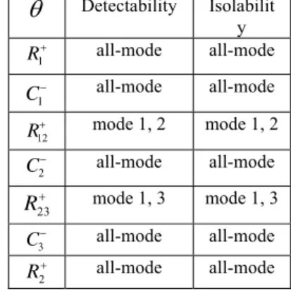
Table 8: Fault Detectability and fault Isolability of components
θ
Detectability Isolability
1
R+ all-mode all-mode
1
C− all-mode all-mode
12
R+ mode 1, 2 mode 1, 2
2
C− all-mode all-mode
23
R+ mode 1, 3 mode 1, 3
3
C− all-mode all-mode
2
R+ all-mode all-mode
4. Conclusions and discussion
issues are not considered in such diagnosis and only abrupt faults are handled. The application of this method is constrained to only open-loop systems because it relies on temporal trends of systems evolution obtained from the measurements which may not show any deviation if they are controlled. It is well known that controllers try to hide the fault effects. The qualitative approach overcomes limitations of quantitative schemes, such as convergence and accuracy problems in dealing with complex non-linearities and lack of precision of parameter values in system models. The qualitative reasoning scheme is fast, but it has limited discriminatory ability.
As presented in this article, a single approach for diagnosis has limitations, and it does not satisfy all the requirements to perform a good diagnosis. Hence, several works can be found in literatures that combine diagnostic approaches. The objective is to find two or several approaches that complete each other, in a way that the qualities of one approach can overcome the drawback of another. In a future work, we will focus on complex models with implicit relations, complex non-linearities, and algebraic loops.
References
[1] D. De Scuter, “Optimal control of a class of linear hybrid systems with saturation”, SIAM Journal of Control Optimization, Vol. 39, No. 3, 2000, pp. 834-851.
[2] J. J. Gertler, “Fault detection and diagnosis in Engineering Systems”, Ph.D. Dissertation, George Mason University, Fairfax, Virginia, 1998.
[3] R. J. Patton, P. M. Frank and R. N. Clark, Issues in fault diagnosis for dynamic systems, Springer Verlag, New York, 2000.
[4] w. C. Hamascher, J. Decleeer and L. Console, “reading in model based diagnosis”, Morgan-kaufmann Pub, San mateo, 1992.
[5] R. Reiter, “A theory of diagnosis from first principles”, Artificial Intelligence, 1987, Vol. 32, pp. 57-95.
[6] M. Staroswiecki and G. Comtet-Verga, “Analytical redundancy relations for fault detection and isolation in algebraic dynamic systems, Automatica, 2001, pp. 687-699 [7] B. Pulido and C. Alonso-Gonzlez, “An alternative approach
to dependency-recording engines in consistency-based diagnosis”, Atificial Intelligence, 2000, pp. 111-120.
[8] B. Pulido and C. Alonso-Gonzlez, “A compilation technique for consistency-based diagnosis”, IEEE Trans, 2004, pp. 2192-2206.
[9] P. J. Mosterman and G. Biswas, “Diagnosis of continuous valued systems in transient operating regions, IEEE Trans, 1999, pp. 554-565.
[10] E. J. Manders, S. Narasimhan, G. Biswas and P. J. Mosterman, “A combined qualitative/quantitative approach for fault isolation in continuous dynamic systems, IFAC, 2000, pp. 1074-1079.
[11] W. Borutzky, “”Representing discontinuities by means of sinks of fixed causality”, International Conference On Bond Graph Modeling, 1995, Vol. 27, pp. 65-72.
[12] P. J. Gawthrop, “Hybrid bond graph using switch I and C components”, International Conference On Bond Graph modeling, 1997.
[13] J. E. Stromberg, J. Top and U. Sodermann, “Variable causality in bond graphs by discrete effects, International Conference On Bond Graph modeling, 1993, pp. 115-119. [14] C. B. Low, D. W. Wang, S. Arogeti and Z. J. Bing,
“Causality assignment and model approximation for quantitative hybrid bond graph-based fault diagnosis, IFAC, 2008, pp. 10522-10527.
[15] J. Feenstra, P. J. Mosterman, G. Biswas and R. J. Breedveld, “Bond graph modeling procedures for fault detection and isolation of a complex flow processes, International Conference On Bond Graph modeling, 2001, Vol. 33, pp. 77-82.
[16] M. Torrens, R. weigel and B. Faltings, “Java Constraint library”, Workshop on Constraints and Agents, 1997. [17] A. K. Samantary, S. K. Ghoshal, S. Chakraborty and A.
Mukherjee, “Improvements to single fault isolation using estimated parameters”, Simulation: Transactions of the Society for Modeling and simulation International, 2005, Vol. 81, No. 12, pp. 827-845.
[18] A. K. Samantary, K. Medjaher, B. O. Bouamama, M. Staroswiecki and G. Dauphin-Tanguy, “Diagnostic bonf graphs for online fault detection and isolation”, Simulation Modeling Practice and Theory, 2006, Vol. 14, No. 3, pp. 237-262.
[19] C. B. Low, D. Wang, S. Arogeti and J. B. Zhang, “Causality Assignment and Model approximarion for Hybrid Bond Graph”, IEEE Transactions on Automation Science and Engineering, Vol. 7, No. 3, 2010, pp. 570-580.
[20] S. Narasimhan, “Model-based diagnosis of hybrid systems”, Ph. D. Dissertation, Vanderbilt University, 2002.
[21] M. J. Daigle, “A qualitative event-based approach to fault diagnosis of hybrid systems, Ph. D. Dissertation, Vanderbilt University, 2008.
[22] I. Roychoudhury, M. Daigle, G. Biswas, X. Koutskous and P. J. Mosterman, “A method for efficient simulation of hybrid bond graphs, International Conference On Bond Graph modeling, 2007, pp. 177-184.
[23] D. C. Karnopp, D. L. Margolis and R. C. Rosenberg, “Modeling and simulation of Mechatronic Systems, New York: John Wiley & Sons, 2000.
[24] M. Daigle, I. Roychoudhury, G. Biswas and X. Koutskous, “Efficient simulation of component-based hybrid modeld represented as hybrid bond graphs, Institute for Software Integrated Systems, Vanderbilt University, 2006.
[25] S. Narasimhan, G. Biswas, G. Karsai, T. Pasternak and F. Zhao, “Building observers to address fault isolation and control problems in hybrid dynamic systems, In proceeding of the IEEE International Conference on Systems, 2000, pp. 2393-2398.
[26] S. Mclraith, G. Biswas, D. Clancy and V. Gupta, “Hybrid systems diagnosis”, Springer Verlag, 2000.
[27] P. J. Mosterman, “Diagnosis of physical systems with hybrid models using parametrized causality, Institute of robotics and mechatronics , Germany, 2001.