SRef-ID: 1432-0576/ag/2005-23-1455 © European Geosciences Union 2005
Annales
Geophysicae
Excitation of Alfv´en impulse by the anomalous resistance onset on
the auroral field lines
V. Pilipenko1, N. Mazur1, E. Fedorov1, T. Uozumi2, and K. Yumoto2 1Institute of the Physics of the Earth, Moscow, Russia
2Space Environment Research Center, Kyushu University, Fukuoka, Japan
Received: 11 September 2004 – Revised: 8 March 2005 – Accepted: 29 March 2005 – Published: 3 June 2005
Abstract. The onset of anomalous resistance in a layer on auroral field lines is shown to be accompanied by the excita-tion of an Alfv´enic impulse (AI). The generated AI marks the transition of the global magnetosphere-ionosphere instability into an explosive phase with positive feedback. The spatial structure of this impulse both in space and on the ground has been described analytically and numerically under the thin layer approximation. The field-aligned currents transported by the Alfv´enic impulse are concentrated near the edges of the layer with anomalous resistivity, whereas the reverse cur-rents are spread throughout the layer. For some parameters of the layer the ionospheric attenuation of even small-scale structures is not dramatically large, so the magnetic response to the generated AI may be observed on the ground. The considered event on 3 January 1997 with magnetic-auroral intensification observed by ground magnetometers and Polar UV imager agrees with the model proposed.
Keywords. Magnetospheric physics (MHD waves and in-stabilities; magnetosphere-ionosphere interactions; auroral phenomena)
1 Introduction
Though Pi2 pulsations belong to the most well-known types of ULF waves, still there is no confirmative physical interpre-tation of their generation mechanism. To some extent, this situation is quite natural because it is unrealistic to develop a final theory of Pi2 before the build-up of a general theory of substorms. Nowadays, the substorm theory is still an un-resolved problem of geophysics. However, as seismic waves provide information about earthquakes, though the physics of earthquakes is not fully understood, in a similar way the Pi2 waves may be used as a tool for the understanding and monitoring of the substorm process.
Correspondence to:V. Pilipenko ([email protected])
A typical Pi2 waveform-damping short train implies that Pi2 is a transient response to some rapid large-scale change of the night-side magnetospheric current system (Baumjo-hann and Glassmeier, 1984; Olson, 1999). Because of multi-ple rapid plasma processes in the nightside magnetosphere, it should be expected that Pi2-like transient disturbances can be triggered by several possible magnetospheric drivers. Gen-eral association within a few minutes was established be-tween the Pi2 waves and the substorm onset, auroral breakup, onset of geomagnetic bay, and explosive phenomena in the nightside magnetosphere, such as the cross-tail current dis-ruption, dipolarization, X-line formation, bursty bulk flows, etc. (Shiokawa et al., 1998; Kepko and Kivelson, 1999; Liou et al., 1999, 2000; Kepko et al., 2001). Moreover, the exis-tence of several onset mechanisms or their synthetic com-binations is possible (Lui, 1996). The growth phase of a substorm is often accompanied by a series of localized au-roral activations, from small-scale arc activation to pseudo-breakup (Shiokawa et al., 2002). Probably only one from this series of activations is the “main onset”, leading to the explo-sive substorm development. Moreover, transient magnetic signals can be excited in the ionosphere by sudden changes in the ionospheric conductance under the impact of precipi-tating electrons (Maltsev et al., 1974), or by the switch-on of the energetic particles source (Trakhtengertz and Feldstein, 1988). Thus, to identify a specific mechanism of the sub-storm global instability, more detailed timing and examina-tion of the onset fine structure are necessary.
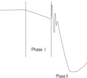
Phase I
Phase II
Fig. 1.A schematic scenario of the temporal two-stage evolution of the substorm explosive phase.
2 General physics of the magnetosphere-ionosphere in-teraction
First, we outline the role of anomalous resistance in the magnetosphere-ionosphere interaction. The origin of a sub-storm is related to the reconfiguration of global currents in the nightside magnetosphere. The key element of this recon-figuration is the disruption of the cross-tail current and its divergence into field-aligned currents towards or away from the ionosphere. This process may be visualized as a sradic electric discharge of the magnetospheric cross-tail po-tential through the ionosphere, though the specific mecha-nism of this global instability has not been firmly identified yet. In the region of upward field-aligned currentj0the emer-gence of an anomalous resistivity layer (ARL) with a finite field-aligned conductivityσkresults in the emergence of an anomalous electric field Ek≃j0/σk. This field-alignedEk accelerates down-going electrons that precipitate in the iono-sphere. The accelerated electrons, in turn, cause additional ionization of the ionosphere and activation of the auroral ac-tivity. The ionospheric ionization and relevant modification of the ionospheric conductance make feasible various mecha-nisms of feedback in the coupled ionosphere-magnetosphere system (Lysak and Dum, 1983; Pokhotelov et al., 2001; Lysak and Song, 2002). In a general sense, it may be specu-lated that the cause of substorm is some global instability of the ionosphere-magnetosphere system. After the turn-on of the positive feedback in the system this instability transforms itself into an explosive phase with a much higher, possibly non-linear, growth rate.
At the same time the sudden “switch-on” of the anoma-lous resistivity results in the excitation of AI. Details of the excitation mechanism and peculiar spatial structure of this impulse will be considered in this paper. According to the proposed scenario, the AI occurrence signifies the switch-on ofσkalong an auroral field line and thus is the indicator of the transition of a global magnetospheric instability into the
ionosphere-coupled phase with a much higher growth rate. The occurrence of resonant features of the ionosphere-magnetosphere system, such as the magnetospheric Alfv´en resonator (with typical eigenfrequencies at auroral latitudes
f∼10 mHz), ionospheric Alfv´en resonator (f∼few Hz) (Belyaev et al., 1990), and the resonator formed between the ionosphere and the auroral acceleration region (f∼few tenths of Hz) (Pilipenko et al., 2002) can produce an oscilla-tory transient response to the excited AI.
Thus, the temporal evolution of a substorm onset can be visualized as a sequence of the following phases, as schemat-ically illustrated in Fig. 1:
I. Growth of the field-aligned current j0 due to energy disbalance in the nightside magnetosphere. At this stage there is still no feedback between the magneto-sphere and ionomagneto-sphere. This stage could be revealed from ground magnetograms as a gradual slow decrease of the H component of the geomagnetic field, and can be coined as a “substorm precursor” (Groot-Hedlin and Rostoker, 1987). At some moment, whenj0exceeds a plasma instability threshold the sudden (on MHD time scale) onset of anomalousσkoccurs. This moment, as suggested by Arykov and Maltsev (1983), is to be ac-companied by the appearance of transient AI.
II. Acceleration of precipitating electrons by anomalous
Ek and modification of the ionospheric conductance, thus establishes a feedback between the ionosphere and the magnetosphere.
From the scenario outlined above it follows that the tran-sition from phase I to phase II actually means a transfer of the global magnetospheric instability into an explosive phase (detonation) with a positive ionospheric feedback.
3 MHD model of a thin ARL
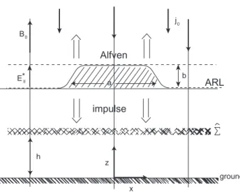
Here we develop a mathematical formalism for the descrip-tion of the AI generadescrip-tion during the switch-on of anomalous resistivity on auroral field lines. We adapt the ARL model, schematically shown in Fig. 2, where the straight geomag-netic field is directed vertically up,B0=B0z. The homoge-ˆ neous magnetospheric plasma has zero transverse static con-ductivity and infinite field-aligned concon-ductivityσk=∞. Only at some altitude, which is considered to be the origin of the field-aligned coordinatez, the finiteσkoccurs inside the ARL with the thicknessband width 2a.
The considered mathematical model is based on the sys-tem of Maxwell’s equations
∇ ×E= −1
c∂tB, ∇ ×B=
4π
c j, (1)
augmented by Ohm’s law
j⊥=6AVA−1∂tE⊥, jz=σkEz, (2)
In this system the possible MHD disturbances are de-scribed by the following decoupled equations for Alfv´en waves, carrying the field-aligned current jz, and
compres-sional waves, carrying the field-aligned magnetic field dis-turbanceBz:
∂t tjz−VA2∂zzjz= c2
4π∇
2
⊥∂t
σk−1jz
,
∂t tBz−VA2∇
2B
z=0. (3)
We assume that the ARL is a thin layer as compared to the Alfv´en wave length. Therefore, the thin layer approximation can be used, that is the ARL thicknessb→0, whereas its total resistanceQ(x, y, t )=b/σkremains finite.
In this approximation the simple Alfv´en wave equation is valid in the upper (z>0) and lower (z<0) hemi-spaces
∂t tjz−VA2∂zzjz=0. (4) This equation must be supplemented with two boundary con-ditions at the interfacez=0 between two hemi-spaces, sepa-rated by a thin layer (b→0) with the resistivityQ. The first condition is the requirement of the continuity of field-aligned current jz(x, y, z, t ) across the ARL, which enables us to
consider the functionjz(0)(x, y, t )=jz(x, y,0, t )(the
super-script (0) indicates that the current is considered inside the ARL). The second boundary condition is obtained by inte-gration of the first equation from the system (3) across the layer and subsequent transition to the limitb→0, as follows {∂zjz}z=0+ ∇⊥2∂t
h
R(x, y, t )jz(0)i=0. (5)
Here R(x, y, t )= c
2
4π VA2Q=6AQV
−1
A is the
normalized resistance of the ARL, and
{∂zjz}z=0=∂zjz(x, y,+0, t )−∂zjz(x, y,−0, t ) is the jump in the current density derivative across the ARL.
4 Generation of Alfv´enic impulse during the switch-on of anomalous conductivity
Let us suppose that att <0 a steady homogeneous current
jz(x, y, z, t )=j0flows along the field lines with zero resis-tanceQ=0. Then, at t≥0 anomalous resistivity is turned on, described by some functionQ(x, y)>0 at the planez=0 (Fig. 2). The onset ofσk induces the disturbance of field-aligned current inside the ARL, which is characterized by the current densityjzA(x, y, t )=jz(0)(x, y, t )−j0. The
solu-tion of Eq. (4) for t≥0 for the whole space is determined by the functionjzA(x, y, t ), defined at the borderz=0. This
solution evidently has the form of outward propagating dis-turbances:
jz(x, y, z, t )=j0+jzA(x, y, t−z/VA), z≥0;
jz(x, y, z, t )=j0+jzA(x, y, t+z/VA), z≤0. (6)
The second boundary condition (5) enables us to ob-tain an equation to determine the induced field-aligned cur-rent densityjzA(x, y, t ). Substituting the jump in the cur-rent density derivative across the ARL found from Eq. (6),
Alfven
impulse
b
a ARL
ground z
x h
E*II
j
0
0
B
Fig. 2. Model of the Alfv´en impulse generation by the ARL with
anomalous electric fieldEk.
{∂zjz}z=0=−2VA−1∂tjzA, into the condition (5) one obtains the equation for the induced current as follows:
∂tn−2jzA+VA∇⊥2R (j0+jzA) o
=0.
This relationship means that the expression in curly brack-ets does not depend on time. Since att <0 the current dis-turbancejzA=0 and resistanceR=0, the above equation
re-duces to the following −2jzA+VA∇⊥2
R (j0+jzA)
=0.
The equation obtained yields the relationship between the in-duced currentjzA(x, y, t )of AI and external currentj0. This equation may be re-written as a relationship between the cur-rent inside the ARL and the external background curcur-rent
jz(0)−VA
2 ∇ 2
⊥
Rjz(0)=j0. (7) From relationship (7) the equation from (Arykov and Malt-sev, 1983) for the wave potentialϕ (bound to the transverse electric field by the relation E⊥=−∇⊥ϕ) can be obtained by the substitutionjz(0)=−2Q−1ϕ=−26A(VAR)−1ϕas
fol-lows
−2Q−1ϕ+6A∇⊥2ϕ=j0. (8)
Note that the potential ϕ (as well asE⊥) is discontinuous across the layer, and Eq. (8) corresponds to the potential at the upper ARL boundary, i.e.ϕ=ϕ(x, y,+0, t ). Due to the system symmetryϕ(z= +0)=−ϕ(z=−0), so the potential drop across the layer is{ϕ}=−2ϕ.
The induced field-aligned current densityjzA(x, y, t )can
be expressed directly through the potentialϕ (Arykov and Maltsev, 1983). From the linearized basic Eqs. (1) and (2) one obtains the relation
∂zjz= − c2
−2 −1.5 −1 −0.5 0 0.5 1 1.5 2 −1
0 1 2 3 4 5
x / a
j
zA/ j
0
p = 0.25
p = 1.0
p = 2.0
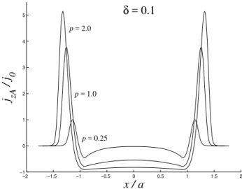
δ
= 0.1
Fig. 3. The spatial structure of the currentjzA(x)for a fixed spa-tial scaleaand smoothness parameterδ=0.1, for several values of
p=λA0/a.
From Eq. (9) one may obtain the relationship for the prop-agating Alfv´en waves (6) as follows:
jzA = ±6A(∇ ·E⊥)= ∓6A∇⊥2ϕ, (10)
where the upper/lower signs correspond to the upper/lower ARL boundary (because of the symmetric jump in the poten-tial across the layer).
The interaction of AI with the ARL can be categorized by the Alfv´en damping scaleλA=√6AQ/2, introduced by
Vogt and (1998), and Fedorov et al. (2001). This parameter is the scale of the flux tube where the field-aligned conductance matches the Alfv´en wave conductance. As the resistanceQ
of the ARL increases the parameterλAgrows larger.
5 Transverse spatial structure of Alfv´en impulse
We assume that the system under consideration is infinitely extended along they axis, similar to the auroral arc configu-ration. Equation (8) for the AI potential in a 1-D inhomoge-neous (alongxaxis) plasma is as follows:
ϕ′′−κ(x)2ϕ=j0/6A,
whereκ(x)2=λ−A2(x)=2/6AQ(x). For the profile ofQ(x)
with maximal valueQ0and transverse scalea (Fig. 2) this equation can be re-written as:
ϕ′′− κ
2 0
g(x/a)ϕ= j0
6A, (11)
where κ0=λ−A01=(2/6AQ0)1/2. The function
g(x/a)=Q(x)/Q0(0<g≤1)describes the transverse spatial structure of the ARL. Equation (11) can be normalized using the dimensionless variable ξ=x/a and the dimensionless potential u=ϕ/ϕ0, where ϕ0=j0Q0/2=j0/(6Aκ02), as
follows:
p2u′′−u/g(ξ )=1. (12)
−4 −3 −2 −1 0 1 2 3 4
−2 −1 0 1 2 3 4 5 6
x / a
j
zA/ j
0
p
= 2.0
δ = 0.1
δ = 0.25
δ = 0.5 δ = 1.0
Fig. 4.The structure of induced currentjzAfor certain fixed scale
aand parameterλA0(p=2.0) with respect to the parameterδ.
Here the parameterp=(κ0a)−1=λA0/ais the ratio between the characteristic Alfv´en damping scale and the ARL width. The induced electric fieldExand the induced field-aligned
current densityjzAcan be derived via the dimensionless
po-tentialu(ξ ):
Ex= −∂xϕ = −(ϕ0/a)∂ξu= −E0p∂ξu,
jzA = −6A∂xxϕ= −j0[1+u/g]= −j0p2∂ξ ξu. (13)
HereE0=ϕ0κ0=j0λA0/6A denotes the characteristic value
ofEx.
Let us suppose that the transverse profile of the ARL is described by an even functiong(ξ ), determined by the for-mulas:
g(ξ )=
1 at |ξ| ≤1−δ,
cosh−2[1+(|ξ| −1)/δ] at |ξ| ≥1−δ. (14)
The parameter δ(0<δ≤1) in Eq. (14) characterizes the smoothness of the ARL edges. Thus, whenδ=1 the profile is smooth, namelyg(ξ )=(coshξ )−2, whereas whenδ→0 the distribution tends to be step-wise (considered in the next sec-tion).
Equation (12) has been solved numerically as a bound-ary problem with a zero boundbound-ary condition at infinity for the chosen ARL profile (14). Figure 3 shows the calcula-tion results for the spatial structure of the currentjzA(x)for
a fixed spatial scaleaand smoothness parameter δ=0.1 for several values of the ARL resistance characterized by the ra-tio p=λA0/a. The induced current is concentrated at the ARL edges. Inside the ARL, a more widely distributed re-verse induced current flows which tends to compensate the background external current. The larger the resistance of the ARL, the bigger the amplitude will be of the excited current impulsejzA. For example,jzA/j0≃5 forp=2.0, but it drops tojzA/j0≃1 forp=0.25.
−6 −4 −2 0 2 4 6 −1
−0.5 0 0.5 1 1.5 2
x /
λ
Aj
zA/ j
0
0.5 1.0
2.0 5.0
δ
= 0.5
Fig. 5. The spatial structure of induced currentjzA(x)for a fixed characteristic lengthλA0with respect to the ARL width
character-ized byp(indicated near curves).
smoothness of the ARL edges characterized by parameterδ. Comparison of curves for variousδ shows that the sharper the ARL edges (the smallerδ), the larger the peak current density will be for the same ARL resistance (the samep). The peak current density can even exceed several times the density of the original currentj0, whenδ≪1.
Figure 5 shows the calculated spatial structure (in dimen-sionless variable x/λA0) of the induced current under the
fixed Alfv´en scaleλA0and ARL smoothnessδ=0.5, for sev-eral values ofp(i.e. for different scalesa). It follows from this plot that for the same magnetospheric parameters the peak intensity of the induced current increases with a de-crease of the ARL width (inde-crease ofp).
However, the integral induced current flowing into the ionosphere depends on the ARL scale in a different way as compared to the current densityjzA. The occurrence of the ARL causes the redistribution of the background external current in such a way that the total disturbed current vanishes, namely
Z
jzA>0
jzA(x) dx= − Z
jzA<0
jzA(x)dx.
The total current integrated over the regions with a positive current density actually is determined by the peak values of the induced electric fieldEx(x)in the ARL. Indeed, because
of the relation (10) and owing to the assumed symmetry of the model (so maxEx=−minEx), the total current is related
to maxExas follows: JzA =
Z
jzA>0
jzA(x) dx=26AmaxEx.
Figure 6 shows the structure ofEx(x)under fixedλA0 and
δ=0.5 for various scales a. Each curve is denoted by the relevant value ofp=λA0/a. The insert in Fig. 6 shows the
−10 −9 −8 −7 −6 −5 −4 −3 −2 −1 0 0
0.1 0.2 0.3 0.4 0.5
x /
λ
A
E
x/ E
0
0.1
0.125
0.25
0.5
1.0
2.0
5.0
δ
=0.5
0 2 4 6 8 10
0 0.1 0.2 0.3 0.4 0.5
a/λ
A
max
E
x
/ E
0
Fig. 6. The electric field along the ARL and the dependence of
maxExon the scalea.
dependence of maxEx in respect to a. As it can be seen
from this figure, the integrated currentJzA∝maxEx grows
(∝a) undera≪λA0, and gradually decreases at largea. The
maximal disturbance of total current is produced by the ARL with scalesa comparable to the Alfv´en damping scale, that isa/λA0∼1.
6 Structure of the Alfv´en impulse in a step-wise ARL
In a simplified case, corresponding to the elongated box-like profile of the ARL (δ→0), the AI spatial structure can be described analytically (Arykov and Maltsev, 1983). From Eq. (11) withg(ξ )=η(1−|ξ|), whereη(ξ )is the Heaviside’s function (η(ξ <0)=0 andη(ξ≥0)=1), the expression for po-tential follows
ϕ=ϕ0
cosh(κ0x)−cosh(κ0a) cosh(κ0a)
η(a− |x|).
The electric field in the ARL is
Ex= −∂ϕ ∂x =E0
sinh(κ0x) cosh(κ0a)
η(a− |x|).
The peak values of electric field are reached at the edges x= ± a: Ex(m)=|Ex(±)|=E0tanh(κ0a). For small-scale structures, a≪λA0, the peak value is
E(m)x ≃E0κ0a=j0a/6A. Disturbance of current is
jzA =6A ∂Ex
∂x = −j0
cosh(κ0x) cosh(κ0a)
η(a− |x|)
+j0 κ0
tanh(κ0a)[δ(x+a)+δ(x−a)],
−6 −4 −2 0 2 4 6 −0.8
−0.6 −0.4 −0.2 0 0.2 0.4 0.6 0.8
x / h
H
x/ H
(g)
0.25 0.5
1.0 2.0 3.0 4.0
δ
= 0.25
λ
A0
/
h
= 1.00
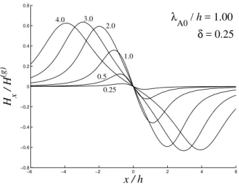
Fig. 7. The numerically calculated spatial structure of the ground magnetic response for several values ofα(indicated near curves) andλA0/ h=1.0.
within the ARL. The maximal value of the current distur-bance, j0 at x=±a, compensates for the background cur-rent. In the casea≫λA0, the region where the reverse
cur-rent is significant (jzA≃j0) is very narrow as compared to the
ARL widtha, whereas ata≪λA0, the reverse currentjzA≃j0 occurs throughout the entire ARL. The integrated current
JzA∝maxEx=E0tanh(a/λA0) grows in a monotonic way upon the increase of scale a, approaching the asymptotic value 26AE0.
7 Ground effect of the Alfv´en impulse
The ground effect of the 1-D AI-related currentjzA(x, t )is
produced by the ionospheric Hall current along they axis. This current is induced by theExcomponent of the incident
AI:
jH =
26H6A 6A+6P
Ex. (15)
Expression (15) is obtained using the boundary conditions upon reflection of an Alfv´en wave from the thin ionosphere with the height-integrated conductivities6H and6P.
The ground magnetic effect of the ionospheric Hall current (15) can be found using Biot-Savart’s law. Near the surface of the highly-conductive ground theHzcomponent vanishes and theHxcomponent doubles, so
Hx(x)= 4h c
∞
Z
−∞
jH(x′) dx′
h2+(x′−x)2, (16) whereh is the altitude of the conductive current above the Earth’s surface. The sign in Eq. (16) corresponds to the Northern Hemisphere.
In order to apply directly the estimates of the ground ef-fect of the solution for the dimensionless potentialu(ξ;p)of
Eq. (12), relationship (16) has been normalized by the scale
a. Introducing the parameterα=a/ h, that is the ratio be-tween the ARL width and the height of the ionosphere, this relationship can be presented as:
Hx(ξ;α, p)= −H(g) λ
A0
h 2 Z∞
−∞
∂ξ′u(ξ′;p) dξ′
1+α2(ξ′−ξ )2. (17) Here we have introduced a characteristic value of the ground magnetic fieldH(g)=86H(6A+6P)−1j0hc−1that does not depend on the parametersλA0anda and refers to the case when the three considered linear scales, λA0, a, andh, are
the same.
The spatial ground structure of the normalized magnetic disturbance Hx(x)/H(g) has been calculated numerically
and it is shown forδ=0.25 in Fig. 7 for several values ofα
and parameterλA0/ h=1.0. The ground magnetic signal has a bi-polar structure: it changes polarity beneath the ARL.
Geometrical attenuation of magnetic response upon trans-mission through the ionosphere is weak for large-scale struc-tures when α≥1 or a≥h. In this case the peak magnetic values Hx(m)=max|Hx|≃H(g). For example, in the case λA0/ h=1.0 at α=3.0 the peak value of the ground mag-netic disturbance is Hx(m)≃0.63H(g) (Fig. 7). The
atten-uation of the ground magnetic response from small-scale structures a≪h becomes significant. For example, for the same plasma parameters, Hx(m)≃0.36H(g) for α=1.0, and Hx(m)≃0.003H(g)forα=0.1.
Let us examine the attenuation of small-scale structures in greater detail. In the case of small-scale ARL as compared with the height of the ionosphere, i.e.α≪1, relationship (17) can be presented as the 2-D dipole approximation, namely
Hx(x)=16M hx
(h2+x2)2.
HereMis the magnetic moment per unit length along they
axis, created by the Hall currentjH, namely
M=1
2c
∞
Z
−∞
jH(x) xdx.
The maximum magnetic disturbance on the ground is achieved at the distancex(m)from the center of the ARL:
Hx(m) ≃3√3|M|h−2 at x(m) = ±h/√3. (18) The magnetic momentMmay be expressed via the normal-ized potentialu(ξ;p)<0 as follows:
M= −1
8λ 2
A0H(g)αU (p), U (p)= −
∞
Z
−∞
u(ξ;p) dξ .(19)
On the order of magnitude,U≃max|u|, because the inte-grand functionu(ξ )is exponentially small beyond the unit-length interval.
Now we consider the dependence of the integral function
a. It follows from the analysis of the boundary problem for Eq. (12) that when ARL is wide (p≤1), the value ofU (p)≃1. When the ARL is narrow (p≫1), the valueU (p)becomes as small asU (p)∼p−µ, withµin the interval 0<µ≤2. The power factorµdepends on the parameterδ. It is easy to find
µanalytically for the step-wise ARL profile (δ→0). In this case atp≫1 the functionu(x;p)≃12p−2(x2−1)η(1−|x|), and thereforeM(p)≃23p−2, that isµ=2. Numerical calcu-lations show that the factorµdecreases somewhat for more smooth ARL edges. For example, atδ=0.05 it is quite close to the “step-wise” value: µ=1.87, whereas atδ=0.25 this factorµ=1.47.
For a narrow ARL (α≪1), two cases are possible depend-ing on the ratio between the characteristic lengthλA0andh. IfλA0≪h, then
Hx(m)
H(g) ≃
(λA0/ h)2(a/ h) at a ≥λA0,
(λA0/ h)2−µ(a/ h)1+µ at a≪λA0. (20) One can see from the above estimate that the maximum mag-netic field decays linearly upon the decrease of the scalea, and only whena become smaller thanλA0does this decay occur faster, by a power lawa1+µ (e.g. cubic for the step-wise profile).
IfλA0≥h, then underα≪1 there is only the possible lim-iting casea≪λA0, when the peak ground magnetic
distur-bance Hx(m)/H(g) is described by the second relationship
from Eq. (20). The above consideration indicates that the ground magnetic disturbance produced by small-scale struc-tures, α≪1, in some cases decreases not as fast upon the decrease of the ARL scalea.
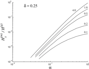
The analytical estimates are confirmed by the numerical calculations of dependenceH(m)(α). Figure 8 shows the de-pendence of normalized peak values of ground magnetic dis-turbance,H(m)/H(g), with respect toαfor several values of
λA0/ h(indicated near curves) for the same smoothness pa-rameterδ=0.25 as in Fig. 7. It can be seen that upon the decrease ofα the rate of magnetic field decrease is rather slow (nearly linear) in the range of parametersλA0/ h≤0.2 and α≥0.2, and faster for α≤0.2 (power law with factor ∼2.47). The examination of Fig. 8 shows that the ground magnetic response from small-scale ARL is essentially at-tenuated. However, this attenuation is not so severe (about an order of magnitude only) in the range of parametersα≥0.2 andλA0/ h≥0.5 to prevent the ground observations of the ARL-related AI in some situations.
8 Model consequences and comparison with observa-tions
At the initial phase of the reconfiguration of global currents in the nightside magnetosphere during substorm onset, the ionosphere plays a role as only a passive sink of energy for the magnetospheric field-aligned current. Only when this current exceeds a certain threshold does an anomalous resis-tivity emerge on auroral field lines. In the region of upward
10−2 10−1 100
10−4 10−3 10−2 10−1 100
α H x
(m)
/ H
(g)
0.1 0.2 0.5 1.0 4.0
δ = 0.25
Fig. 8. The numerically calculated dependence of the normalized
ground magnetic response peak values onαfor several values of
λA0/ h(indicated near curves) andδ=0.25.
current, the moment of an anomalous resistance and elec-tric field emergence, as described in Sect. 1, indicates the onset of positive feedback in the magnetosphere-ionosphere system. However, the situations when the considered mech-anism can be operative may occur not only during the main onset but during any intensification of field-aligned current of sufficient magnitude and accompanying auroral activation.
Many global observational campaigns (Yumoto et al., 1990; Yeoman et al., 1991; Uozumi et al., 2000, 2004) show that Pi2 is a global phenomenon which is observed over a wide range of latitudes (until the equatorial latitudes) and LT, even till the dayside (Sutcliffe and Yumoto, 1991). There-fore, a global compressional mode should be involved in the excitation of Pi2. This large-scale compressional mode is probably generated by bursty processes during substorm on-set in the nightside magnetosphere. Upon propagation to-wards the inner magnetosphere this mode illuminates the whole nightside magnetosphere and can be transformed on Alfv´en velocity gradients into transient Alfv´en oscillations (Baransky et al., 1980). When the field-aligned current den-sity at the front of the disturbance generated by the sub-storm detonation exceeds the threshold sufficient for the ex-citation of some high-frequency turbulence (most probably at altitudes about 1RE), an anomalous resistivity is turned
on. This moment is to be accompanied by the excitation of additional local transient AI, as was indicated by Arykov and Maltsev (1983). The theoretic model presented here de-scribes the features of this impulse.
1330 1335 1340 1345 1350 -200
-150 -100 -50 50
KTN
TIK
CHD Raw Data
CPMN data / Jan. 3, 1997
UT 1333:37-1334:04
0
H D
-40 -20 0 20 40
1330 1335 1340 1345 1350
UT
Filtered Data [40-100s] H D
KTN
TIK
CHD
Fig. 9. Magnetic intensification and Pi2 transients, recorded at
CPMN stations on 3 January 1997. The vertical lines indicate the moments of the auroral intensifications observed by Polar UV im-ager.
to the ground ULF disturbance during a substorm break-up can be done with a more dense array of magnetometers with high time resolution. Special methods of analysis are neces-sary to discriminate contributions from various mechanisms into Pi2 signature. For example, to reveal a fine temporal structure of Pi2 trains, the phase breaks in their wave forms can be used as time markers for abrupt processes in the FAC signatures.
The occurrence of the AI described above should coincide with a brightening of an auroral arc due to additional accel-eration of auroral electrons by the anomalous electric field. However, the delay of a few tens of seconds is possible, ow-ing to the difference in the electron and MHD transit times. The model considered predicts an excitation of a very spa-tially localized response, because no compressional mode is generated during the anomalous resistance onset.
8.1 Estimates of critical plasma parameters and AI peak magnitudes
Let us estimate the expected parameters of the AI related to the ARL emergence. The threshold for the excita-tion of plasma instabilities and related anomalous resistance by the field-aligned current is different for different types of turbulence. It is highest for the Buneman instability
j∗≃enue≃5·10−5A/m2, it is lower for the ion-sound in-stabilityj∗≃enus≃10−5A/m2, and it is even lower for the ion-cyclotron instability ∼5·10−6A/m2 (Kindell and Ken-nel, 1971). Thresholds values for all these instabilities have a deep and narrow minimum at altitudes∼103−3·103km, where the formation of ARL could be expected. The iono-spheric projection of the ARL is about the width of the auro-ral arc. The ARL width, as well as the auroauro-ral arc thickness, may vary over a wide range, from fractions of km to hun-dreds of km.
The Alfv´en damping scaleλA0is mainly determined by a magnitude of the anomalous resistivity. However, estimates ofσk, being very uncertain, may vary in a wide range. Nu-merical modeling by Strelzov and Lotko (2003) of Alfv´en wave interaction with the ARL demonstrated a significant wave reflection with transverse scales∼20 km. We suppose that this scale should coincide withλA0.
The following order-of-magnitude estimates of possible peak values can be obtained from the above formulas for the east-west elongated ARL. The transverse radial electric field of the AI isE≃E0≃j0λA06A−1, and corresponding azimuthal magnetic component is B≃(c/VA)E0=4πj0λA0c−1. The drop in the potential across the ARL is{ϕ}≃2ϕ0=j0Q. The induced field-aligned current density is comparable to the ini-tial global current densityjzA≃j0. The disturbance of total current isJ≃26AE0=2j0λA0. The ground disturbance has a bipolar latitudinal structure with a phase reversal just be-neath the ARL ionospheric projection. If the ARL is wide, as compared with the ionospheric height (a≥h), the iono-sphere does not produce substantial geometric attenuation of the magnetic impulse. However, even if the ARL is narrow (a≪h), in the caseλA≪h, this attenuation is not
dramati-cally large, and the ground magnetic response could possibly be revealed from ground magnetograms. The peak ground signal is
H(m) ≃H(g) λ
A0
h 2
= 686H A+6P
λ2A0j0
ch .
These peculiarities may help to discriminate this impulse from the transient responses produced by other mechanisms, such as a burst of precipitating electrons, or cross-tail current disruption.
1332: 23 UT
L B HL
1332: 50 UT
L B HL
1333: 37 UT
L B HS
1334: 04 UT
L B HS
1335: 27 UT
L B HL
1335: 54 UT
L B HL
1336: 41 UT
L B HS
1337: 08 UT
L B HS
P olar Ultraviolet Imager
Day 003 01/03 1997
P hotons -c m-2-s-1
0 2 4 6 8 10 12 14
Fig. 10
Fig. 10.The snapshots of UVI (LBHL) aurora made by Polar on 3 January 1997.
TIK KTN
CHD
Fig. 11. The mapping of Polar UVI image onto the position of
CPMN stations in Northern Russia at 3 January 1997, 13:38:22 UT (in geomagnetic coordinates).
these field lines, the disturbance caused by the excited AI decays fast, and more simple waveforms can be observed.
It is necessary to indicate that we have considered here the non-consistent problem – the onset ofσk under steady
j0, owing to fluctuations of plasma parameters near the threshold (that is, the external turn-on). To elucidate fully the physics of AI, an additional problem should be analyzed: a self-consistent description of theσkonset by a time-increasingj0. Elsewhere, we are going to consider this self-consistent problem.
A detailed consideration of the further evolution of the ex-cited AI is beyond the scope of this paper. Transient AI will interact with the ionosphere and the ARLs in the Northern and Southern hemispheres. Upon this interaction parts of the incident wave energy are reflected and absorbed by ARL, and part penetrates through the ARL (Lysak and Dum, 1983; Trakhtenhertz and Feldstein, 1985). As a result, some part of the AI energy will be trapped in the Alfv´en quasi-resonator between the conjugate ARLs, and part will be trapped in the cavity between the ionosphere and the ARL (Pilipenko et al., 2002; Streltsov and Lotko, 2003). If the reflection from the ARL does occur, the period of transient response to the ex-cited Alfv´en impulse will be shorter than the fundamental eigenperiod of the same field line.
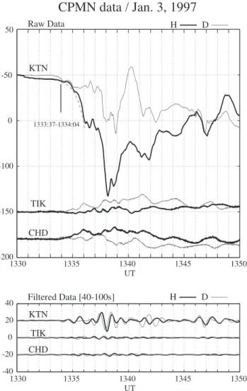
9 Event on 3 January 1997
As a qualitative illustration of the principal feasibility of the considered effect, we consider the event on 3 January 1997. This substorm-like intensification with an amplitude of about 100 nT has been detected by stations from the Circum-Pacific Magnetometer Network (CPMN) at 13:30– 13:50 UT (Fig. 9): Kotelny (KTN, geomagnetic coordinates: 69.9◦, 201.0◦, L=8.5, MLT≃UT+16), Tixie (TIK, 65.7◦, 196.9◦, L=5.9, MLT≃UT+16), and Chokurdakh (CHD, 64.8◦, 212.4◦, L=5.6, MLT≃UT+15). A decrease in the magnetic field H component started at 13:31 UT. However, at 13:34 UT the rate of the magnetic field decrease rapidly changed. The trend of the development of the bay is drawn as a dashed curve. This moment coincided with the auroral UVI intensification as observed by the Polar satellite (Fig. 10). Another rapid change of the magnetic field decrease and au-rora intensification occurred at 13:37 UT.
Band-pass filtering (40–100 s) indicates the occurrence of Pi2-like oscillations at KTN with a period of about 1 min and a peak-to-peak amplitude∼10 nT.
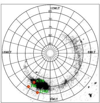
The mapping of the Polar UV image, corresponding to the moment 13:38 UT just after the aurora intensification, onto the CPMN stations positions, shown in Fig. 11, indicates that only KTN was beneath the arc intensification region, whereas the stations TIX and CHD were beyond it, though not very far. As Fig. 9 shows, the Pi2-like signals were de-tected at KTN only, at TIK their amplitudes did not exceed 1 nT. Thus, the ground transient response is highly localized within the region of the aurora intensification.
At the recovery phase of this bay, Pc5 oscillations with a period∼2.5–3.0 min were observed (Fig. 9). The period of these oscillations probably corresponds to the fundamental eigenperiod of the field line. Thus, the Pi2 period is shorter than the expected fundamental eigenperiod.
The basic features of this event agree with the scenario of a two-phase substorm development and the predictions of the AI generation model. However, the given example was in-tended to show the occurrence of localized Pi2-like response, and spatial and temporal correspondence between the mag-netic transients and auroral activation, but it cannot be con-sidered as firm evidence in favor of the suggested mecha-nism. The auroral bulge as seen in the Polar image may com-prise many discrete auroral arcs, each with an individual time evolution and its magnetic fingerprint. To discriminate con-tributions to ground magnetic response from different source mechanisms during a substorm onset or auroral activation it is necessary to have a more dense (than CPMN) network of magnetic stations and auroral observations with a higher spa-tial resolution.
10 Conclusion
Following the idea of Arykov and Maltsev (1983), we have shown that the onset of anomalous resistance on auroral field lines is accompanied by the excitation of an AI. The gener-ated AI indicates the transition of the global magnetosphere-ionosphere instability into an explosive phase with a posi-tive feedback. The spatial structure of this impulse, both in space and on the ground, has been described both analyt-ically and numeranalyt-ically under the thin layer approximation. The field-aligned current transported by the Alfv´enic impulse is concentrated near the edges of the layer with anomalous resistivity, whereas the reverse currents are spread over the layer. According to our estimates, the AI amplitude may be sufficient to be detected by ground magnetometers under fa-vorable conditions. Observations indicate that this mecha-nism may be responsible for some Pi2-like wave transients detected during an auroral activation.
Acknowledgements. The Polar data were provided by C. Meng and K. Liou from the Johns Hopkins University, Applied Physics Labo-ratory.
We appreciate the helpful comments of both reviewers. This re-search is supported by the fellowship from Heiwa Foundation (VA),
INTAS grant 03-05-5359 (NM), and RFBR grant 03-05-64670 (EF).
Topical Editor T. Pulkkinen thanks T. B¨osinger and another ref-eree for their help in evaluating this paper.
References
Arykov, A. A. and Maltsev, Yu. P.: Generation of Alfv´en waves in an anomalous resistivity region. Planet. Space Sci., 31, 267–273, 1983.
Baumjohann, W. and Glassmeier, K. H.: The transient response mechanism and Pi2 pulsations at substorm onset – Review and outlook, Planet. Space Sci., 32, 1361–1370, 1984.
Baransky, L. N., Sterlikova, I. V., Troitskaya, V. A., Gokhberg, M. B., Pilipenko, V. A., and Munch, J.: Investigation of Pi2 pulsa-tions along geomagnetic meridian, I. Meridional distribution of intensity and spectral content, Geomagn. Aeronomy, 20, 896– 904, 1980.
Belyaev, P. P., B¨osinger, T., Isaev, S. V., and Kangas, J.: First ev-idence at high latitudes for the ionospheric Alfv´en resonator, J. Geophys. Res., 104, 4305–4317, 1990.
Fedorov, E., Pilipenko, V., and Engebretson, M. J.: ULF wave damping in the auroral acceleration region, J. Geophys. Res., 106, 6203–6212, 2001.
Groot-Hedlin, C. D. and Rostoker, G.: Magnetic signatures of pre-cursors to substorm expansive phase onset, J. Geophys. Res., 92, 5845–5856, 1987.
Kepko, L., and Kivelson, M. G.: Generation of Pi2 pulsations by bursty bulk flows, J. Geophys. Res., 104, 25 021–25 034, 1999. Kepko, L., Kivelson, M. G., and Yumoto, K.: Flow bursts, braking,
and Pi2 pulsations, J. Geophys. Res., 106, 1903–1915, 2001. Kindel, J. M. and Kennel, C. F.: Topside current instabilities. J. Geophys. Res., 76, 3055, 1971.
Liou, K., Meng, C.-I., Lui, A. T. Y., Newell, P. T., Brittnacher, M., Parks, G., Reeves, G. D., Anderson, R. R., and Yumoto, K.: On relative timing in substorm onset signatures, J. Geophys. Res., 104, 22 807–22 817, 1999.
Liou, K., Meng, C.-I., Newell, P. T., Takahashi, K., Ohtani, S.-I., Lui, A. T. Y., Brittnacher, M., and Parks, G.: Evaluation of low-latitude Pi2 pulsations as indicators of substorm onset using Po-lar ultraviolet imagery, J. Geophys. Res., 105, 2495–2505, 2000. Lui, A. T. Y.,: Current disruption in the Earth’s magnetosphere: Observations and models, J. Geophys. Res., 101, 1 067–13 088, 1996.
Lysak, R. L. and Dum, C. T.: Dynamics of magnetosphere-ionosphere coupling including turbulent transport, J. Geophys. Res., 88, 365–380, 1983.
Lysak, R. L. and Song, Y.: Energetics of the ionospheric feedback interaction, J. Geophys. Res., 107, 1160, doi:10.1029/2001JA000308, 2002.
Maltsev, Yu. P., Leont’ev, S. V., and Lyatsky, V. B.: Pi2 pulsations as a result of evolution of an Alfv´en impulse originating in the ionosphere during a brightening of aurora, Planet. Space Sci. 22, 1519–1523, 1974.
Olson, J.V.: Pi2 pulsations and substorm onsets: A review, J. Geo-phys. Res., 104, 17 499–17 520, 1999.
Pilipenko, V., Fedorov, E., and Engebretson, M. J.: Alfv´en res-onator in the topside ionosphere beneath the auroral acceleration region, J. Geophys. Res., 107, SMP22 1–10, 2002.
Feed-back instability, J. Geophys. Res., 106, 25 813–25 824, 2001. Shiokawa, K., Baumjohann, W., Haerendel, G., et al.: High-speed
ion flow, substorm current wedge, and multiple Pi2 pulsations, J. Geophys. Res., 103, 4491–4508, 1998.
Shiokawa, K., Yumoto, K., and Olson, J. V.: Multiple auroral brightenings and associated Pi2 pulsations, Geophys. Res. Lett., 29, doi:10.1029/2001GL014583, 2002.
Streltsov, A. V. and Lotko, W.: Reflection and absorption of Alfv´enic power in the low-altitude magnetosphere, J. Geophys. Res., 108, 8016, doi:10.1029/2002JA009425, 2003.
Sutcliffe, P. R. and Yumoto, K.: On the cavity mode nature of low-latitude Pi2 pulsations, J. Geophys. Res., 96, 1543–1551, 1991. Trakhtenhertz, V. Yu. and Feldstein, A. Ya.: About dissipation of
Alfv´en waves in the layer with anomalous resistance, Geomag. Aeronomy, 25, 334–336, 1985.
Trakhtengertz, V. Yu. and Feldstein, A. Ya.: Auroral ionosphere electrodynamics during the switch-on of the energetic particles source, Geomag. Aeronomy, 28, 598–605, 1988.
Uozumi, T., Yumoto, K., Kawano, H., Yoshikawa, A., Ol-son, J. V., Solovyev, S. I., and Vershinin, E. F.: Charac-teristics of energy transfer of Pi2 magnetic pulsations: Lat-itudinal dependence, Geophys. Res. Lett., 27, 1619–1622, doi:10.1029/1999GL010767, 2000.
Uozumi T., Yumoto, K., Kawano, H., et al.: Propaga-tion characteristics of Pi2 magnetic pulsaPropaga-tions observed at ground high latitudes, J. Geophys. Res., 109, A08203, doi:10.1029/2003JA009898, 2004.
Vogt, J. and G. Haerendal: Reflection and transmission of Alfv´en waves at the auroral acceleration region, Geophys. Res. Lett., 25, 277–280, 1998.
Yeoman, T. K., Milling, D. K., and Orr, D.: Polarization, propaga-tion and MHD wave modes of Pi2 pulsapropaga-tions: SABRE/SAMNET results, Planet. Space Sci., 39, 983–998, 1991.