Economic Activity in Brazil After the Real
Plan: Stylized Facts from SVAR Models
∗
Brisne Céspedes
†
, Elcyon Lima
‡
, Alexis Maka
§
Contents:1. Introduction; 2. Brazilian Stylized Facts and VARs: A Brief Review of the Literature; 3. Data and Estimation Procedures; 4. “Contemporaneous Causation” and the Identification of Structural VARs;
5. Causal Inference and the Identification of Structural VARs; 6. Monetary Policy Developments since
the Real Plan; 7. Basic Model and Results for the First Subsample (1996:07-1998:08); 8. Basic Model
and Results for the Second Subsample (1999:03-2004:12); 9. Concluding Remarks.
Keywords:Structural VAR; Monetary Policy; Directed Acyclic Graphs.
JEL Code:E31; C32.
Este artigo obtém alguns fatos estilizados sobre as flutuações de curto prazo da economia brasileira após o Plano Real, dando atenção especial à identificação dos efeitos dos choques da política monetária. Dadas as al-terações na política monetária, ocorridos após o Plano Real, optamos por dividir a nossa análise em dois subperíodos (1996:07-1998:08 e 1999:03-2004:12). Os modelos de Auto-Regressão Vetorial Estrutural (SVAR) foram identificados através do uso de grafos acíclicos direcionados. Em contraste com a maioria das análises feitas para o Brasil, que adotam modelos SVAR, encontramos evidências de que uma política monetária contracionista re-duz o nível geral de preços.
This article uncovers some stylized facts about the short run fluctuations of the Brazilian economy after the Real Plan, giving special attention to the iden-tification of the effects of monetary policy shocks. A distinctive feature of this article is the careful attention paid to monetary policy developments after the Real Plan when dividing our sample into two subsamples (1996:07-1998:08 and
∗Financial support from REDE-IPEA is gratefully acknowledged. The views expressed in this paper are those of the authors and do not necessarily represent those of the IPEA or the Brazilian Ministry of Strategic Affairs.
†Instituto de Pesquisa Econômica Aplicada (IPEA), Av. Presidente Antônio Carlos, 51 / 15o andar, Rio de Janeiro, RJ, Brazil. E-mail:
‡Instituto de Pesquisa Econômica Aplicada (IPEA) and Universidade Estadual do Rio de Janeiro (UERJ). E-mail: elcyon. [email protected]
§Instituto de Pesquisa Econômica Aplicada (IPEA), Av. Presidente Antônio Carlos, 51 / 15o andar, Rio de Janeiro, RJ, Brazil. E-mail:
124
Brisne Céspedes, Elcyon Lima e Alexis Maka
1999:03-2004:12). We use directed acyclic graphs to identify the Structural Vector Autoregression (SVAR) models. In contrast with most SVAR analysis for Brazil, we found empirical evidence that supports the view that a contractionary mon-etary policy indeed reduces the price level.
1. INTRODUCTION
This article investigates the stochastic and dynamic relationship of a group of Brazilian macroeco-nomic variables (price and industrial production indexes, nominal exchange rate, short and medium-run nominal interest rates, money, and international reserves) for the period after the Real Plan (1996 - 2004). We adopt, as has become usual in the literature, several SVARs (Structural VARs) models to uncover stylized facts about the short-run impacts of the identified exogenous sources of fluctuations of this selected group of variables, with emphasis on the identification of the effects of monetary policy shocks. Structural inference and policy analysis employing VARs require differentiating between corre-lation and causation, an issue known as “the identification problem”. The practice in the literature has been to use identifying assumptions based on “economic theory” or institutional knowledge to sort out the contemporaneous links among the variables in order to allow correlations to be interpreted causally. Unfortunately, the literature has not yet agreed on a particular set of assumptions for identifying the effects of exogenous shocks to monetary policy.
The choice of identification strategy for monetary policy shocks is still an unresolved dispute in macroeconomics.
There are many recent empirical studies about the dynamic relationship of sets of macroeconomic variables in country-regionBrazil employing SVARs as the framework of their analysis (Fiorencio et al. (1998), Rabanal and Schwartz (2001), Arquete and Jayme Jr. (2003), and Minella (2003), among others). With the exception of Fiorencio et al. (1998), all of them use Cholesky decompositions of the covari-ance of reduced form VAR disturbcovari-ances to identify the model. What distinguishes our article from the existing Brazilian literature is the adoption of a procedure that, under certain assumptions regarding the underlying data generating process, uses statistical properties of the sample – more specifically, conditional independence relations between the variables – to select over-identifying restrictions to estimate the SVARs. These restrictions follow from directed acyclic graphs (DAGs) estimated by the TETRAD software developed by Spirtes et al. (1993, 2000) using as input the covariance of reduced form VAR disturbances. Another distinguishing characteristic of our article is the careful attention paid to monetary policy developments after the Real Plan in the selection of appropriate subsamples. The first subsample goes from 1996:07 to 1998:08, the period with exchange rate “mini-bands” combined with the adoption of the TBC rate as an informal target for the SELIC rate. The second subsample goes from 1999:03 to 2004:12, the period with free-floating exchange rate and explicit SELIC targeting.
Over the last years there has been a growing interest on graphical models and in particular on those based on DAGs as a general framework to describe and infer causal relations, exploring the connection
between causal structure and probability distributions.1 These methods have been used in a variety of
fields but are unfamiliar to most economists. Swanson and Granger (1997) were the first to apply graph-ical models to identify contemporaneous causal order of a SVAR, although they restrict the admissible structures to causal chains. Bessler and Lee (2002) use error correction and DAGs to study both lagged and contemporaneous relations in late 19th and early 20th century U.S. data. Demiralp and Hoover (2003) evaluate the PC algorithm employed by TETRAD in a Monte Carlo study and conclude that it is an effective tool of selecting the contemporaneous causal order of SVARs. Awokuse and Bessler (2003) use DAGs to provide over-identifying restrictions on the innovations from a VAR and compare their results
1See for example, Spirtes et al. (1993, 2000), Pearl (2000), and Lauritzen (2001). For a critical evaluation of the use of graphs for
inferring causality see Humphreys and Freedman (1996, 1999).
with the ones of Sims (1986). Moneta (2004) use DAGs and the data set of Bernanke and Mihov (1998) to identify the monetary policy shocks and their macroeconomic effects in the U.S.. However, as we dis-cuss later on section 5, the use of DAGs for making causal inferences is subject to an important caveat: as Robins et al. (2003) have shown, causal procedures based on associations of non-experimental data
under weak conditions2, are not uniformly consistent. That means that for any finite sample, there are
no guarantees that the results of the causality tests will converge to the asymptotic (correct) results.3
In contrast with most of the VAR analysis of monetary policy shocks for Brazil, we found empirical evidence that supports the view that contractionary monetary policy shocks indeed reduce the price
level.4 The main results of our basic model are: i) In response to a contractionary short run interest
rate innovation, during the 1999-2004 subperiod, the exchange rate appreciates, the output and the price level decrease. However, the output response is faster and the price level responds with a lag of near six months in the basic model; ii) For the 1996-1998 subperiod, the most likely effect of a contractionary short run interest rate innovation is the reduction of the price level, even though there is a large uncertainty in this response, and the reduction of output; iii) Exogenous shocks to the exchange rate are, for the 1999-2004 period, the most important source of inflation rate fluctuation.
The article is organized as follows. Section 2 presents a brief review of the Brazilian literature on macro variables and VARs. Section 3 describes the data and the estimation procedures used. Section 4 explains how the identification of contemporaneous causation allows the identification of VARs. Section 5 shows how the Spirtes-Glymour-Scheines Model can be used to identify the SVARs. Section 6 describes monetary policy developments that followed the Real Plan. Sections 7 and 8 present the basic model and results for the first and the second subsamples, respectively, with section 8 discussing the results of an alternative model that includes money. Finally, we offer some concluding remarks on section 9.
2. BRAZILIAN STYLIZED FACTS AND VARS: A BRIEF REVIEW OF THE LITERATURE
In this section we present a brief review of the recent Brazilian literature related to VARs and groups of macroeconomic variables.
Within the classical approach to VARs we have the studies of Rabanal and Schwartz (2001), Arquete and Jayme Jr. (2003), and Minella (2003), while Fiorencio et al. (1998) use a Bayesian VAR (BVAR) in their analysis.
Fiorencio et al. (1998) use BVAR models to analyze the impacts of monetary and exchange rate poli-cies on unemployment and the price level after the Real Plan. The basic model was estimated for the period between January 1991 and May 1997, with and without intervention on July and August 1994, using as variables the price level (IPCA), the unemployment rate, the exchange rate, the interest rate over capital financing (“capital de giro”), and the spread between capital financing and private bonds (CDBs) rates. Employing a non-recursive identification they find that exchange rate shocks have signi-ficative impacts over the price level and unemployment, and that monetary policy shocks do reduce the
price level and increase unemployment (in the model with intervention).5 According to them the
re-sults suggest that there has been a change of regime after the Real Plan and that the effects of economic policy shocks in the model are sensitive to the way this change of regime is represented.
Rabanal and Schwartz (2001) use a VAR to analyze the effectiveness of overnight interest rate (SELIC) as a monetary policy instrument in Brazil and its effects on other interest rates, output, and prices
2These weak conditions are the Markov and faithfulness assumptions, which are defined on section 5.
3However, it has been shown that under stronger assumptions the procedures for inferring causality based on DAGs are
uni-formly consistent. See Zhang (2002), Zhang and Spirtes (2003).
4None of our results hinge on the use of DAGs or Tetrad to identify the VARs. They may be reproduced by ordinary identification
schemes, like the Cholesky decomposition of the covariance matrix.
126
Brisne Céspedes, Elcyon Lima e Alexis Maka
for the period between January 1995 and August 2000. The variables included in the VAR are real output, inflation (IPCA), SELIC rate, lending spreads, and money (M1), used in this order in the recursive
(Cholesky) decomposition of the variance-covariance matrix of errors.6 They conclude that the SELIC
rate has a significant and persistent effect on output and lending spreads but interest rate shocks seemed to increase inflation (“price puzzle”).
Arquete and Jayme Jr. (2003) evaluate the impact of monetary policy on inflation and output, cov-ering the period between July 1994 and December 2002. As variables of the model they used inflation
(IPCA), SELIC rate, and output gap, employed in this order in the recursive decomposition of errors.7
In some of their analysis they also included a fifth variable (alternatively the nominal exchange rate, the real exchange rate, and the international reserves at the Central Bank) intended to capture external constraints in Brazil. According to them monetary policy have real effects, external restrictions and exchange rate volatility are important to the Central Bank reaction function but interest rate shocks increase inflation.
Minella (2003) investigates the macroeconomic relationships involving output, inflation, interest rate, and money, comparing three different periods: January 1975 – July 1985, August 1985 – June 1994, September 1994-December 2000. His basic model includes output, inflation (IGP-DI), nominal interest rate (SELIC rate), and money (M1), used in this order in the Cholesky decomposition. His main results are that monetary policy shocks have significant effects on output but are not able to induce a reduction of inflation, with evidence suggesting the price puzzle in the second sub-period. For the Real Plan period, the results about the effects of monetary policy shocks over inflation are not conclusive.
More recently we have the contributions of Sales and Tannuri-Pianto (2005) and Fernandes and Toro (2005). Sales and Tannuri-Pianto (2005) apply for Brazil the Bernanke and Mihov (1998) methodology that imposes contemporaneous identification restrictions on a set of variables relevant to the market for commercial bank reserves in order to identify monetary policy shocks. Despite the uncertainty asso-ciated with their results, all their models displayed an inflation rate puzzle where the rate of change of the price level decreased temporarily in response to an expansionary monetary policy shock, although its effect over the price level is permanent. Fernandes and Toro (2005) estimate the monetary transmis-sion mechanism for Brazil after the Real Plan using a cointegrated VAR model, identifying the cointe-grated vectors as equilibrium relationships. They analyze the period from November 1994 to February 2001 as a whole, despite the change in the exchange rate regime that occurred on January 1999, treat-ing changes in international reserves and exchange rate as exogenous variables. Accordtreat-ing to their results, positive monetary policy shocks, identified as SELIC innovations, have a temporary, short-lived negative effect over the inflation rate, which disappears after six months, implying a permanent effect of monetary policy over the price level.
3. DATA AND ESTIMATION PROCEDURES
The models were estimated using monthly data divided into two subsamples: the first goes from
1996:07 to 1998:08 and second from 1999:03 to 2004:12.8The following variables were used: the SELIC
interest rate (adjusted average rate of daily financing guaranteed by federal government securities, calculated in the Special Settlement and Custody System (SELIC) and published by the Central Bank of Brazil, annualized rate); the nominal exchange rate (end of period buying rate – source: BCB); the IPCA (official price index used for targeting inflation – source: IBGE); the 180 days Swap rate (PRE x CDI - annualized rate considering 252 working days – the original source is the Brazilian Mercantile &
6Another ordering is also analyzed: SELIC rate, lending spreads, output, inflation, and money, but the results do not change
much.
7An alternative order analyzed was: output gap, inflation, SELIC rate.
8The reasons for splitting the sample into two subsamples and the particular choice of dates are based on monetary policy
developments after the Real Plan and are discussed on section 6.
Futures Exchange but the information that we used was collected from http://www.risktech.com.br/); the Industrial Production index, used as a proxy for output (source: IBGE); net foreign reserves (liquidity concept, as measured by the BCB); and a monetary aggregate (M1, working days average).
The VAR reduced forms were estimated equation by equation using ordinary least squares (OLS). Following the results of Sims and Uhlig (1991) and Sims et al. (1990), we do not performed unit root tests or cointegration analysis.9
4. “CONTEMPORANEOUS CAUSATION” AND THE IDENTIFICATION OF STRUCTURAL VARS
4.1. The Reduced Form VAR Model
Letxtbe the data vector – there are 5 variables in the model, thereforexthas dimension 5x1 – for
each period t : xt = [rtetptrstYt]′, where: rt= Selic rate;et= exchange rate ; pt= IPCA index;
rst= swap rate (180 days) ;Yt= industrial production index.
The reduced form VAR model is given by the following set of equations:
B(L)xt=µ+φZt+νt (1)
νt∼N(0,Σ)andE(νtνs′) = 0,∀t6=s
where:
B(L) =I−Pp
i=1BiLiandLis the lag operator;
Zt= seasonal dummies vector;
νt= reduced form residuals; andµ= constants’ vector.
This representation of the model does not allow for the identification of the effects of exogenous independent shocks to the variables since the VAR reduced form residuals are contemporaneously
cor-related (theΣmatrix is not diagonal).10 That is, the reduced form residuals(νt)can be interpreted
as the result of linear combinations of exogenous shocks that are not contemporaneously (in the same instant of time) correlated. It is not possible to distinguish whose exogenous shocks affect the residual of which reduced form equation. The residual can be the result, for example, of an exogenous and in-dependent shock to the exchange rate, an exogenous and inin-dependent shock to the interest rate, or a linear combination of both shocks. In evaluations of the model (and of economic policies) it only makes sense to measure exogenous independent shocks. Therefore, it is necessary to present the model in another form where the residuals are not contemporaneously correlated. A VAR where the residuals are not contemporaneously correlated is called a structural VAR and some of its equations have, in general, a behavioral interpretation. The same is not true for reduced form VARs.
4.2. The Structural Form VAR Model
The model in structural form is given by:
A(L)xt=ρ+θZt+ǫt (2)
ǫt∼N(0, D), D(diagonal) eE(ǫtǫ
′
s) = 0,∀t6=s
9They show that the classical unit roots asymptotics is of little practical value and that the common practice of attempting to
transform models into a stationary form by difference or cointegration operators, whenever it appears likely that the data are integrated is in many cases unnecessary.
128
Brisne Céspedes, Elcyon Lima e Alexis Maka
whereρ=A0µ, θ=A0φ, A(L) =A0B(L), ǫt=A0νt, A0is a full rank matrix with each element in
its main diagonal equal to one.
The relationships between the residualsǫtandνt, and the covariancesDandΣ, are given by:
νt=A(0)−1ǫtor alternatively,νt= [I−A0]νt+ǫt (3)
A0ΣA′
0=D (4)
Given an estimate ofA0 it is possible to estimate structural form parameters from estimates of
reduced form parameters. When the reduced form VAR is estimated restricting only the number of lags (chosen as the same in all equations and for all variables), with no further restrictions, the structural
VAR estimation proceeds in two steps.11 In the first step the reduced form VAR is estimated and this
comprise the estimation of the equation’s coefficients and of the covariance matrix of the reduced form
residuals(Sigmaˆ ). In the second step the matricesA0andDare estimated using only the information
given by the estimate of the covariance matrix of reduced form residuals (estimated in the first step).
There are in general a large number of full rank matricesA0andD(Ddiagonal) that allow us to
reproduceΣˆ. That is, there are several conditional dependency and independency contemporaneous
re-lations (“Markov kernels”) between the variables – given by different specifications of which parameter
inA0is free and which is equal to zero – that allow us to reproduce the partial correlations observed
for the reduced form residuals.12 In order to estimate the structural model it is necessary to identify a
number of conditional independence relations (that is, parameters equal to zero inA0) to satisfy the
order condition for identification. Therefore, identifyingA0is equivalent to identifying the conditional
distributions (“Markov Kernels”) of reduced form residuals from information about their joint distribu-tion. These conditional distributions can be interpreted either distributionally or causally. The causal interpretation requires the knowledge that the conditional distributions would remain invariant under
intervention.13 For SVARs to be useful, as we will show below, these conditional distributions must
have a causal interpretation.
WithA0it is also estimated the orthogonal innovations of the structural form and identified the
linear combinations between them that generate the reduced form residuals [first version of equation (3)]. Alternatively, the residual of each reduced form equation in period t is modeled as the sum of
a single innovation (an exogenous structural shock independent of the other structural shocks)14, in
period t, plus a linear combination of the remaining reduced form shocks in the same periodt(second
version of equation (3)). In this step it is thus important to establish a set of contemporaneous causal relations (conditional dependency and independency relations with a causal interpretation) between
11This two steps procedure can be adopted because the restrictions imposed to estimate the orthogonal residuals do not imply
restrictions on the coefficients of the reduced form equations. They imply restrictions only on the variance ofνt. 12The matricesA
0andDcannot have, together, a number of free parameters bigger than the number of free parameters in
the symmetric matrixΣ. Ifnis the number of endogenous variables of the model then, to satisfy the order condition for identification of matricesA0andD, it is necessary that the number of free parameters to be estimated inA0be no bigger
thann(n−1)/2(matrixDis diagonal withnfree parameters to be estimated). Whennis smaller thann(n−1)/2the model is over-identified. There exists no simple general condition for local identification of the parameters ofA0andD. However,
as has been shown by Rothenberg (1971), a necessary and sufficient condition for local identification of any regular point in
Rnis that the determinant of the information matrix be different from zero. In practice, evaluations of the determinant of
the information matrix at some points, randomly chosen in the parameter space, is enough to establish the identification of a certain model.
13For an interesting discussion of this topic see Freedman (2004), Hausman and Woodward (1999), and Woodward (1997, 2001).
14The exogenous shocks , in each period t, are represented by the vectorǫ
t. The VAR model is a formalization of the relationship
between the vectorǫtand the vector of observed dataxt. Employing the terminology adopted in the Real Business Cycle
literature, theǫtare “impulses” (or orthogonal innovations) and the matrices in A(L) (equation (2)), capture the propagation
mechanism of the economy.
the reduced form residuals. That is, we need to determine, for example, whether contemporaneously (within a month, if the model uses monthly data) a shock to the reduced form residual of the exchange rate equation affects the reduced form residual of the interest rate, or the other way around, or whether there is bi-directional causality.
Obtaining stylized facts from VARs requires the identification of the structural form model. The question is: is it possible to obtain the contemporaneous causality relations that may allow the identi-fication the model from the data alone? We describe next how the methodology developed by Spirtes et al. (1993, 2000) (hereafter SGS) can help in the identification of the VAR structural form.
5. CAUSAL INFERENCE AND THE IDENTIFICATION OF STRUCTURAL VARS
5.1. Causation and Association in Observational Data
Common statistical wisdom dictates that causal effects cannot be consistently estimated from obser-vational data (non-experimental data) alone unless one has substantial background knowledge about the data generating mechanism. For this reason the contemporaneous causality restrictions used to identify structural VARs, have been traditionally based on a priori restrictions, some of them arbitrary, others with some help of economic theory. In the mid-1980’s, when the mathematical relationships between graphs and probabilistic dependencies came into light, the possibility of inferring causality from data was explored with the development of causal inference techniques based on directed acyclic graphs (DAGs). The subject received a formal treatment and efforts were made toward its computational feasibility. There are two main classes of learning algorithms employed to search the causal structure from data using DAGs: the constraint-based approach and the Bayesian approach. The constraint-based approach uses data to make categorical decisions on whether or not particular conditional indepen-dence constraints hold. It tests conditional indepenindepen-dence relations among the observed variables, which, under certain assumptions, put some graphical constraints on the possible causal structures. The Bayesian approach applies Bayesian model selection techniques to the search for a causal graph, using data to make probabilistic inferences about conditional independence constraints. For example,
rather than accepting that variablesX andY are independent, the Bayesian approach taking into
ac-count the uncertainty concerning the presence of independence, infers thatXandY are independent
with some probability. In this article we employed the constraint-based methodology developed by SGS in the search of the contemporaneous causal orderings of the variables of the SVARs in order to identify the models. Here we give a brief description of how the SGS procedure is implemented. The details of
the SGS model are presented in Appendix I.15
SGS developed algorithms for inferring causal relations from data that are embodied in a computer
program used in this article, called TETRAD.16We used TETRAD III in this paper.. The program takes
as input the covariance matrix of the variables of the model,17converting it into a correlation matrix
and performing hypothesis tests in which the null hypothesis is a zero partial correlation. TETRAD begins with a ‘saturated’ causal graph, where any pair of nodes (variables) is joined by an undirected
edge.18 If the null hypothesis of zero conditional correlation cannot be rejected – at, say, the 5% level,
using Fisher’s z test – the edge is deleted. After examining all pair of vertices, TETRAD move on to triples, and so forth, orienting the edges left in the graph through the connection between probabilistic
15For a more detailed description of the Bayesian approach, see Heckerman et al. (1999).
16The program is available for download at www.phil.cmu.edu/projects/tetrad/index.html
17In our application, the input of TETRAD is the covariance matrix of the reduced form VAR residuals.
18An edge in a graph can be either directed (marked by a single arrowhead on the edge) or undirected (unmarked). Arrows
130
Brisne Céspedes, Elcyon Lima e Alexis Maka
independence and graph theory. The final output of TETRAD is a set of observationally equivalent.19
DAGs containing the proposed causal structure(s) of the model. Next we show how DAGs can be used to impose restrictions that allow the identification of Structural VARs (SVARs).
5.2. DAGS and the Identification of Structural VARs
According to equation (3), the relationship between reduced form and structural form residuals in a VAR is given by:
νt= [I−A0]νt+ǫt
where:
νt– column vector, with dimensionnx1, with reduced form VAR residuals at periodt;
ǫt– column vector, with dimensionnx1, with structural form VAR residual at periodt; and
A0– full rank matrix with the relationship between the two types of residuals.
MatrixA0gives the causal relations among the contemporaneous variables. A necessary (but not
sufficient) condition for identification of the model is that there are at leastn(n−1)/2coefficients equal
to zero onA0. SGS procedures use DAGs as representation of conditional independence relationships
that allow us determine whose coefficients of matrixA0 are equal to zero. This is illustrated in the
example below, where we assume that the VAR has 3 endogenous variables (n= 3).
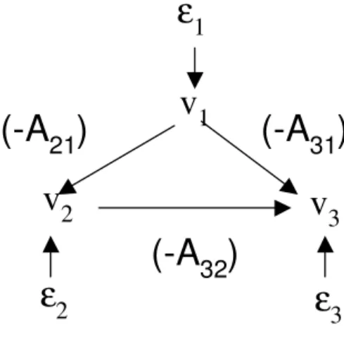
Suppose that after entering the covariance matrix of the reduced form VAR residuals, TETRAD give us the following DAG as its final output:
Figure 1 –DAG with Explicity Represented Error Terms
v
1
ε
1
v
2
v
3
ε
2
(-A
32
)
ε
3
(-A
21
)
(-A
31
)
This DAG can be represented by the following recursive system:
v1(t) = ǫ1(t)
v2(t) = −A21v1(t) +ǫ2(t)
v3(t) = −A31v1(t)−A32v2(t) +ǫ3(t)
whereǫi(t)are error terms(i= 1,2,3).
19Two linear-normal recursive Structural Equation Models are observationally equivalent if and only if they entail the same sets
of zero partial correlations.
The corresponding matrixA0is given by
A0=
1 0 0
A21 1 0
A31 A32 1
where the necessary condition for identification is satisfied.
5.3. Caveats of the Spirtes-Glymour-Scheines Methodology
SGS have shown that under some weak conditions – the Markov Condition and Faithfulness – there exist methods for identification of causal relations that are asymptotically (in sample size) correct. The SGS claim that it is possible to make causal inferences based on associations observed in
non-experimental data without background knowledge came under fierce criticism.20
Using Bayesian methods, Robins and Wasserman (1999) showed that SGS implicitly admit that, for the set of studied variables, the probability of no unmeasured common causes is positive and not small relative to the sample size. If this is not true, then SGS analysis can lead to inappropriate causal conclusions. They claim that in studies with observational data, as those in economics and other areas, the assumption that this probability is small relative to the sample size, better reflects the position of researchers.
Robins et al. (2003) used classical methods to analyze carefully the asymptotic properties of SGS methodology. They showed that the asymptotically consistent procedures of SGS are pointwise
consis-tent, but not uniform consistent.21 Furthermore, they also showed that there exists no causality test,
based on associations of non-experimental data under the Markov and faithfulness assumptions, which is uniform consistent. Therefore, for any finite sample, it is impossible to guarantee that the results of the SGS causality tests (or any other causality test) will converge to the asymptotic results.
The difficulties of the SGS procedure can be illustrated using the recursive system of section 5.2.
In the recursive model, the parameterA21measures de direct effect of v1 onv2,A32the direct
effect ofv2 onv3andA31the direct effect ofv1onv3. In the modelv2is a direct cause ofv3if and
only ifA326= 0. In other words, in a causal graph of the model there is an arrow fromv2tov3if and
only ifA326= 0. If we know that the true causal effects are an unknown subset of the ones presented
in figure 1, the conditional independence ofv2andv3, under the other hypotheses of the model, can
be straightfully tested byH0:A32= 0againstH1:A326= 0.
Suppose we want to indirectly test, as in the SGS methodology, the conditional independence
be-tweenv2andv3through the estimated sample covariance between them. If thecov(v2, v3)is exactly
equal to zero, cov(v2, v3) = −A32+A21A31 = 0, then (considering the previous paragraph’s
as-sumption about the true causal effects) there are two possible causes for the zero correlation. One
possibility is thatA32and at leastA21 orA31 are equal to zero. In this case, inferring thatv2 does
not causev3, from the zero correlation, is correct. On the other hand, even ifA32is large we can still
obtain a zero correlation betweenv2andv3ifA32 = A21A31. However, adopting faithfulness (the
Faithfulness Condition adopted by the SGS methodology) we assume that no conditional independence relation is hidden by this unlikely combination of parameters, which have Lebesgue measure equal to
zero (is very unlikely). A distribution for whichA32 =A21A31is unlikely and unfaithful to the DAG
G, representing this model, since it shows exactly zero correlation between two variables not because of missing arrows in the DAG but because parameters exactly canceling each other in the correlation,
20See for example, Humphreys and Freedman (1996, 1999), Korb and Wallace (1997), and Robins and Wasserman (1999).
21A pointwise consistent test is guaranteed to avoid incorrect decision if the sample size can be increased indefinitely. However,
132
Brisne Céspedes, Elcyon Lima e Alexis Maka
A32 = A21A31. Under the SGS model, it is sufficient to have a samplecov(v2, v3)exactly equal to
zero to deduce thatv2is not a cause ofv3. However, if the sample correlation betweenv2andv3is not
exactly zero (as will almost always happens in finite samples) and the true model is unknown, as Robins et al. (2003) have shown, the acceptance or rejection of the null hypothesis of zero partial correlation
is not unequivocally tied to the presence of conditional independence.22 Without strong additional
as-sumptions, there are no statistical tests based on correlations to determine that the causal effect is zero. This is true because Faithfulness has implications only for cases where the partial correlation is exactly zero (a unlikely case in finite samples). It does not rule out arbitrarily small partial correlations with the
edge coefficient(A32)been arbitrarily large (not very unlikely in finite samples). Zhang (2002), Zhang
and Spirtes (2003) proposed stronger versions of the faithfulness assumption that eliminate this latter possibility. Intuitively, these stronger assumptions say that small partial correlations indicate small di-rect causal effects. They show that these strengthened versions of faithfulness if true are sufficient to render the SGS model uniformly consistent.
In this article we assume that small partial correlations indicate small direct causal effects. This strong assumption is implicitly adopted in the procedures proposed by SGS.
6. MONETARY POLICY DEVELOPMENTS SINCE THE REAL PLAN
The Real Plan introduced several changes in the rules of monetary policy to achieve inflation
sta-bilization.23 The Provisional Measure (PM) no. 566 of July 29th of 1994, which implemented these
changes, established quarterly limits for money expansion in the new currency, the real.24 Starting
in the first quarter of 1995 the procedure of setting monetary limits was substituted for a monetary programming with quarterly projections for the expansion of monetary base (restricted and extended), M1, and M4 (the broadest monetary aggregate), formulated by the Central Bank and submitted to the Congress for evaluation, after approval by the National Monetary Council (CMN).
Although the new currency (the Real) was introduced at a rate of one-to-one to the U.S. dollar, there was no official commitment to any exchange rate policy. At first the Central Bank did not intervene in
22When the sample correlation is not exactly zero, it is not possible to determine which significance level should be used to test
for zero partial correlation when attempting to test for conditional independence. The significance level cannot be interpreted as the probability of type I error for the pattern output, but merely as a parameter of the search. Based on simulation tests with random DAGs, SGS suggests setting the significance level at 20% for sample size smaller than 100; at 10% for sample size between 100 and 300; and at 0.5% (or smaller) for larger samples. We followed their suggestion and set the significance level at 20%. We tested different levels of significance in the neighborhood of the chosen level (20%) and noticed that the contemporaneous causality relationships assigned by TETRAD didn’t changed.
23As source of information this section used Lopes (2003), several issues of the Boletim do Banco Central do Brasil for the period,
the provisional measures cited in the text, Central Bank of Brazil (1999), the IMF Survey of November 16, 1998 and December 14, 1998, the Boletim Conjuntural IPEA of January 1999, as well as information contained in the homepage of the Central Bank of Brazil (www.bcb.gov.br).
24The ceilings for monetary base in the third and fourth quarters of 1994 were set at R$ 7,5 billion and R$ 8,5 billion, respectively.
However, the same PM allowed the National Monetary Council (CMN) to authorize an extra margin of up to 20% of these limits. Neither the PM no. 566 nor the PM no. 596 (its update), defined how the monetary ceilings should be measured. This was set as responsibility of the CMN, who later chose the daily average balance concept. In the July-September quarter the monetary base - measured by average daily balances – reached R$ 8.9 billion, slightly below the R$ 9 billion ceiling once the 20% extra margin was approved by the CMN on August 24th [the monetary base measured by end of period balances reached R$ 12,8 billion at the end of the third quarter of 1994]. The monetary limit for the last quarter of 1994 was reviewed twice. The PM no. 681 of October 27th of 1994 substituted the original limit of R$ 8,5 billion substituted by a new limit that allowed an increase of 13.33% over the balances observed at the end of September, meaning that the new limit was R$ 14,5 billion. Then, on December 21st the CMN approved a new ceiling of R$ 15,1 billion. The average daily balance of the monetary base of the October-December quarter reached R$ 14,8 billion. The Provisional Measure no. 681 also introduced the concept of extended monetary base together with the establishment of a zero growth rate for it during the last quarter of 1994 (the extended base adds federal government securities in the market (except LBC-E) to the traditional concept of monetary base). The CMN authorized on December 21st a growth rate of 3.5% for the extended base, whose effective growth reached 1.9%.
the foreign currency market and the Real appreciated vis-à-vis the dollar. The Central Bank reports that
it began intervening in the exchange rate market in the second half of September.25 On March 10th
of 1995 the Central Bank introduced a formal 0.88-0.93 exchange rate band with the commitment to intervene only on its limits, after an unsuccessful attempt to introduce a narrower band a day before when it lost 4 billion dollars in international reserves (see Figure 2). At the same time the SELIC interest rate was sharply increased in order to prevent any speculation against the Real (see Figure 3).
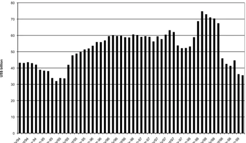
Figure 2 –International Reserves, from July 94 to February 1999 (note: the amounts pictured above include US$ 9.3 billion received on December 1998 as part of the financial program coordinated by the IMF)
0 10 20 30 40 50 60 70 80
july/ 94
sept
/94
Nov-9
4
Jan-9
5
Mar-9
5
ma
y/95
july/ 95
sept
/95
Nov-9
5
Jan-9
6
Mar-9
6
ma
y/96
july/ 96
sept
/96
Nov-9
6
Jan-9
7
Mar-9
7
ma
y/97
july/ 97
sept
/97
Nov-9
7
Jan-9
8
Mar-9
8
ma
y/98
july/ 98
sept
/98
Nov-9
8
Jan-9
9
U
S$
b
il
li
o
n
On June of 1995 a new 0.91-0.99 exchange rate band was announced together with the introduction of a new mechanism of intervention in the foreign exchange market, the “spread-auction”, that in
practice resulted in an exchange rate peg (see figure 4) through what became know as “mini-bands”.26
There was no official rule for the speed of the crawling but it was understood that it was being set so as to slowly devaluate the Real.
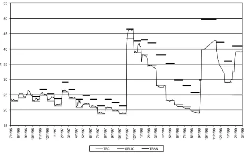
On June 20th of 1996 the Monetary Policy Committee (COPOM) was created with the objective of setting the stance of monetary policy and the short-term interest rate. The design of monetary policy operational procedure was modified with the introduction of two new interest rates – the TBC and the
TBAN.27According to Lopes (2003), in this setup inspired in the Deutsche Bundesbank the TBC, the rate
at which banks could have financial assistance through rediscount window of the Central Bank, played the role of an interest rate floor, and the TBAN the ceiling. In principle, the SELIC rate would be allowed to fluctuate freely inside this interest rate band, with the values of both TBC and TBAN rates being determined by the COPOM. However, in practice the Central Bank managed to put the SELIC rate close to the TBC rate most of the time (see figure 5).
25See the Boletim do Banco Central do Brasil of November 1994.
26Notice that the “mini-bands” are not pictured in figure 5, only the “regular” bands.
134
Brisne Céspedes, Elcyon Lima e Alex is Maka Figur e 3 – SELIC Overnight Inter est Rate, Ann ualized 15 25 35 45 55 65 75 85
8/1/94 10/1/94 12/1/94 2/1/95 4/1/95 6/1/95 8/1/95 10/1/95 12/1/95 2/1/96 4/1/96 6/1/96 8/1/96 10/1/96 12/1/96 2/1/97 4/1/97 6/1/97 8/1/97 10/1/97 12/1/97 2/1/98 4/1/98 6/1/98 8/1/98 10/1/98 12/1/98 2/1/99 % SEL IC O v e rn ig h t In te re s t R a te , A n n u a lize d Figur e 4 – Ex change Rate (R$/US$), fr om July 199 4 to Januar y 1999
0.8 0.85 0.9 0.95
1
1.05 1.1 1.15 1.2 1.25
01/07/94 01/09/94 01/11/94 01/01/95 01/03/95 01/05/95 01/07/95 01/09/95 01/11/95 01/01/96 01/03/96 01/05/96 01/07/96 01/09/96 01/11/96 01/01/97 01/03/97 01/05/97 01/07/97 01/09/97 01/11/97 01/01/98 01/03/98 01/05/98 01/07/98 01/09/98 01/11/98 01/01/99 Exchange Rate
Band Lower Limit
Band Upper Limit
Figure 5 –Overnight Interest Rates, Annualized - from July 1996 to March 1999 15 20 25 30 35 40 45 50 55 7 /1 /9 6 8 /1 /9 6 9 /1 /9 6 1 0 /1 /9 6 1 1 /1 /9 6 1 2 /1 /9 6 1 /1 /9 7 2 /1 /9 7 3 /1 /9 7 4 /1 /9 7 5 /1 /9 7 6 /1 /9 7 7 /1 /9 7 8 /1 /9 7 9 /1 /9 7 1 0 /1 /9 7 1 1 /1 /9 7 1 2 /1 /9 7 1 /1 /9 8 2 /1 /9 8 3 /1 /9 8 4 /1 /9 8 5 /1 /9 8 6 /1 /9 8 7 /1 /9 8 8 /1 /9 8 9 /1 /9 8 1 0 /1 /9 8 1 1 /1 /9 8 1 2 /1 /9 8 1 /1 /9 9 2 /1 /9 9 3 /1 /9 9 %
TBC SELIC TBAN
Note: the TBC rediscount window was closed from September 4th of 1998 to December 16th of 1998.
The Asian Crisis28 and the Russian default29 affected Brazil through the loss of international
re-serves, which caused sharp interest rate increases on October 1997 and September 1998. The monetary policy during these periods was dominated by the Brazilian government attempt to defend the real. On September 4th, 1998 there was a change in the operational procedure of the Central Bank: the redis-count window at the TBC rate was closed, making the SELIC rate jump to the TBAN rate. Despite the government’s efforts, the international reserves kept sliding. On November 13th, 1998 Brazil and the International Monetary Fund (IMF) announced the conclusion of negotiations on a financial program that provided support of U$ 41.5 billion over the next three years, making U$ 37 billion available, if needed, over the next 12 months. The Central Bank gave up defending the exchange rate on January 15th, 1999 and announced the free-floating as the new exchange rate regime on January 18th, 1999.
On March 4th of 1999 both TBC and TBAN rates were extinguished and a new monetary policy op-erational procedure was introduced. In this new framework the COPOM sets a target for the SELIC rate that remains constant until the next regular COPOM meetings. However, the COPOM could establish a monetary policy bias at its regular meetings; a bias (to ease or tighten) authorizes the Central Bank’s Governor to alter the SELIC interest rate target in the direction of the bias anytime between regular
28In the wake of the Asian Crisis Brazil lost near 15% of its foreign reserves on October 28th of 1997 (see figure 3). In response,
the Central Bank increased sharply interest rates with the SELIC overnight rate reaching more than 45% per annum (it was near 20% before, see figure 6) and started to operate in the dollar futures market in order to defend the exchange rate. Despite the negative effect of the interest rate hike over the public debt, it induced a huge increase in international reserves, which moved from US$ 52 billion in November 1997 to near US$ 75 billion in April 1998 (see figure 3).
29On August 17th of 1998, the rouble devaluation and the Russian default provoked an international financial crisis. According
to Lopes, the Central Bank responded increasing interest rates in four stages (see figure 6). First, on September 2nd, the TBAN
136
Brisne Céspedes, Elcyon Lima e Alexis Maka
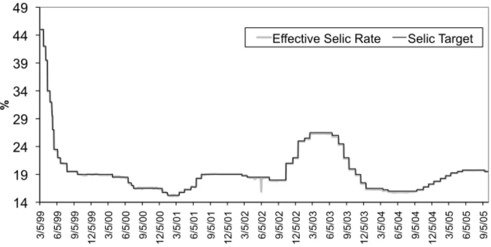
COPOM meetings. As can be seen in figure 6, in this new monetary policy framework the SELIC rate hits its target value as the Central Bank offsets total reserve demand and borrowing demand
distur-bances.30 Brazil implemented a formal inflation targeting framework for monetary policy on June 21
of 1999. Under the inflation targeting regime, the COPOM’s monetary policy decisions have as their main objective the achievement of the inflation targets set by the National Monetary Council (CMN). If inflation breaches the target set by the CMN, the Governor of the Central Bank is required to write an open letter to the Minister of Finance explaining the reasons why the target was missed, as well as the measures required to bring inflation back to the target, and the time period over which these measures are expected to take effect. The introduction of inflation targeting didn’t change the monetary policy operational procedure, which continued to be based on the control of the SELIC rate (see Figure 6).
Figure 6 –Comparison between the Target for the SELIC Rate Determined by the Central Bank and the Effective SELIC Rate
14 19 24 29 34 39 44 49 3 /5 /9 9 6 /5 /9 9 9 /5 /9 9 1 2 /5 /9 9 3 /5 /0 0 6 /5 /0 0 9 /5 /0 0 1 2 /5 /0 0 3 /5 /0 1 6 /5 /0 1 9 /5 /0 1 1 2 /5 /0 1 3 /5 /0 2 6 /5 /0 2 9 /5 /0 2 1 2 /5 /0 2 3 /5 /0 3 6 /5 /0 3 9 /5 /0 3 1 2 /5 /0 3 3 /5 /0 4 6 /5 /0 4 9 /5 /0 4 1 2 /5 /0 4 3 /5 /0 5 6 /5 /0 5 9 /5 /0 5 %
Effective Selic Rate Selic Target
As seen above, Brazil experienced several changes in policy regime in the period after the Real Plan. Therefore, in order to appropriately conduct an empirical analysis of this period it is important to divide it in subsamples sharing common features. Unfortunately, some of these subsamples are too short to allow for any type of econometric analysis. Based on the exchange rate regime and monetary policy operational procedures, we decided to partition our sample into two subsamples. The first one goes from 1996:07 to 1998:08, the period with exchange rate “mini-bands” combined with the adoption of the TBC rate as an informal target for the SELIC rate. The second one goes from 1999:03 to 2004:12, the period with free-floating exchange rate and explicit SELIC targeting.
7. BASIC MODEL AND RESULTS FOR THE FIRST SUBSAMPLE (1996:07-1998:08)
The variables selected for the Basic Model of the first subsample (BM1) are: SELIC, international reserves, price level, money (M1), output, a constant, and seasonal dummies. Given the small sample
30During the second and third quarters of 2002 the Central Bank had difficulties in hitting its SELIC target because of the decline in
the demand for public securities due to the migration of resources out of Financial Investment Funds (FIF) into other modalities of financial investment caused by the requirement of the marking-to-market methodology in pricing fund assets.
size, we restricted the analysis to lag length one, which is also the lag order selected by the Schwarz Information Criterion (SIC).
7.1. Contemporaneous Causal Ordering
Applying TETRAD at the 20% significance level31 and assuming that the variables selected for the
model are causally sufficient32, we obtain what is known as apattern,33shown in Figure 7. The pattern
is a graphical representation of the set of observationally equivalent DAGs containing the contempora-neous causal ordering of the variables. According to Figure 7 the BM1 has four observationally equiva-lent DAGs, displayed on figure 8. Each of these DAGs is a valid representation of the contemporaneous causal ordering of the BM1 according to TETRAD. In what follows we will restrict our attention to the causal ordering displayed on figure 8(b), but we would like to stress that the results discussed next do not change much when the alternative causal orderings are used. According to figure 8(b), neither the SELIC rate nor the stock of money (M1) are contemporaneously affected by the other variables of the model, with international reserves responding to changes in the SELIC rate within the same period,
suggesting the level of reserves is sensible to interest rate differentials.34 In addition, changes in output
have immediate effect on prices35
Figure 7 –Pattern of the BM1
RESERVES SELIC
M1 OUTPUT
IPCA
7.2. Impulse Response Analysis
Using the contemporaneous causal ordering of figure 8(b) to identify the BM1, we compute and ana-lyze in this section the impulse response functions of economic variables to exogenous and independent shocks.36
31See Footnote 22.
32A set of variables V is said to be causally sufficient if every common cause of any two or more variables in V is in V. TETRAD has
a bias towards excluding causal relations present in the data. To overcome this problem, SGS suggests that a 20% significance level should be used.
33A pattern is a partially oriented DAG, where the directed edges represent arrows that are common to every member in the
equivalent class, while the undirected edges are directed one way in some DAGs and another way in others. Undirected edges (—) mean that there is causality in one of the two directions but not on both, while double oriented edges (↔) mean causality on both directions.
34Notice that this result stands against the assumption made by Fernandes and Toro (2005) that international reserves are an
exogenous variable.
35We estimated an alternative model with the same variables of the BM1 using a different subsample that starts at 1995:05 and
ends at 1998:12. We noticed that TETRAD’s identification of the contemporaneous causal ordering showed some sensibility to whether the IMF loan of US$ 9.3 billion given to Brazil on December of 1998 was included or not. The exclusion of the loan led to the exclusion also of the edge between SELIC and reserves in the respective pattern.
36We will not present and discuss the parameters estimates of the model because of the difficulties associated with their
138
Brisne Céspedes, Elcyon Lima e Alexis Maka
Figure 8 –Observationally Equivalent DAGs from the Pattern of the BM1
RESERVES SELIC
M1 OUTPUT
IPCA
Figure 8 (a)
RESERVES SELIC
M1 OUTPUT
IPCA
Figure 8 (b)
RESERVES SELIC
M1 OUTPUT
IPCA
Figure 8 (c)
RESERVES SELIC
M1 OUTPUT
IPCA
Figure 8 (d)
The impulse response functions (IRFs) displayed on figure 937show that output and money fall in
response to a positive SELIC shock.38 The large uncertainty of the response of the price level to a SELIC
shock (reflected in large probability bands) is not surprising, due to the small sample size, and indicates that we should be cautious when inferring what is the response of the price level to a SELIC shock. However, the most likely result (indicated by the solid line between the bands) is that the price level
goes down in response to a SELIC innovation.39 Positive money shocks on the other side have a more
immediate effect over prices but no significant effect on the SELIC rate. Positive international reserves shocks decrease interest rates and stimulate economic activity, leading to an increase in inflation. The results for this period suggest that SELIC shocks are the best candidates for representing monetary policy shocks.
8. BASIC MODEL AND RESULTS FOR THE SECOND SUBSAMPLE (1999:03-2004:12)
The variables selected for Basic Model of the second subsample (BM2) are not all the same as those chosen for the Basic Model of the first subperiod (BM1). The differences are that we substituted the exchange rate for the international reserves, given that now there is free floating of the exchange rate, and substituted the medium term interest rate (SWAP) for money because the Central Bank started targeting (explicitly) the short-run interest rate. Therefore, the BM2 is composed by: SELIC, exchange rate, price level, SWAP, output, a constant, and seasonal dummies. The chosen lag length of the BM2 is one, following the Schwarz information criterion (SIC).
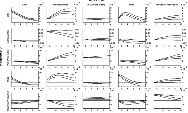
8.1. Contemporaneous Causal Ordering
Using TETRAD to find out the contemporaneous causal ordering of the BM2,40we obtain the pattern
displayed on figure 10, containing just one DAG, used to identify the BM2.
According to the identification suggested by TETRAD, SELIC shocks affect output and the SWAP rate contemporaneously. This result is a departure from the widely used identification assumption that the variables in the Central Bank information set do not respond to monetary policy shocks within the
37The error bands for impulse responses were constructed following the methodology suggested bySims and Zha (1999).
38By “positive” SELIC shock we mean an unexpected increase in the SELIC rate. This type of shock is also referred in the literature
as “contractionary” because it is supposed to contract economic activity.
39In an alternative model for the 1995:05-1998:12 subperiod, where the exchange rate and the SWAP rate were used instead of
international reserves and M1, we observed an increase in the price level in response to a SELIC shock, without taking into account the uncertainty of the period.
40See footnote 22.
Figure 9 –Observationally Equivalent DAGs from the Pattern of the BM1
Selic
2 4 6 8 10
-0.01 0 0.01 0.02 0.03 Selic
2 4 6 8 10
-0.01 0 0.01 0.02 0.03 Reserves
2 4 6 8 10
-0.01 0 0.01 0.02 0.03 IPCA (Price Index)
2 4 6 8 10
-0.01 0 0.01 0.02 0.03 M1
2 4 6 8 10
-0.01 0 0.01 0.02 0.03 Industrial Production Reserves
2 4 6 8 10
-0.02 0 0.02 0.04 0.06
2 4 6 8 10
-0.02 0 0.02 0.04 0.06
2 4 6 8 10
-0.02 0 0.02 0.04 0.06
2 4 6 8 10
-0.02 0 0.02 0.04 0.06
2 4 6 8 10
-0.02 0 0.02 0.04 0.06
IPCA (Price Index)
2 4 6 8 10
-4 -2 0 2
x 10-3
2 4 6 8 10
-4 -2 0 2
x 10-3
2 4 6 8 10
-4 -2 0 2
x 10-3
2 4 6 8 10
-4 -2 0 2
x 10-3
2 4 6 8 10
-4 -2 0 2
x 10-3
M1
2 4 6 8 10-0.1
-0.05 0
2 4 6 8 10-0.1
-0.05 0
2 4 6 8 10-0.1
-0.05 0
2 4 6 8 10-0.1
-0.05 0
2 4 6 8 10-0.1
-0.05 0
Industrial Production
2 4 6 8 10
-20 -10 0
x 10-3
2 4 6 8 10
-20 -10 0
x 10-3
2 4 6 8 10
-20 -10 0
x 10-3
2 4 6 8 10
-20 -10 0
x 10-3
2 4 6 8 10
-20 -10 0
x 10-3
Response of
Shock to
Figure 10 –Pattern of the BM2
EXCHANGE RATE SELIC
SWAP OUTPUT
IPCA
current period.41 Additionally, we observe that in TETRAD’s identification, none of the variables affect
contemporaneously the SELIC rate, even the price level and the output. The fact that output and prices have no contemporaneous effect over the SELIC rate may be associated with the difficulty of obtaining information on the current level of output and price level by the time policy makers have to make their decisions, an assumption made, for example, by Sims and Zha (2006).
41Christiano et al. (1999) refer to this assumption as the recursiveness assumption. It implies that economic variables within the
140
Brisne Céspedes, Elcyon Lima e Alexis Maka
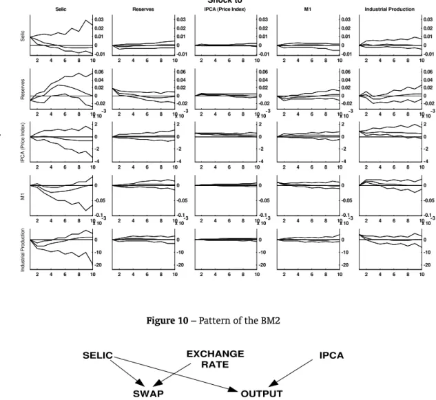
8.2. Impulse Response Analysis and Variance Decomposition
Using the contemporaneous causal ordering of figure 10 to identify the BM2 we obtained the IRFs displayed on Figure 11.
Figure 11 –IRFs of the Benchmark Model 1999:03 - 2004:12, with 68% Probability Bands (lag = 1)
Selic
2 4 6 8 10
-2 0 2 4 6 8 x 10 -3 Selic
2 4 6 8 10
-2 0 2 4 6 8 x 10 -3 Exchange Rate
2 4 6 8 10
-2 0 2 4 6 8 x 10 -3 IPCA (Price Index)
2 4 6 8 10
-2 0 2 4 6 8 x 10 -3 Swap
2 4 6 8 10
-2 0 2 4 6 8 x 10 -3 Industrial Production Exchange Rate
2 4 6 8 10
-0.02 0 0.02 0.04 0.06
2 4 6 8 10
-0.02 0 0.02 0.04 0.06
2 4 6 8 10
-0.02 0 0.02 0.04 0.06
2 4 6 8 10
-0.02 0 0.02 0.04 0.06
2 4 6 8 10
-0.02 0 0.02 0.04 0.06
IPCA (Price Index)
Response of
2 4 6 8 10
0 5 10 x 10
-3
2 4 6 8 10
0 5 10 x 10
-3
2 4 6 8 10
0 5 10 x 10 -3
2 4 6 8 10
0 5 10 x 10
-3
2 4 6 8 10
0 5 10 x 10 -3 Swap
2 4 6 8 10
0 5 10
x 10-3
2 4 6 8 10
0 5 10
x 10-3
2 4 6 8 10
0 5 10
x 10-3
2 4 6 8 10
0 5 10
x 10-3
2 4 6 8 10
0 5 10
x 10-3
Industrial Production 2 4 6 8 10 -5 0 5 x 10
-3
2 4 6 8 10
-5 0 5 x 10
-3
2 4 6 8 10
-5 0 5 x 10
-3
2 4 6 8 10
-5 0 5 x 10
-3
2 4 6 8 10
-5 0 5 x 10 -3 Shock to
As can be seen in Figure 11, the responses to a positive SELIC innovation are in line with the results that one would expect from (contractionary) monetary policy shocks: the exchange rate appreciates, output decreases, and the price level goes down. It is interesting to note the lag with which the price level responds to a (positive) SELIC shock: it takes near six months until the price level starts to fall despite the immediate and persistent contraction of economic activity, that returns to its pre-shock level after one year.
Using the same structural decomposition of the IRFs to calculate the variance decomposition, we observe that a substantial portion of the forecast error variance of the SELIC rate can be attributed to exchange rate shocks, about 61% after twelve months, with Swap shocks responding to 13%, while output and price level shocks represent 3-5% and 0.02%, respectively (see Table 1).
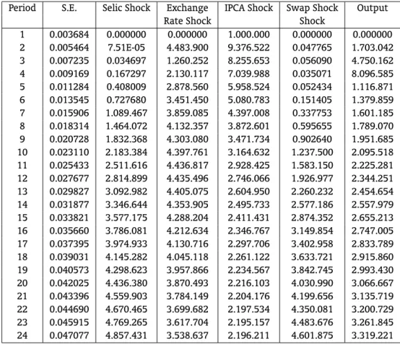
Unexpected exchange rate devaluations are inflationary with the price level starting to increase one month after the exchange rate shock hits the economy. In fact, exogenous shocks to the exchange rate are for the 1999-2004 period, the most important exogenous source of inflation rate fluctuation, as can be seen more clearly in the variance decomposition of the price level, displayed on table 2. With 12 months ahead, the exchange rate shock is responsible for near 45% of forecast error variance of the price level. Despite the persistence of the (positive) exchange rate shock, the resulting increase in inflation and in interest rates imply that there is a contraction in the level of economic activity.
The increase in the price level in response to positive output shocks suggests that they are associ-ated with demand shocks. This inflationary effect explains why interest rates goes up in response to (positive) output shocks in the second subsample.
Table 1 –Variance Decomposition of SELIC
Period S.E. Selic Shock Exchange IPCA Shock Swap Shock Output
Rate Shock Shock
1 0.006504 1.000.000 0.000000 0.000000 0.000000 0.000000
2 0.009226 8.419.765 1.090.360 0.000215 1.447.120 0.240568
3 0.011275 6.908.451 5.918.915 0.003608 2.471.916 0.273804
4 0.012908 5.695.910 1.470.535 0.011013 2.811.397 0.210569
5 0.014352 4.716.222 2.560.766 0.019887 2.697.736 0.232886
6 0.015724 3.942.947 3.621.287 0.027274 2.390.226 0.428127
7 0.017036 3.359.299 4.494.470 0.031778 2.064.566 0.784878
8 0.018252 2.935.975 5.136.890 0.033568 1.799.126 1.246.526
9 0.019331 2.636.984 5.574.450 0.033499 1.609.633 1.755.829
10 0.020249 2.429.200 5.855.154 0.032450 1.485.295 2.271.059
11 0.021000 2.286.453 6.024.696 0.031064 1.409.177 2.765.680
12 0.021592 2.189.538 6.118.989 0.029723 1.366.126 3.223.747
13 0.022043 2.124.776 6.164.110 0.028611 1.344.654 3.635.988
14 0.022376 2.082.473 6.178.363 0.027778 1.336.646 3.997.398
15 0.022613 2.055.719 6.174.399 0.027198 1.336.564 4.305.972
16 0.022776 2.039.546 6.160.856 0.026815 1.340.710 4.562.058
17 0.022884 2.030.362 6.143.518 0.026567 1.346.668 4.767.955
18 0.022953 2.025.575 6.126.118 0.026408 1.352.908 4.927.580
19 0.022995 2.023.344 6.110.892 0.026317 1.358.524 5.046.090
20 0.023021 2.022.393 6.098.994 0.026300 1.363.036 5.129.468
21 0.023036 2.021.884 6.090.808 0.026387 1.366.262 5.184.077
22 0.023047 2.021.303 6.086.195 0.026626 1.368.215 5.216.248
23 0.023056 2.020.377 6.084.693 0.027075 1.369.030 5.231.920
24 0.023065 2.019.005 6.085.674 0.027796 1.368.905 5.236.377
8.3. Robustness of the Basic Analysis
In this section we analyze the robustness of the results of the Basic Model of the second subperiod (BM2) to two changes in the original model. First, we consider the effects of different lag lengths of the VAR model. Second, we analyze the consequences of introducing money in the basic model.
8.3.1. Different Lag Lengths
We estimated alternative models using the same variables of the basic model employing different
lag lengths.42 Figures 12 and 13 show the contemporaneous causal orderings provided by TETRAD for
lag lengths 2 and 3, respectively, used to identify the IRFs.43 Notice that TETRAD provides different
orderings for each lag length as a result of differences in the estimated covariance matrices. Despite the differences in identification, the qualitative features of these IRFs, displayed on Figures 14 and 15, aren’t much different from those of the BM2 (Figure 11), with the exception the response of the price level to monetary policy shocks. For lags 2 and 3 the price level temporarily increases in response to a
42Starting with lag length three, the residuals exhibit no autocorrelation. For this reason, here we restrict our analysis to lag
lengths up to three.
43Undirected edges (—) mean that there is causality in one of the two directions but not on both. In what follows we will
142
Brisne Céspedes, Elcyon Lima e Alexis Maka
Table 2 –Variance Decomposition of SELIC
Period S.E. Selic Shock Exchange IPCA Shock Swap Shock Output
Rate Shock Shock
1 0.003684 0.000000 0.000000 1.000.000 0.000000 0.000000
2 0.005464 7.51E-05 4.483.900 9.376.522 0.047765 1.703.042
3 0.007235 0.034697 1.260.252 8.255.653 0.056090 4.750.162
4 0.009169 0.167297 2.130.117 7.039.988 0.035071 8.096.585
5 0.011284 0.408009 2.878.560 5.958.524 0.052434 1.116.871
6 0.013545 0.727680 3.451.450 5.080.783 0.151405 1.379.859
7 0.015906 1.089.467 3.859.085 4.397.008 0.337753 1.601.185
8 0.018314 1.464.072 4.132.357 3.872.601 0.595655 1.789.070
9 0.020728 1.832.368 4.303.080 3.471.734 0.902640 1.951.685
10 0.023110 2.183.384 4.397.761 3.164.632 1.237.500 2.095.518
11 0.025433 2.511.616 4.436.817 2.928.425 1.583.150 2.225.281
12 0.027677 2.814.899 4.435.496 2.746.066 1.926.977 2.344.251
13 0.029827 3.092.982 4.405.075 2.604.950 2.260.232 2.454.654
14 0.031877 3.346.644 4.353.905 2.495.733 2.577.186 2.557.979
15 0.033821 3.577.175 4.288.204 2.411.431 2.874.352 2.655.213
16 0.035660 3.786.081 4.212.634 2.346.767 3.149.854 2.747.005
17 0.037395 3.974.933 4.130.716 2.297.706 3.402.958 2.833.789
18 0.039031 4.145.282 4.045.118 2.261.122 3.633.721 2.915.860
19 0.040573 4.298.623 3.957.866 2.234.567 3.842.745 2.993.430
20 0.042025 4.436.380 3.870.493 2.216.103 4.030.990 3.066.667
21 0.043396 4.559.903 3.784.149 2.204.176 4.199.656 3.135.719
22 0.044690 4.670.465 3.699.682 2.197.534 4.350.081 3.200.729
23 0.045915 4.769.265 3.617.704 2.195.157 4.483.676 3.261.845
24 0.047077 4.857.431 3.538.637 2.196.211 4.601.875 3.319.221
positive SELIC shock, a result known in the literature as the “price puzzle”, since it is at odds with most theoretical models’ prediction that restrictive monetary policy should reduce the price level.
Figure 12 –Pattern of the Benchmark Model with Lag Length 2
EXCHANGE RATE SELIC
SWAP OUTPUT
IPCA
143
Figure 13 –Pattern of the Benchmark Model with Lag Length 3
EXCHANGE RATE SELIC
SWAP OUTPUT
IPCA
Observationally equivalent DAGs from the pattern of the figure 13
EXCHANGE RATE SELIC
SWAP OUTPUT
IPCA
Figure 13 (a)
EXCHANGE RATE SELIC
SWAP OUTPUT
IPCA
Figure 13 (b)