A Case for Cross Layer Design: The Impact
of Physical Layer Properties on Routing
Protocol Performance in MANETs
Lecturer Mangesh D. Nikose
Department of Electrical Engineering, VJTI, Matunga, Mumbai, India.
Anni U. Gupta
Lecturer Department of E&Tc Engineering,MET’s BKC IOE, Nashik, India
Abstract−
In this paper, we evaluate the performance of routing protocols for mobile ad hoc network using different physical layer models. The results obtained shows that the performance obtained using idealized models such as the free space propagation model vary significantly when propagation effects, as path loss and shadowing are considered. This difference in performance indicates that optimization is required in the protocol development space that takes into account channel state information (CSI). Such an optimization requires a cross layer design approach to be adopted and a framework for protocol performance evaluation to be established. This work would serve as a first step in this direction and here we provide comparative performance results through network simulations.
Keywords− Ad hoc networks; Cross layer Design; Routing.
1. Introduction
Mobile Ad hoc Networks (MANETs) are self-organizing and self-configuring multi-hop wireless networks capable of adaptive re-configuration as effected by node mobility. Typically the network is made up of equal nodes that are equipped for wireless communication and with networking capability. Every node in the network is capable of functioning as a mobile router (i.e., maintain routes & forward packets), this makes possible the multi-hop forwarding of packets from a source node to a destination node without reliance on a fixed infrastructure. All nodes share the same random access wireless channel. With almost all development in information technology being based on wireless technology, ad hoc networks are expected to play a significant role in future communication networks where wireless access to a backbone is either ineffective or impossible.
Routing in MANETs has received significant attention in the research community over the past few years. This has seen the development of several routing protocols. Proactive as well as on-demand routing schemes have been proposed in literature [1]. The performance evaluation of these protocols has invariably focused on the impact of node mobility on the performance of these protocols. The mobility models used have been varied ranging from individual to group mobility models. Further, each of these performance evaluations has assumed a free space propagation model ignoring the time varying aspects of the wireless channel and its properties such as path loss, multipath fading and shadowing. This is reflected in the assumption a fixed transmission range for each node in the network. In a real world deployment a fixed transmission range is not achievable. As a result the performance of these protocols are less than optimal and do not guarantee the same level of performance in real world deployments.
Next generation networks (3G & beyond) are envisioned to support real time services making use of WLAN, hot spot and ad hoc network technologies. A real-time flow is required to deliver data packets with strict timing requirements. Hence, there is a requirement for optimized routing protocol performance. However, achieving quality of service (QoS) requirements will be impossible if route construction and maintenance procedures do not take into account the time varying characteristics of the wireless channel (such as channel capacity). This optimization can also be extended to other spheres such as co-operative diversity [2] that can benefit application performance in an opportunistic manner. This is only possible if a cross layer approach is adopted. Cross layer design is best defined as a departure from the reference architecture model that does not allow direct communication between non-adjacent layers or the sharing of variables (e.g., TCP/IP or OSI) [3].
models that take into account of two main characteristics of the wireless channel as path loss and shadowing. Also the performances of protocols in this setting and in idealized free space propagation setting are compared through network simulations. Section II describes an overview of ad hoc routing protocols. The propagation models used in our simulations is present in Section III. Finally, section IV and section V are about simulation study and conclusions of our work.
2. Routing In MANETS
Routing in ad hoc networks faces extreme challenges from node mobility/dynamics, potentially very large number of nodes and limited communication resources (e.g., bandwidth and energy) [1]. This has prompted significant research in this domain. In this section we present a high level view of six routing protocols. The reader is directed to the specific literature for a more in depth treatment.
Ad Hoc On Demand Distance Vector (AODV)
AODV [4] is classified as a pure on-demand route acquisition system since nodes that are not on a selected path do not maintain any routing information or participate in routing table exchanges. AODV typically reduces the number of required updates by creating routes on-demand as opposed to maintaining a complete list of routes to all destinations. In AODV when a route to a destination is required and a valid route is not available, a route discovery process is initiated. The source broadcasts its request to its neighbors who in turn forward it to their neighbors and so on. To reduce the route discovery overhead the request is dropped if an intermediate node that receives the request has a valid route to the destination. If not the request propagates until the destination is reached.
AODV employs backward learning (i.e., on receiving a request the transit nodes learn the path to the source), which enables the destination to send the route request reply along the path taken by the query. The intermediate nodes that receive the route reply set up active forward routes in their routing tables that point to the node that generated the route reply. This path of active forward routes becomes the route that is employed. Once a route has been chosen it is maintained as long as it is in use by the source. A link-failure or topology change is reported recursively through all intermediate nodes to the source, which triggers another route discovery process to identify an alternate route.
Dynamic Source Routing (DSR)
DSR [5] is on-demand routing protocol that is source-initiated. The sender explicitly lists the route in the packet’s header, identifying each forwarding “hop” by the address of the next node to which to transmit the packet on its way to the destination host. The DSR protocol consists of two mechanisms: Route Discovery and Route Maintenance.
In DSR each node receiving a route request checks its cache to see if it possesses a valid route to the destination. If not it adds its own address to the route record of the request packet before forwarding. A route reply message is initiated in response to a route request by either the destination node or an intermediate node that has a valid route to the destination. In the route reply message the destination node provides the source with the route record from its corresponding route request. The route reply message can be returned either by source routing from the destination node back to the source node or by route reversal in the case of symmetric links being used. Otherwise a route discovery process for the route reply message is to be initiated. In the event of link failure, route reconstruction can be delayed if the source has an alternate route to the destination. If not route discovery would need to be initiated. The overhead of the route discovery process increases linearly with the number of nodes in the network.
Location Aided Routing (LAR)
belong to the request zone. If a path cannot be found within a predefined time period then the entire network space is included in the following route request. The probability of finding a path increases as the request area increases. However the route discovery overhead also increases with the size of the request zone. In LAR scheme1, the request zone is defined as the smallest rectangle that contains the current location of the source and the expected zone of the destination such that the sides of the rectangle are parallel to the co-ordinate axes. The source node determines the four corners of the rectangle and includes their coordinates in the route request message. Receiving node is thus able to determine if it is in the request zone and forwards or discards the route request accordingly.
Landmark Adhoc Routing Protocol (LANMAR)
LANMAR [7] has been proposed for large scale ad hoc networks that exhibit group mobility characteristics. If there exists a commonality of interest then the nodes of the ad hoc network will move as a group (e.g., battalions in military situations). In that case it is possible to identify logical subnets. Each logical subnet elects one of its nodes to act as a landmark and these are used to keep track of each subnet. Routing information regarding all landmarks is propagated by a distance vector scheme such as DSDV [8]. LANMAR also incorporates a local scope routing scheme for routing within a given scope D for a node. Each node has detailed topology information about nodes within its local scope and a distance and routing vector to all landmarks. When the destination is within the local scope then the RIP [9] routing tables are used. If the destination is outside the scope then the packet is routed to the destination landmark. Once the packet arrives within the scope of the destination then routing using the RPI routing information is resumed. LANMAR employs an IP like address consisting of group-ID (subnet ID) and a host ID <Grouped, Hosted> to identify each node. LANMAR reduces both routing table size and control overhead effectively through the localized routing table and grouped routing table for remote destinations.
Routing Information Protocol (RIP)
The Routing Information Protocol, or RIP, as it is more commonly called, is one of the most enduring of all routing protocols Routing Information Protocol is an Interior Gateway Protocol used to exchange routing information within a domain or autonomous system. RIP lets routers exchange information about destinations for the purpose of computing routes throughout the network. Destinations may be individual hosts, networks, or special destinations used to convey a default route. RIP is based on the Bellman-Ford or the distance-vector algorithm. This means RIP makes routing decisions based on the hop count between a router and a destination. RIP does not alter IP packets; it routes them based on destination address only. The maximum number of hops in a path is 15 RIP uses numerous timers to regulate its performance. These include a routing-update timer, a route-timeout timer and a route-flush timer. The routing-update timer clocks the interval between periodic routing updates. Generally, it is set to 30 seconds, with a small random amount of time added whenever the timer is reset. The IP address of the sender is used as the next hop.
Despite RIP's age and the emergence of more sophisticated routing protocols, it is far from obsolete. RIP is mature, stable, widely supported, and easy to configure. Its simplicity is well suited for use in stub networks and in small autonomous systems that do not have enough redundant paths to warrant the overheads of a more sophisticated protocol.
Zone Routing Protocol (ZRP)
3. Path Loss And Shadowing
The aim of a propagation model is to predict the received signal power of each packet. The received signal power impacts on the ability of the receiver to decode the received packet and is dependent on the path loss that is experienced also other effects of the wireless channel such as shadowing and fading. For an accurate estimate of the path loss that is experienced by various models including empirical models have been proposed. Here we present the two path loss models that are used in our simulations. Further we describe two shadowing models that are used as lognormal shadowing and constant shadowing. Free space propagation models assume zero shadowing.
Free Space Propagation
The free space model [11] represents the communication range as an imaginary circle around the transmitter. If a receiver is within the circle, it receives all packets; otherwise it loses all packets. This model is mostly used when a MANET is employed in an open-field like environment.
The free space propagation model assumes the ideal propagation condition, where there is only one clear line-of sight path between the transmitter and the receiver. The transmission loss is due to the propagation distance only. Giving a distance d between the transmitter and the receiver, the received signal power Pr(d) is given according to Fries free-space equation as,
Pt. Gt. Gr. 2
Pr(d) = (1) (4 . d)2 .L
Where Pt is the transmitted signal power, Gt and Gr are the antenna power gain of the transmitter and receiver respectively, a constant L is the system loss and is the wavelength. So, the path loss is
(2)
Two Ray Ground Reflection
The two-ray ground reflection model [11] considers both the direct path and a ground reflection path, when a single line of sight path between two nodes is accurate enough. At a long distance, the two-ray ground reflection model will give more accurate prediction than the free space model. The received power at distance d is,
Pt. Gt.Gr.ht2 .hr2
Pr(d) = (3) d4
Where ht and hr are the heights of the transmitter’s and the receiver’s antenna respectively. This equation indicates a faster power loss than the free space propagation model when the distance increases. The two-ray ground reflection model works better when
d > 4 ht hr / . The path loss is,
(4)
Where C is a constant.
Constant Shadowing
The constant shadowing model [11] is a path loss model similar to the free space model and the two-ray ground reaction model which also predicts the mean received power at distance d denoted by Pr(d). It uses a close-in distance d0 as a reference point. Pr(d) is calculated as,
(5)
Where Pr(d0) is obtained by following the free space model and is called the path loss exponent. The path loss exponent is usually empirically determined by field measurement larger values correspond to more obstruction and hence faster decrease in average received power as distance becomes larger. In addition to the path loss PL(d0) of non-shadowing models, the new path loss becomes,
(6)
Lognormal Shadowing
The lognormal shadowing model [11] takes account in the variation of the received power at certain distance. The variation is a lognormal random variable and is of Gaussian distribution. The path loss of the lognormal shadowing model described based on the constant shadowing model as,
(7)
Where XdB is a Gaussian random variable with zero mean and a standard deviation dB s and dB is called the shadowing deviation and is obtained by field measurement similar to .
4. Cross Layer Design
At the protocol design phase, the designer has two choices. Protocols can be designed by respecting the rules of the original architecture. In the case of the layered OSI reference model, this would means that designing protocols such that they only make use of the services at the lower layers and not be concerned about the details of how the service is being provided. It also implies that the protocols would not need any interfaces that are not present in the reference architecture. Alternatively, protocols can be designed by violating the reference architecture. Since the reference architectures in communication and networking have traditionally been layered, its violation is generally termed as cross-layer design.
The nodes can also make use of the broadcast nature of the channel and cooperate with one another in involved ways. Making use of such “novel” modes of communication in protocol design also requires violating the layered architectures. The current surge in cross layer design activity is motivated by the inability of the architecture to accommodate wireless links satisfactorily. It is argued that layered architectures either do not address the problems or do not sufficiently exploit the new opportunities created by the wireless links and hence cross-layer design is needed[12].
5. Simulation Study
We perform simulation of routing protocols using Qualnet4.0 simulation tool. The simulation environment consists of a mobile ad hoc network of 10 nodes in a network area of (1500 1500) m.
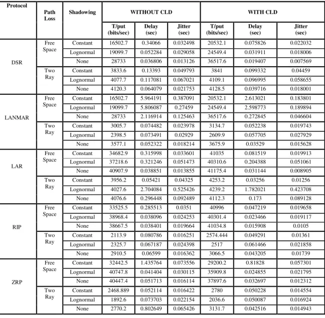
Fig. 3. Results for the other protocols are described in Table 1. As expected in the ideal model (free space with no shadowing) gives us the best performance. From Fig. 1 we can see that by using cross layer design throughput increases. In the free space propagation model assuming a circular static communication range, the average throughput observed is more than 3888.8 bits/sec in without cross layer design while it increases more than 4275.4 bits/sec in case of cross layer design.
Fig. 1 AODV variation in throughput
Fig.2 AODV variation in end to end delay
Fig.3 AODV variations in average jitter
Compared to this ideal scenario the results obtained in the free space propagation scenario with constant and lognormal shadowing effects are significantly lower (around 3585.8 bits/sec and 3427.2 bits/sec respectively) in without cross layer design while it increases (around 3777.9 bits/sec and 3916.7 bits/sec respectively) in with cross layer design. There is almost a 10% difference in performance between the ideal scenario and the free space with lognormal shadowing model in without cross layer design while in case of cross layer design its almost 8%. A similar trend is observed using the two-ray ground reflection model as well. The difference between the ideal scenario and the worst case scenario (Two Ray with lognormal shadowing) is more than 20%. This drastic reduction in performance does not bode well for the scheme in real world deployments. Similar trends are observed across all protocols and across the three metrics (with some exceptions). Further these results are without including additional factors that will affect the quality of the signal that is received such as fading effects and weather conditions. It is our observation that the main reason for this drastic difference in performance is the use of inefficient path metrics (such as hop count or distance) in the calculation of best routes to a certain destination that’s why the current surge in cross-layer design activity is motivated by the inability of the architecture to accommodate wireless links satisfactorily.
architectures either do not address the problems or do not sufficiently exploit the new opportunities created by the wireless links. Further, in energy constrained networks such as MANETs and sensor networks, the residual energy available in each node needs to be considered and included in the path metric value.
6. Conclusions And Future Work
This paper describes a comparison of cross layer design routing protocols methodology. Simulation results shows that the performance of physical layer (for path loss and shadowing properties) is drastically different as compared to the ideal scenario using cross layer deign. Also comparisons of throughput, average delay and average jitter between reference architecture and cross layer design methodology are done. In our future work we will extend this study to include other factors such as channel fading using the Raleigh and Rican fading models for this purpose using cross layer design. Further we hope to develop an efficient path metric that takes into account the current state of the channel and the quality of the link and to explore opportunistic routing strategies that a cross layer approach can make possible.
Table 1 Comparison of results between different Protocols
Protocol
Path Loss
Shadowing WITHOUT CLD WITH CLD
T/put (bits/sec) Delay (sec) Jitter (sec) T/put (bits/sec) Delay (sec) Jitter (sec) DSR Free Space
Constant 16502.7 0.34066 0.032498 20532.1 0.075826 0.022032
Lognormal 19099.7 0.052284 0.029058 24549.4 0.031911 0.018006
None 28733 0.036806 0.013126 36517.6 0.019407 0.007569
Two Ray
Constant 3833.6 0.13393 0.049793 3841 0.099332 0.04459
Lognormal 4077.7 0.117081 0.067021 4109.1 0.096995 0.058655
None 4120.3 0.064079 0.021753 4128.5 0.039716 0.018001
LANMAR
Free Space
Constant 16502.7 5.964191 0.387091 20532.1 2.613021 0.183801
Lognormal 19099.7 5.806087 0.27459 24549.4 2.598773 0.189894
None 28733 2.116914 0.125463 36517.6 0.272845 0.046604
Two Ray
Constant 3005.7 0.074482 0.023978 3134.7 0.052238 0.019743
Lognormal 2398.5 0.073491 0.02929 2609.9 0.057705 0.027929
None 3577.1 0.052322 0.018214 3675.9 0.03529 0.015628
LAR
Free Space
Constant 34682.9 0.315998 0.033601 41035 0.081519 0.019913
Lognormal 37218.6 0.321246 0.051473 40310.6 0.204388 0.051061
None 40907.9 0.038851 0.013855 41175.4 0.031144 0.008905
Two Ray
Constant 3956.2 0.05421 0.04325 4253.2 0.03256 0.01256
Lognormal 4027.6 2.704084 0.525426 4239.2 1.782021 0.423708
None 4076.6 0.296448 0.092489 4112.3 0.173 0.089128
RIP
Free Space
Constant 33525.5 0.285513 0.0351 40996 0.047219 0.019658
Lognormal 38968.4 0.038096 0.024253 40301.4 0.023466 0.019117
None 38667.5 0.038401 0.019664 41034.8 0.015908 0.0105
Two Ray
Constant 2113.9 0.080786 0.016251 2574.444 0.049291 0.01361
Lognormal 2325.7 0.067187 0.024398 2517 0.061466 0.021858
None 2910.5 0.06599 0.016362 3066.5 0.043205 0.01739
ZRP
Free Space
Constant 32442.5 1.435764 0.073556 29200.2 0.81828 0.057301
Lognormal 40747.8 0.041404 0.030115 35909.8 0.024855 0.021795
None 40447.4 0.051713 0.016114 37897.6 0.032697 0.012312
Two Ray
Constant 2468.889 0.052114 0.016422 2780 0.050228 0.014554
Lognormal 1892.6 0.073703 0.022154 2036.6 0.050087 0.016924
None 2770.2 0.802649 0.065426 3131.7 0.042516 0.014943
References
[1] J C-K Toh, “Ad Hoc Mobile Wireless Networks: Protocols and Systems”, Prentice Hall, New Jersey, 2002.
[3] V. Srivastava, “Cross-Layer Design: A Survey and the Road Ahead”, IEEE Communications Magazine, December 2005.
[4] C. Perkins and E. Royer, “Ad-Hoc On-Demand Distance Computing Systems and Applications, WMCSA ’99, New Orleans, February 1999.
[5] D. B. Johnson and D. A. Maltz, “Dynamic Source Routing in Ad-Hoc Wireless Networks”, Mobile Computing, Kluwer, 1996. [6] Y. Ko and N. Vaidya, “Location Aided Routing (LAR) in Mobile Ad Hoc Networks”, ACM/IEEE International Conference on Mobile
Computing and Networking, Dallas, MobiCom’98, October 1998.
[7] M. Gerla, X. Hong and G. Pei, “Landmark Routing for Large Ad Hoc Wireless Networks”, Proceedings of IEEE GLOBECOM 2000, San francisco,November 2000.
[8] C. Perkins, P. Bhagwat, “Highly Dynamic Destination-Sequenced Distance- Vector Routing (DSDV) for Mobile Computers”, Proceedings of ACM SIGCOMM’94 Conference on Communications architectures Protocols and Applications”, London, September 1994
[9] Z. Haas and M. Pearlman, “The Performance of Query Control Schemes for the Zone Routing Protocol”, ACM/IEEE Transactions on Networking, Volume 9, No.4, August 2001.45, Issue 3, June 2003 Page(s):51 - 82.
[10] Z. Haas, M. Pearlman, P. Samar, “The Bordercast Resolution Protocol (BRP) for Ad Hoc Networks”, IETF Internet Draft, draft-ietf-manetsone-brp-00.txt, January 2001.
[11] T.K. Sarkar et al., "A survey of various propagation models for mobilecommunication", IEEE Antennas and Propagation Magazine, Volume.