www.geosci-model-dev.net/8/1831/2015/ doi:10.5194/gmd-8-1831-2015
© Author(s) 2015. CC Attribution 3.0 License.
Verifications of the high-resolution numerical model and
polarization relations of atmospheric acoustic-gravity waves
N. M. Gavrilov1, S. P. Kshevetskii2, and A. V. Koval1
1Atmospheric Physics Department, Saint-Petersburg State University, Saint-Petersburg, Russia 2Theoretical Physics Department, Immanuel Kant Baltic Federal University, Kaliningrad, Russia Correspondence to:N. M. Gavrilov ([email protected])
Received: 26 September 2014 – Published in Geosci. Model Dev. Discuss.: 18 November 2014 Revised: 16 April 2015 – Accepted: 01 June 2015 – Published: 22 June 2015
Abstract.Comparisons of amplitudes of wave variations of atmospheric characteristics obtained using direct numerical simulation models with polarization relations given by con-ventional theories of linear acoustic-gravity waves (AGWs) could be helpful for testing these numerical models. In this study, we performed high-resolution numerical simulations of nonlinear AGW propagation at altitudes 0–500 km from a plane wave forcing at the Earth’s surface and compared them with analytical polarization relations of linear AGW theory. After some transition time te (increasing with alti-tude) subsequent to triggering the wave source, the initial wave pulse disappears and the main spectral components of the wave source dominate. The numbers of numerically sim-ulated and analytical pairs of AGW parameters, which are equal with confidence of 95 %, are largest at altitudes 30– 60 km att > te. At low and high altitudes and att < te,
num-bers of equal pairs are smaller, because of the influence of the lower boundary conditions, strong dissipation and AGW transience making substantial inclinations from conditions, assumed in conventional theories of linear nondissipative sta-tionary AGWs in the free atmosphere. Reasonable agree-ments between simulated and analytical wave parameters sat-isfying the scope of the limitations of the AGW theory prove the adequacy of the used wave numerical model. Signifi-cant differences between numerical and analytical AGW pa-rameters reveal circumstances when analytical theories give substantial errors and numerical simulations of wave fields are required. In addition, direct numerical AGW simulations may be useful tools for testing simplified parameterizations of wave effects in the atmosphere.
1 Introduction
Observations show the frequent presence of acoustic-gravity waves (AGWs) generating at tropospheric heights and prop-agating to the middle and upper atmosphere (e.g., Fritts and Alexander, 2003). These AGWs can break and produce turbulence and perturbations in the atmosphere (Gavrilov and Yudin, 1992; Gavrilov and Fukao, 1999). For example, sources of AGWs could be mesoscale turbulence and con-vection in the troposphere (e.g., Fritts and Alexander, 2003; Fritts et al., 2006). Turbulent AGW generation may have maxima at altitudes 9–12 km in the regions of tropospheric jet streams (Medvedev and Gavrilov, 1995).
Non-hydrostatic models are useful for direct numerical simulations of waves and turbulence in the atmosphere. For example, Baker and Schubert (2000) simulated non-linear AGWs in the atmosphere of Venus. They modeled waves in the atmospheric region with horizontal and ver-tical dimensions of 120 and 48 km, respectively. Fritts and Garten (1996), also Andreassen et al. (1998) and Fritts et al. (2009, 2011), simulated the instabilities of Kelvin and Helmholtz and turbulence produced by breaking atmospheric waves. These models simulate turbulence and waves in atmo-spheric regions with limited vertical and horizontal dimen-sions. The models exploited spectral methods and Galerkin-type series for converting partial differential equations (ver-sus time) into the ordinary differential equations for the spec-tral series components. Yu and Hickey (2007) and Liu et al. (2008) developed two-dimensional numerical models of atmospheric AGWs.
simulat-ing nonlinear AGWs ussimulat-ing a finite-difference scheme taksimulat-ing into account hydrodynamic conservation laws as described by Kshevetskii and Gavrilov (2005). This approach increases the stability of the numerical scheme and allows us to ob-tain non-smooth solutions of nonlinear wave equations. This permitted us to get generalized physically acceptable solu-tions to the equasolu-tions (Lax, 1957; Richtmayer and Morton, 1967). Gavrilov and Kshevetskii (2014a) created a three-dimensional version of this algorithm for simulating nonlin-ear AGWs in the atmosphere. They modeled waves produced by sinusoidal horizontally homogeneous wave forcing at the Earth’s surface.
Karpov and Kshevetskii (2014) used a similar numer-ical three-dimensional model to study AGW propagation from local non-stationary wave excitation at the Earth’s sur-face. They showed that infrasound going from tropospheric sources could provide substantial mean heating in the upper atmosphere. Dissipating nonlinear AGWs can also create ac-celerations of the mean flows in the middle atmosphere (e.g., Fritts and Alexander, 2003). However, details of the mean heating and mean flows created by non-stationary nonlinear AGWs in the atmosphere need further studies.
Numerical models of atmospheric AGWs require verifi-cations. For plane stationary wave components with small amplitudes, conventional linear theories (e.g., Gossard and Hooke, 1975) give the dispersion equation and polarization relations, which connect wave frequency, vertical and hor-izontal wave numbers and ratios of amplitudes of different wave field variations. One can expect that such relations could exist between corresponding parameters of the numer-ical model solutions. Therefore, theoretnumer-ical polarization rela-tions could be useful for verifying direct simulation models of atmospheric AGWs.
In this paper, using the high-resolution numerical three-dimensional model by Gavrilov and Kshevetskii (2014a, b), we made comparisons of calculated ratios of amplitudes of different wave fields with polarization relations given by the conventional linear AGW theory. We considered simple AGW forcing by plane wave oscillations of vertical velocity at the surface, which is similar to the assumptions made in analytical wave theory. We found height regions of the atmo-sphere where numerical results agree with analytical ones, and regions of their substantial disagreement.
Theoretical dispersion equation and polarization relations are widely used for developing simplified parameterizations of AGW dynamical and thermal effects in the general cir-culation models of the middle atmosphere. Therefore, com-parisons of numerically modeled and analytical polarization relations are useful for both verifications of numerical mod-els, and obtaining limits of analytical relation applicability and for verifying AGW parameterizations.
2 Numerical model
The three-dimensional numerical AGW model calculates ve-locity componentsu,v, andw along horizontal (x,y) and vertical,z, axes, respectively. The model also calculates de-partures of pressurep′, temperatureT′, and densityρ′from background hydrostatic stationary fieldsp0,T0, andρ0, re-spectively. Gavrilov and Kshevetskii (2014a) described the set of hydrodynamic nonlinear equations used in the model. The set includes equations of continuity, momentum and heat balance. At the upper boundaryz=500 km, the conditions involve zero vertical gradients of perturbations of tempera-ture, pressure, density and horizontal velocity, and zero ver-tical velocity. At the Earth’s surface, the lower boundary con-ditions consist of zero perturbations of temperature, pressure, density and horizontal velocity (see Gavrilov and Kshevet-skii, 2013, 2014a, b). In this study, we assume horizontal pe-riodicity of wave solutions:
r(x, y, z, t )=r(x+Lx, y+Ly, z, t ), (1)
where r denotes any of the calculated variables, and
Lx=mλx, Ly=nλy are the horizontal dimensions of the considered atmospheric region, m and n are integer con-stants, and λx and λy are wavelengths along horizontal
axes x and y, respectively. Variations of vertical velocity
w0=w(x, y) at the ground z=0 generate AGWs in the model.
The used numerical scheme is analogous to the two-dimensional algorithm described by Kshevetskii and Gavrilov (2005). It is a modification of the method by Lax and Wendroff (1960). This algorithm involves the conserva-tion laws of momentum, mass and energy. The main dif-ferences of our scheme from the classical Lax and Wen-droff (1960) algorithm are the implicit approximating equa-tions of hydrodynamics at the first half step in time, which diminish errors of description of acoustic waves (Kshevet-skii, 2001a, b, c).
We use a numerical scheme similar to the two-dimensional algorithm developed by Kshevetskii and Gavrilov (2005). Used hydrodynamic equations (see Gavrilov and Kshevet-skii, 2013, 2014a) can be presented in the conservation law forms
∂s ∂t +
∂X(s)
∂x +
∂Y (s)
∂y +
∂Z(s)
∂z =0, (2)
Eq. (2) with the second-order finite-difference analog
si,j,kn+1−sni,j,k
1t +
Xi+n+11//22,j,k−Xin+−11//22,j,k
1x
+
Yi,jn++1/12/2,k−Yi,jn+−1/1/22,k
1y
+
Zi.j.k+n+1/21/2−Zn+i,j,k−1/21/2
1z =0, (3)
wheren,i,j,kand1t,1x,1y,1zare the grid node num-bers and grid spacing in t, x,y, and z, respectively. This algorithm gives possibilities to select physically appropri-ate solutions of the equations (Lax, 1957; Richtmayer and Morton, 1967). It keeps the numerical scheme stability and allows us consideration of non-smooth solutions of nonlin-ear AGW equations. In addition, we exploit a staggered grid, where temperature, pressure and density are specified at the same nodes, but for the velocity componentsu,v,wthe mesh points are half grid spacing shifted along axesx,y, andz, re-spectively. To computesn+1/2at the first time half step, we apply the implicit equation
2
sn+i,j,k1/2−si,j,kn
1t +
Xn+i+11//22,j,k−Xi−n+11//22,j,k
1x
+
Yi,j+n+11/2/2,k−Yi,jn+−1/12/2,k
1y
+Z
n+1/2
i.j.k+1/2−Z
n+1/2
i,j,k−1/2
1z =0. (4)
This substantially complicates simulations, but Kshevet-skii (2001a, b, c) found that such structures of finite-difference schemes do not accumulate errors caused by acoustic waves.
In this study, we employ vertical profiles of background
T0,ρ0, andp0given by the model of standard atmosphere MSIS-90 (Hedin, 1991) for average geomagnetic activity in January. The average spacing of the height grid is about 170 m, but it varies from 12 m near the ground (because of high gradients in the boundary layer) to about 1.2 km at al-titudes of about 500 km, depending on inhomogeneities of vertical temperature profiles. The horizontal grid spacing is 1/60 of horizontal wavelengths taken in the wave source Eq. (2). Time spacing is automatically determined to guar-antee stability of the numerical algorithm and is equal to 0.14 and 0.24 s for AGWs analyzed in this study with period
τ =2×10³s and horizontal phase speeds 30 and 100 m s−1, respectively.
The numerical model involves kinematic molecular heat conductivity and viscosity, increasing versus altitude in-versely proportional to the background density. We also include background turbulent heat conductivity and vis-cosity, taking their vertical profiles with the maxima of 10 m2s−1 near the ground and at altitude of 100 km and
the minimum of∼0.1 m2s−1in the stratosphere (Gavrilov, 2013). The model does not include some effects, for ex-ample, wave dissipation caused by ion drag and radiative heat exchange, which are less important for modeling high-frequency AGWs.
3 AGW polarization relations
The comparisons considered in this paper used relations ob-tained from a theoretical model of monochromatic AGWs in the plain rotating atmosphere. Conventional linear theories suppose that wave componentsv′,p′,ρ′, andT′ are small
deviations from stationary background valuesv0,p0,ρ0, and
T0. In agreement with Hines (1960), Beer (1974), and Msuno and Shimazaki (1981), we can look for solutions to at-mospheric wave equations for AGW spectral components in the following form
u′
U =
v′
V =
w′
W =
p′ p0P
= ρ
′
ρ0R = T
′
T02
=
rp
0s p0
ei(σ t+φ), φ= −kx−mz, (5)
wherep0s is the surface pressure; axis x is directed along
horizontal wave phase velocity;σ,k andmare frequency, horizontal and vertical wave numbers; andU,V,W,P,R
and2are complex amplitudes of respective values. Assum-ing homogeneity ofv0 andT0, one can obtain (see Hines,
1960, and Beer, 1974) a dispersion equation relating fre-quency and wave numbers, which can be written in the form of
m2=N 2−ω2
ω2−f2k
2−ω2a−ω2
c2 , (6)
wheref is the Coriolis parameter,Nis the isothermal Brunt– Vaisala frequency,cis the sound speed, andωais the high-est frequency of acoustic waves,ω=σ−ku0. Beer (1974) found that Eq. (6) could be an appropriate approximation for slowly varying background temperature and wind if one uses the following expressions:
N2= g
T0
(∂T0
∂z +γa); ω
2 a=
c2
4H2(1+2
∂H
∂z), (7)
whereγa=g/cp,g is the acceleration by gravity,H is the
atmospheric scale height, andcpis the heat capacity at
con-stant pressure. Applying the technique by Beer (1974), we can get the following polarization relations:
U∝ωkc2(m−iŴ), W∝ω(ω2−f2−k2c2),
V ∝if kc2(m−iŴ), P ∝γ (ω2−f2)(m−iŴ),
R∝(ω2−f2)(m−iα)+ik2c2N2/g,
2∝(γ−1)(ω2−f2)(m+iα)−ik2c2N2/g, (8) whereα=1/(2H );Ŵ=(2−γ )/(2γ H );γ=cp/cv.
but gives the opportunity to find their ratios. At f =0, Eq. (8) are equivalent to the polarization relations obtained by Hines (1960). In a nondissipative atmosphere, according to Eq. (5), AGW amplitudes should grow with altitude, so that
W =W0
p
p0s/p0. (9)
An important AGW characteristic is the wave momentum flux, the vertical component of which,Fmz, is as follows: Fmz=ρ0hu′w′i =ρ0Re(U W∗)/2, (10) where signh idenotes averaging over the wave period.
4 Comparisons of the numerical model and polarization relations
In this study, using the high-resolution nonlinear numeri-cal model described in Sect. 2, we simulated hydrodynamic fields produced by spectral AGW components and compared ratios of their amplitudes with those predicted by the analyt-ical polarization relations Eqs. (7) and (8). To make simula-tions matching the linear AGW theory (see Eq. 5), we used nonlinear AGWs with forms of plane waves and suppose hor-izontally periodical distributions of vertical velocity at the Earth’s surface moving along axisxof the form of
(w)z=0=W0cos[k(x−cxt )], (11)
where k=2π/λx and cx are horizontal wave-number and phase speed along the horizontal axisxin the direction of the wave propagation;W0is the amplitude. Equation (11) repre-sents the plane wave of vertical velocity at the lower bound-ary, which may correspond to spectral components of con-vective and turbulent AGW sources (Townsend, 1965, 1966). Medvedev and Gavrilov (1995) studied AGW generation caused by nonlinear interactions in meteorological and tur-bulent atmospheric processes. They found a variety of wave-lengths, amplitudes and other parameters of created AGWs. In this paper, we describe simulations for wave modes with
cx=30 m s−1 and cx=100 m s−1 with unchanged period
τ =2×10³s and amplitudesW0=0.3 cm s−1. The modeling was performed beginning from the MSIS initial state (zero wave fields) and the windless background flow att=0, when the wave source Eq. (11) was triggered at the lower boundary. Gavrilov and Kshevetskii (2014a, b) demonstrated that, af-ter triggering the wave source att=0, fast acoustic and very long gravity wave modes would quickly reach very high alti-tudes. Simulations demonstrate that, in the horizontally peri-odic approximation of Eq. (1), these initial pulses can reach altitudes of 100 km and higher in a few minutes and form quasi-vertical wave fronts analogous to those in Fig. 1a, b, c of the paper by Gavrilov and Kshevetskii (2013, 2014a). These initial waves dissipate because of molecular viscosity and heat conduction. When time increases, more and more of
the waves with longer vertical wavelengths are taken away by dissipation; therefore, vertical wavelengths should decrease in time at a given height in the middle atmosphere (Heale et al., 2014). After some transition time, initial AGW wave modes disappear and wave vertical structure matches the main spectral component of the wave source (Eq. 11) with horizontal wave numberkand phase speedcx.
To estimate AGW amplitudes in the numerical model so-lution, we calculated standard deviations of the correspond-ing wave fields over all nodes of the horizontal grid at the considered altitude. For the sinusoidal wave component, this standard deviation is equal to a half AGW amplitude. There-fore, ratios of amplitudes of horizontally homogeneous sta-tionary sinusoidal AGWs should be equal to the ratios of the corresponding standard deviations. Simulated standard de-viations of wave fields in horizontal planes located at dif-ferent heights grow in time throughout transition intervals after activating the wave forcing and then tend to constant values different at each height (see Gavrilov and Kshevet-skii, 2014b). In the horizontally periodical approximation of Eq. (1), these standard deviations are approximately equal to half wave amplitudes at larget, when the AGW process tends to become quasi-stationary. For a plane spectral AGW component with vertical wavelengthλz, the vertical group
velocity iscgz≈λz/τ, and the time of its energy arriving
at altitudeziste=z/cgz. For the considered main spectral components of the wave source (Eq. 11) withτ=2×10³s and average λz∼10 km for cx=30 m s−1, λz∼35 km for cx=100 m s−1. Therefore, one can get te/τ=z/λz∼1, 6,
10 and te/τ∼0.3, 1.7, 2.9 at heights 10, 60, and 100 km,
respectively, for bothcx. Thus, lengths of the transition
in-tervals are longer for smallercx. These intervals grow with
altitude and may be longer than ten wave periods at a height of 100 km.
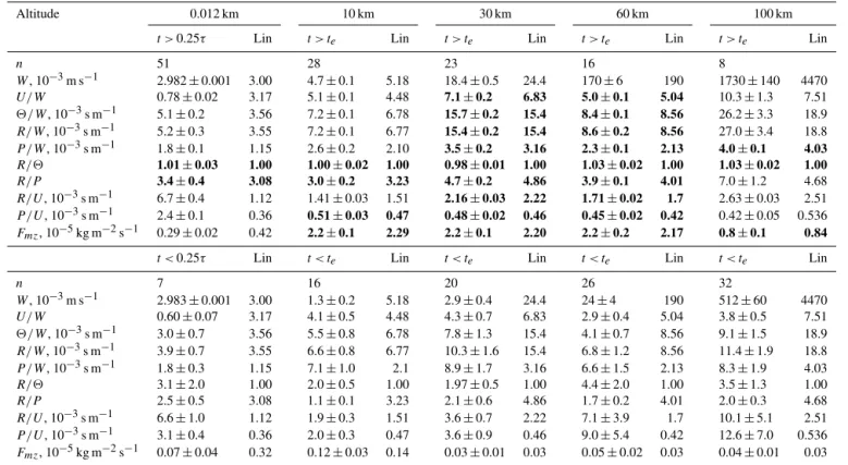
Table 1 represents standard deviations at different alti-tudes calculated with the numerical model and with ana-lytical polarization relations and their ratios for AGW with
cx=30 m s−1. Table 1 contains simulated SDs at each alti-tude averaged overn model outputs during the initial tran-sient intervalt < te (bottom part of Table 1) and for
quasi-stationary wavest > te (upper part of Table 1). Respective
data numbersn for each altitude are presented in Table 1. Respective values obtained from analytical linear AGW the-ory (see Sect. 3) are calculated using average background values and are placed in the columns labeled “Lin” at each altitude in Table 1. Consideration of Fig. 5 of the paper by Gavrilov and Kshevetskii (2014b) shows that standard devia-tions of wave fields simulated with the numerical model vary in time due to definite variations and irregular perturbations. Standard deviations of each average numerically simulated parameter are given in Table 1.
Table 1.Standard deviations and their ratios for AGW withcx=30 m s−1calculated with the numerical model and with analytical polar-ization relations (labeled as Lin) at different altitudes averaged over the initial transient intervalt < teand for quasi-stationary wavest > te. Bold font shows the data pairs equal to probabilities larger than 95 %.
Altitude 0.012 km 10 km 30 km 60 km 100 km
t >0.25τ Lin t > te Lin t > te Lin t > te Lin t > te Lin
n 51 28 23 16 8
W, 10−3m s−1 2.982±0.001 3.00 4.7±0.1 5.18 18.4±0.5 24.4 170±6 190 1730±140 4470
U/W 0.78±0.02 3.17 5.1±0.1 4.48 7.1±0.2 6.83 5.0±0.1 5.04 10.3±1.3 7.51
2/W, 10−3s m−1 5.1±0.2 3.56 7.2±0.1 6.78 15.7±0.2 15.4 8.4±0.1 8.56 26.2±3.3 18.9
R/W, 10−3s m−1 5.2±0.3 3.55 7.2±0.1 6.77 15.4±0.2 15.4 8.6±0.2 8.56 27.0±3.4 18.8
P /W, 10−3s m−1 1.8±0.1 1.15 2.6±0.2 2.10 3.5±0.2 3.16 2.3±0.1 2.13 4.0±0.1 4.03
R/2 1.01±0.03 1.00 1.00±0.02 1.00 0.98±0.01 1.00 1.03±0.02 1.00 1.03±0.02 1.00
R/P 3.4±0.4 3.08 3.0±0.2 3.23 4.7±0.2 4.86 3.9±0.1 4.01 7.0±1.2 4.68
R/U, 10−3s m−1 6.7±0.4 1.12 1.41±0.03 1.51 2.16±0.03 2.22 1.71±0.02 1.7 2.63±0.03 2.51
P /U, 10−3s m−1 2.4±0.1 0.36 0.51±0.03 0.47 0.48±0.02 0.46 0.45±0.02 0.42 0.42±0.05 0.536
Fmz, 10−5kg m−2s−1 0.29±0.02 0.42 2.2±0.1 2.29 2.2±0.1 2.20 2.2±0.2 2.17 0.8±0.1 0.84
t <0.25τ Lin t < te Lin t < te Lin t < te Lin t < te Lin
n 7 16 20 26 32
W, 10−3m s−1 2.983±0.001 3.00 1.3±0.2 5.18 2.9±0.4 24.4 24±4 190 512±60 4470
U/W 0.60±0.07 3.17 4.1±0.5 4.48 4.3±0.7 6.83 2.9±0.4 5.04 3.8±0.5 7.51
2/W, 10−3s m−1 3.0±0.7 3.56 5.5±0.8 6.78 7.8±1.3 15.4 4.1±0.7 8.56 9.1±1.5 18.9
R/W, 10−3s m−1 3.9±0.7 3.55 6.6±0.8 6.77 10.3±1.6 15.4 6.8±1.2 8.56 11.4±1.9 18.8
P /W, 10−3s m−1 1.8±0.3 1.15 7.1±1.0 2.1 8.9±1.7 3.16 6.6±1.5 2.13 8.3±1.9 4.03
R/2 3.1±2.0 1.00 2.0±0.5 1.00 1.97±0.5 1.00 4.4±2.0 1.00 3.5±1.3 1.00
R/P 2.5±0.5 3.08 1.1±0.1 3.23 2.1±0.6 4.86 1.7±0.2 4.01 2.0±0.3 4.68
R/U, 10−3s m−1 6.6±1.0 1.12 1.9±0.3 1.51 3.6±0.7 2.22 7.1±3.9 1.7 10.1±5.1 2.51
P /U, 10−3s m−1 3.1±0.4 0.36 2.0±0.3 0.47 3.6±0.9 0.46 9.0±5.4 0.42 12.6±7.0 0.536
Fmz, 10−5kg m−2s−1 0.07±0.04 0.32 0.12±0.03 0.14 0.03±0.01 0.03 0.05±0.02 0.03 0.04±0.01 0.03
of two irregular quantities (Rice, 2006). Approximately, the probability of equity of two respective average values in Ta-ble 1 is larger 95 %, if the difference between them is less than 1.96 multiplied by the standard deviation of the average value (Rice, 2006). In this study, we considered only cases where the standard deviations in Table 1 are smaller than 0.15 of the respective average values. Pairs of AGW parame-ters, which we can consider equal with confidence larger than 95 %, are marked with bold font in Table 1. The numbers of those pairs are largest in the upper part of Table 1 at altitudes 30 and 60 km, which correspond to quasi-stationary AGWs in the free atmosphere considered in conventional AGW the-ory described in Sect. 3. Reasonable agreements between simulated and analytical wave parameters in atmospheric re-gions, which correspond to the scope of the limitations of the nondissipative linear AGW theory, may be considered as evi-dence of adequate descriptions of wave processes by the used nonlinear numerical model.
Many numerically simulated AGW parameters do not match the respective analytical values in Table 1. No matches are in the bottom part of Table 1, which corresponds to the initial transition time interval. Gavrilov and Kshevet-skii (2014b) showed that vertical structures of transient waves are different from those predicted by the linear AGW theory during the transition interval after activating the sur-face wave source Eq. (11). The bottom part of Table 1 shows
that numerically simulated wave amplitudeWis smaller than that predicted by AGW theory at high altitudes, because these values refer to smallt < te, when the energy of the main
wave component does not yet reach the considered altitude. Numerical and analytical amplitude ratios are also substan-tially different in the bottom part of Table 1 fort < te.
In the upper part of Table 1 for quasi-stationary AGWs att > te, the numerically simulated AGW amplitudesW are
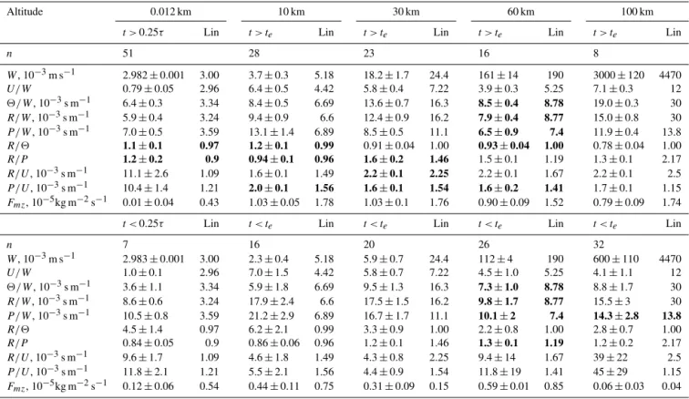
agree-Table 2.Same as Table 1 but for AGW withcx=100 m s−1.
Altitude 0.012 km 10 km 30 km 60 km 100 km
t >0.25τ Lin t > te Lin t > te Lin t > te Lin t > te Lin
n 51 28 23 16 8
W, 10−3m s−1 2.982±0.001 3.00 3.7±0.3 5.18 18.2±1.7 24.4 161±14 190 3000±120 4470
U/W 0.79±0.05 2.96 6.4±0.5 4.42 5.8±0.4 7.22 3.9±0.3 5.25 7.1±0.3 12
2/W, 10−3s m−1 6.4±0.3 3.34 8.4±0.5 6.69 13.6±0.7 16.3 8.5±0.4 8.78 19.0±0.3 30
R/W, 10−3s m−1 5.9±0.4 3.24 9.4±0.9 6.6 12.4±0.9 16.2 7.9±0.4 8.77 15.0±0.8 30
P /W, 10−3s m−1 7.0±0.5 3.59 13.1±1.4 6.89 8.5±0.5 11.1 6.5±0.9 7.4 11.9±0.4 13.8
R/2 1.1±0.1 0.97 1.2±0.1 0.99 0.91±0.04 1.00 0.93±0.04 1.00 0.78±0.04 1.00
R/P 1.2±0.2 0.9 0.94±0.1 0.96 1.6±0.2 1.46 1.5±0.1 1.19 1.3±0.1 2.17
R/U, 10−3s m−1 11.1±2.6 1.09 1.6±0.1 1.49 2.2±0.1 2.25 2.2±0.1 1.67 2.2±0.1 2.5
P /U, 10−3s m−1 10.4±1.4 1.21 2.0±0.1 1.56 1.6±0.1 1.54 1.6±0.2 1.41 1.7±0.1 1.15
Fmz, 10−5kg m−2s−1 0.01±0.04 0.43 1.03±0.05 1.78 1.03±0.1 1.76 0.90±0.09 1.52 0.79±0.09 1.74
t <0.25τ Lin t < te Lin t < te Lin t < te Lin t < te Lin
n 7 16 20 26 32
W, 10−3m s−1 2.983±0.001 3.00 2.3±0.4 5.18 5.9±0.7 24.4 112±4 190 600±110 4470
U/W 1.0±0.1 2.96 7.0±1.5 4.42 5.8±0.7 7.22 4.5±1.0 5.25 4.1±1.1 12
2/W, 10−3s m−1 3.6±1.1 3.34 5.9±1.8 6.69 9.5±1.3 16.3 7.3±1.0 8.78 8.8±1.7 30
R/W, 10−3s m−1 8.6±0.6 3.24 17.9±2.4 6.6 17.5±1.5 16.2 9.8±1.7 8.77 15.5±3 30
P /W, 10−3s m−1 10.5±0.8 3.59 21.2±2.9 6.89 16.7±1.7 11.1 10.1±2 7.4 14.3±2.8 13.8
R/2 4.5±1.4 0.97 6.2±2.1 0.99 3.3±0.9 1.00 2.2±0.8 1.00 2.8±0.7 1.00
R/P 0.84±0.05 0.9 0.86±0.06 0.96 1.2±0.1 1.46 1.3±0.1 1.19 1.2±0.2 2.17
R/U, 10−3s m−1 9.6±1.7 1.09 4.6±1.8 1.49 4.3±0.8 2.25 9.4±14 1.67 39±22 2.5
P /U, 10−3s m−1 11.8±2.1 1.21 5.5±2.1 1.56 4.4±0.9 1.54 11.8±19 1.41 45±29 1.15
Fmz, 10−5kg m−2s−1 0.12±0.06 0.54 0.44±0.11 0.75 0.31±0.09 0.15 0.59±0.01 0.85 0.06±0.03 0.04
ments exist between numerical and analytical values of the ratioR/2≈1 at all altitudes.
Table 1 reveals the numerically simulated AGW momen-tum fluxes Fmz Eq. (10) calculated as ρ0hu′w′i averaged over horizontal planes at fixed altitudes and over respective time intervals. For comparisons, Table 1 also contains mo-mentum fluxes Fmz given by Eq. (10) and calculated from numerically simulated amplitudesW andU. The upper part of Table 1 shows that, att > te, wave momentum fluxFmzis
almost constant at altitudes 10–60 km due to relatively small dissipation and reflection of wave energy. At an altitude of 100 km, wave dissipation increases andFmz decreases,
pro-ducing strong wave accelerations of the mean flow, which are proportional to the vertical gradient of Fmz. In the
bot-tom part of Table 1 fort < te, values ofFmzare much smaller
than respectiveFmzvalues fort > te, because during the
ini-tial transition interval, the energy of the main AGW modes of the wave source (Eq. 11) does not yet reach high altitudes. Table 2 is the same as Table 1, but for AGW components withcx=100 m s−1, which has a longer vertical wavelength. In the upper part of Table 2 fort > te, we have a smaller num-ber of pairs equal with confidence 95 % (marked with bold font) than that in the upper part of Table 1. This may be con-nected to the stronger influence of vertical inhomogeneities of background temperature profiles on a faster AGW with a longer vertical wave number and with larger partial reflection of faster AGW energy. Stronger reflections lead to smaller
amplitudesW at altitudes below 100 km in the upper part of Table 2 compared to that in Table 1. On the other hand,W
at altitude 100 km in the upper part of Table 2 is larger than that in Table 1 due to smaller dissipation of longer AGWs. Therefore, waves with longer vertical wavelengths can prop-agate faster from the surface to the upper layers and dissipate less in the middle atmosphere, where they can have ampli-tudes larger than those for shorter vertical wavelength AGWs (see Gavrilov and Kshevetskii, 2014b). Similar to Table 1, we have larger amounts of equal (with 95 % confidence) numer-ically simulated and analytical AGW parameters at altitudes 30 and 60 km. At low and high altitudes and att < te(in the
bottom part of Table 2), numbers of equal pairs are smaller due to the influence of the lower boundary conditions, larger dissipation and AGW transience, respectively.
sources due to higher nonlinear effects and faster growths in the wave-induced jet streams above 100 km. To get better agreements, improved analytical AGW theories taking into account transient processes, high wave dissipation and fast changes in background fields are required.
In the areas of Tables 1 and 2, where numerical and analyt-ical parameters are close, one can use analytanalyt-ical formulae for descriptions and estimations of the wave fields. Opposite to that, areas of substantial differences between numerical and analytical AGW parameters in Tables 1 and 2 reveal regions where numerical simulations are required.
Relations of linear AGW theory are frequently used for simplified parameterizations of AGW dynamical and ther-mal effects for their use in the numerical models of atmo-spheric general circulations (e.g., Lindzen, 1981; Holton, 1983; Gavrilov and Yudin, 1992, etc.). Similar parameteriza-tions are also being developed for highly dissipative AGWs in the upper atmosphere (e.g., Vadas and Fritts, 2005; Yigit et al., 2008). Sometimes, different parameterizations give dif-ferent results. Direct numerical simulation models of atmo-spheric AGWs may be useful tools for testing and verifying simplified parameterizations of wave effects.
5 Conclusions
In this study, we performed high-resolution numerical sim-ulations of nonlinear AGW propagation to the middle and upper atmosphere from a plane wave forcing at the Earth’s surface and compared them with analytical polarization rela-tions of linear AGW theory. Such comparisons may be used for verifications of numerical models of atmospheric AGWs. Numerical simulations show that, after triggering the wave source Eq. (11) at t=0, fast acoustic and very long grav-ity wave modes would quickly reach very high heights. Af-ter some transition time te (increasing with altitude),
ini-tial AGW wave modes disappear and wave vertical struc-ture matches the main spectral component of the wave source Eq. (11) with horizontal wave numberkand phase speedcx.
The numbers of numerically simulated and analytical pairs of AGW parameters, which are equal with confidence 95 %, are largest at altitudes 30 and 60 km at t > te. At low and high altitudes and at t < te, numbers of equal pairs are smaller, because of the influence of the lower boundary conditions, larger dissipation and AGW transience, which can produce substantial inclinations from conditions, assumed in conven-tional theories of linear nondissipative stationary AGWs in the free atmosphere.
Reasonable agreements between numerically simulated and analytical wave parameters in atmospheric regions, which correspond to the scope of the limitations of the AGW theory, may be considered as evidence of adequate descrip-tions of wave processes by the used nonlinear numerical model. Areas of substantial differences between numerical and analytical AGW parameters reveal atmospheric regions,
where analytical theories give substantial errors and numer-ical simulation of wave fields is required. Direct numeri-cal simulation models of atmospheric AGWs may be useful tools for testing and verifying simplified parameterizations of wave effects.
Acknowledgements. This work was partly supported by the Russian Basic Research Foundation, by the Russian Scientific Foundation (grant 14-17-00685), and by the Ministry of Education and Science of the Russian Federation (contract 3.1127.2014/K).
Edited by: O. Marti
References
Andreassen, O., Hvidsten, O., Fritts, D., and Arendt, S.: Vorticity dynamics in a breaking internal gravity wave. Part 1. Initial in-stability evolution, J. Fluid. Mech., 367, 27–46, 1998.
Baker, D. and Schubert, G.: Convectively generated internal gravity waves in the lower atmosphere of Venus. Part II: mean wind shear and wave-mean flow interaction, J. Atmos. Sci., 57, 200–215, 2000.
Beer, T.: Atmospheric waves, Adam Hilder, London, 1974. Fritts, D. C. and Alexander, M. J.: Gravity wave dynamics and
effects in the middle atmosphere, Rev. Geophys., 41, 1003, doi:10.1029/2001RG000106, 2003.
Fritts, D. C. and Garten, J. F.: Wave breaking and transition to tur-bulence in stratified shear flows, J. Atmos. Sci., 53, 1057–1085, 1996.
Fritts, D. C., Vadas, S. L., Wan, K., and Werne, J. A.: Mean and variable forcing of the middle atmosphere by gravity waves, J. Atmos. Sol.-Terr. Phys., 68, 247–265, 2006.
Fritts, D. C., Wang, L., Werne, J., Lund, T., and Wan, K.: Gravity wave instability dynamics at high Reynolds numbers. Part II: tur-bulence evolution, structure, and anisotropy, J. Atmos. Sci., 66, 1149–1171, 2009.
Fritts, D. C., Franke, P. M., Wan, K., Lund, T., and Werne, J.: Com-putation of clear air radar backscatter from numerical simula-tions of turbulence: 2. Backscatter moments throughout the life-cycle of a Kelvin-Helmholtz instability, J. Geophys. Res., 116, D11105, doi:10.1029/2010JD014618, 2011.
Gavrilov, N. M.: Estimates of turbulent diffusivities and energy dissipation rates from satellite measurements of spectra of stratospheric refractivity perturbations, Atmos. Chem. Phys., 13, 12107–12116, doi:10.5194/acp-13-12107-2013, 2013.
Gavrilov, N. M. and Fukao, S.: A comparison of seasonal variations of gravity wave intensity observed by the MU radar with a theo-retical model, J. Atmos. Sci., 56, 3485–3494, doi:10.1175/1520-0469(1999)056<3485:ACOSVO>2.0.CO;2, 1999.
Gavrilov, N. M. and Kshevetskii, S. P.: Numerical modeling of prop-agation of breaking nonlinear acoustic-gravity waves from the lower to the upper atmosphere, Adv. Space Res., 51, 1168–1174, doi:10.1016/j.asr.2012.10.023, 2013.
Gavrilov, N. M. and Kshevetskii, S. P.: Three-dimensional numer-ical simulation of nonlinear acoustic-gravity wave propagation from the troposphere to the thermosphere, Earth Planets Space, 66, 88, doi:10.1186/1880-5981-66-88, 2014b.
Gavrilov, N. M. and Yudin, V. A.: Model for coefficients of turbu-lence and effective Prandtl number produced by breaking gravity waves in the upper atmosphere, J. Geophys. Res., 97, 7619–7624, doi:10.1029/92JD00185, 1992.
Gavrilov, N. M., Fukao, S., Nakamura, T.: Peculiarities of interan-nual changes in the mean wind and gravity wave characteristics in the mesosphere over Shigaraki, Japan, Geophys. Res. Lett., 26, 2457–2460, doi:10.1029/1999GL900559, 1999.
Gossard, E. E. and Hooke, W. H.: Waves in the atmosphere, Elsevier Sci. Publ. Co., Amsterdam-Oxford-New York, 1975.
Heale, C. J., Snively, J., Hickey, M. P., and Ali, C.: Thermospheric dissipation of upward propagating gravity wave packets, J. Geo-phys. Res., 119, 3857–387, doi:10.1002/2013JA019387, 2014. Hedin, A. E.: Neutral atmosphere empirical model from the surface
to lower exosphere MSISE-90, extension of the MSIS thermo-sphere model into the middle and lower atmothermo-sphere, J. Geophys. Res., 96, 1159–1172, 1991.
Hines, C. O.: Internal atmospheric gravity waves at ionospheric heights, Can. J. Phys., 38, 1441–1481, 1960.
Holton, J. R.: The influence of gravity wave breaking on the general circulation of the middle atmosphere, J. Atmos. Sci., 40, 2497– 2507, 1983.
Karpov, I. V. and Kshevetskii, S. P.: Formation of large-scale distur-bances in the upper atmosphere caused by acoustic gravity wave sources on the Earth’s surface, Geomagn. Aeronomy, 54, 553– 562, 2014.
Kshevetskii, S. P.: Modelling of propagation of internal gravity waves in gases, Comp. Math. Math. Phys., 41, 295–310, 2001a. Kshevetskii, S. P.: Analytical and numerical investigation of
non-linear internal gravity waves, Nonnon-linear Proc. Geoph., 8, 37–53, 2001b.
Kshevetskii, S. P.: Numerical simulation of nonlinear internal grav-ity waves, Comp. Math. Math. Phys., 41, 1777–1791, 2001c.
Kshevetskii, S. P. and Gavrilov, N. M.: Vertical propagation, break-ing and effects of nonlinear gravity waves in the atmosphere, J. Atmos. Sol.-Terr. Phys., 67, 1014–1030, 2005.
Lax, P. D.: Hyperbolic systems of conservation laws, Comm. Pure Appl. Math., 10, 537–566, 1957.
Lax, P. D. and Wendroff, B.: Hyperbolic systems of conservation laws, Comm. Pure Appl. Math., 13, 217–237, 1960.
Lindzen, R. S.: Turbulence and stress owing to gravity wave and tidal breakdown, J. Geophys. Res., 86, 9707–9714, 1981. Liu, X., Xu, J., Liu, H.-L., and Ma, R.: Nonlinear interactions
be-tween gravity waves with different wavelengths and diurnal tide, J. Geophys. Res., 113, D08112, doi:10.1029/2007JD009136, 2008.
Matsuno, T. and Shimazaki, T.: Lectures on Atmospheric Science, 3., Stratosphere-Mesosphere, Univ. Tokyo Press, Tokyo, 1981. Medvedev, A. S. and Gavrilov, N. M.: The nonlinear mechanism of
gravity wave generation by meteorological motions in the atmo-sphere, J. Atmos. Terr. Phys., 57, 1221–1231, 1995.
Rice, J. A.: Mathematical Statistics and Data Analysis, 3rd Edn., Duxbury Advanced, 2006.
Richtmayer, R. R. and Morton, K. W.: Difference methods for initial-value problems, Intersci. Publ., New York, 1967. Townsend, A. A.: Excitation of internal waves by a turbulent
bound-ary layer, J. Fluid. Mech. 22, 241–252, 1965.
Townsend, A. A.: Internal waves produced by a convective layer, J. Fluid. Mech., 24, 307–319, 1966.
Vadas, S. L. and Fritts, D. C.: Thermospheric responses to gravity waves: Influences of increasing viscosity and thermal diffusiv-ity, J. Geophys. Res., 110, D15103, doi:10.1029/2004JD005574, 2005.
Yigit, E., Aylward, A. D., and Medvedev, A. S.: Parameterization of the effects of vertically propagating gravity waves for thermo-sphere general circulation models: sensitivity study, J. Geophys. Res., 113, D19106, doi.10.1029/2008JD010135, 2008.