Abstract— In this paper, a new adaptation of spreadsheet heuristic for stochastic demand environment is presented. The simplicity of application of spreadsheet method and its efficiency enable us to consider its modified version for the joint replenishment problem under stochastic demand. The principle of the procedure is to find a balance between the replenishment and holding costs for jointly replenished items. The heuristic performance is tested on real business data and we found out that it performs well in comparison with well known RAND heuristic. Owing to the simplicity and effectiveness of the proposed algorithm, we believe that it can be applicable in retail industry.
Index Terms— Spreadsheet heuristic, Stochastic demand environments, Joint replenishment problem, Business data.
I. INTRODUCTION
Replenishment policies are highly important in inventory management area. In the literature and practice, there are many types of inventory models dealing with multi-product environments [1]. The objective of an inventory model is generally finding the trade-off between replenishment cost and holding cost.
The objective of this article is present a new adaptation of the spreadsheet heuristic for stochastic demand environment under joint replenishment policy. Real world data is used and tested in order to measure the effectiveness of the proposed method.
The numerical data used in the application belongs to a worldwide known consumer electronic company and the joint replenishment strategy is determined to minimize total costs. High technology industries have several unique characteristics in terms of supply chain management. First and foremost, technology products have short life cycles and high rate of obsolescence. Due to high level demand uncertainty, technology companies tend to have low inventory targets. Inventory shortage is another reason for uncertainty. In order to balance between high inventory level and shortage, an effective replenishment strategy is required.
A proper replenishment strategy is a critical enabler for increased revenue, net profits and customer service. Inventory management requires constant and careful evaluation of external and internal factors and control
Buket Türkay is a graduate student in Industrial Engineering Program at Galatasaray University Institute of Science. (e-mail: [email protected]).
S. Emre Alptekin is with the Department of Industrial Engineering, Galatasaray University, İstanbul, TURKEY. (e-mail: [email protected]).
through planning and review. In order to control the inventory, one major requirement is to provide efficient replenishment techniques such as jointly replenishment of products. Searching for efficient replenishment techniques is a common and usually a mandatory topic for the organizations.
The paper has the following outline. In Section 2 we give related literature. Section 3 briefly describes the joint replenishment problem and methodologies that constitute the proposed framework. The steps and details of the proposed solution procedure are given in Section 4. The heuristic is then tested and results are compared with well known heuristic in Section 5. Finally, Section 6 concludes the study.
II. LITERATURE REVIEW
Joint replenishment problem has been studied by many researchers. These can be split into two types in terms of input: deterministic and stochastic problems. To mention a few, Brown [2] has suggested a simple heuristic procedure, and Goyal [3] has proposed a more systematic but lengthy procedure which results in the optimal solution. Silver [4] achieved near optimal results with a simple procedure which was later modified by Goyal and Belton [5] and also by Kaspi and Rosenblatt [6]. Atkins and Iyogun [7] have considered the case where demand varies over time by extending the Silver-Meal [8] heuristic. Furthermore, they suggested a lower bound on the cost by allocating the family ordering cost to the various products [9].
RAND, proposed by Kaspi and Rosenblatt [10] is very effective and well known algorithm in the literature. It calculates a lower and an upper bound for replenishment interval. These bounds are divided into m equally spaced values. Iteratively, these values are used to apply Silver’s improved heuristic. RAND method promises successful outcomes in not only deterministic models, but also stochastic models. Eynan and Kropp, [9] have proposed a multi-item model with modified stochastic RAND method.
Nilsson et al [11] proposed a recursion procedure as spreadsheet technique for Joint Replenishment Problem (JRP). In their study, deterministic model is presented and tested using samples according to an extensive template. However, in this paper, we illustrate that spreadsheet method can also yield substantial savings for stochastic models.
In recent years, researchers have paid attention to the stochastic models. In stochastic environments, the coordination and control is more difficult and obviously these systems are more costly. There are two main policies for stochastic models: Periodic replenishment policy and can-order policy.
Spreadsheet Heuristic for Stochastic Demand
Environments to Solve the Joint Replenishment
Problem
In can-order policy, each product has three variable, must order level si, can order level ci, up to order level Si.
Any item’s inventory drops its si level, it should be
replenished to bring it to up-to level Si with the items whose
inventory level below ci. Thus, there may be substantial cost
saving opportunities while products are jointly replenished. The can-order policy was first introduced by Balintfy [12] Assuming no lead time and identical items, he calculates a can-order policy. Silver [13] relaxes these restrictive assumptions and introduces the principle of decomposition: an item i is faced with an opportunity of a discount replenishment, namely when another item reaches its must-order level and places an order. Assuming this process of discount opportunities is independent of item i, the multi-item inventory problem can be decomposed into several single-item inventory problems, each with occasional opportunities for discount replenishments, and solved by successive iterations. For item i the discount opportunity process is generated by the order placements of all items but item i. Federgruen et al. [14] proposed a can-order policy by solving the single-item problem with a policy-iteration algorithm, assuming that the discount opportunity process is Poisson. This is obviously an approximation, but it simplifies the analysis considerably. Moreover, Zheng [15] in a theoretical paper, proved that if the discount opportunity process is Poisson then the can-order policy is optimal. After the single-item problems for each item have been solved, the rate at which discount opportunities are generated is calculated and used in the next iteration. The procedure stops when the optimal policies are unchanged [16].
On the other hand, Evans [17] modeled periodic review policy and inventory systems with multiple products, random demands and a finite planning horizon. He developed the form of the optimal policy for multi-product control. More recent studies mostly are concentrated on periodic-review, and single-product systems with production-capacity constraints. For example, Florian and Klein [18] and De Kok et al. [19] characterized the structure of the optimal solution to a multi-period, single-item production model with a capacity constraint [20].
As indicated before, Eynan and Kropp [9] proposed a periodic review heuristic for multi item stochastic model. The inputs of the model are normally distributed demand values and corresponding residuals. Safety stock is calculated in the model in order to consider forecast errors. Their method may easily be referred as stochastic RAND method.
III. THE METHODOLOGY
A. Inventory Replenishment
Inventory replenishment with accurate demand forecasting is the best opportunity for retail businesses to be demand driven, focusing on consumer needs effectively and delivering the products on time. The inventory replenishment has two key points:
1. When the reorder should be
2. How much the reordering quantity should be These important questions determine the organizations’ profitability. Retailers and manufacturers who can identify reorder timing and reorder quantity appropriately could
achieve success in today’s supply chain systems. Therefore, inventory replenishment is very important for inventory optimization and getting optimum profitability.
Inventory replenishment has three basic cost components; holding cost, ordering cost and shortage cost. Holding cost is the inventory cost which includes the cost of capital tied up in inventory, taxes, insurance, storage space, personnel to handle inventory, damage to inventory, and obsolescence. Ordering cost is the cost of placing an order to the supplier for a number of different products. It consists of major and minor ordering cost. There is a fixed component which is charged every time if one or more items from the same family are ordered. This cost is fixed and independent of number and variety of products. Preparing the order, bookkeeping cost and cost of transportation mean can be referred as major ordering cost. There is also minor ordering cost of each item in the order. It depends on the item’s volume, weight, length and other special handling cost incurred by an item. Shortage cost is another component of the cost function. When there is not enough inventory to meet customer demand, item is backordered or sale is lost. Both situations are considered as high cost factors.
B. Notation and Assumptions The following notation is defined: i 1,2,3...,n, a product index
n number of items ordered from a single supplier Di average demand for product i (TL /units/week)
σ standard deviation of demand forecast errors during one unit of time
z multiplier of σ (determines the service level) hi annual holding cost for one unit of product i
(TL/unit/week)
si the minor ordering cost of product i incurred when
product i is included in a group replenishment (TL/order) S the major ordering cost associated with a replenishment
involving one or more products ($/order)
Qi order quantity for product i, a decision variable (units)
T replenishment interval or basic cycle time
Ti the cycle time between placing consecutive orders of
item i in weeks
ki the integer number of T intervals that the replenishment
quantity of item i will last (decision variable) m integer number decided by decision maker Co total ordering cost per week
Cc total carrying cost per week
TC total cost per week
In order to determine a joint replenishment policy, a family of item is purchased from single supplier. Similar to the general joint replenishment problem, the following assumptions are made:
1. There is a fixed cost, S, associated with each order independent of the number of items ordered. 2. There is minor ordering cost, si incurred if item i is
included but is independent of the other items included in the order.
3. Backordering is not allowed. 4. There is an infinite horizon time. 5. There are no quantity discounts.
7. There are no budget constraints on the amount of an order.
C. Joint Replenishment Problem
The JRP encompasses a family of items where there is a major fixed cost for any family replenishment and an (item-dependent) minor fixed cost for each distinct item included in the replenishment. Under the assumption of known level of demand for each item, the problem is to select the frequency of family replenishments as well as which items are to be in which family replenishments. As will be seen, it is not straightforward to find the solution that minimizes the total relevant costs. [11]
In the joint replenishment policy, the family of products has a major ordering cost and this cost is independent of the quantity of order. The major ordering cost is fixed and charged at every order for the replenishment group. Thus, fixed replenishment cost is split up by each product in the family in the joint replenishment. It enables to get lower cost than independent replenishment in terms of ordering charges. Furthermore, items are more coordinated due to convenient communication and scheduling in the joint replenishment.
The joint replenishment problem is usually based on a buyer-only viewpoint with concerning multiple products where economies exist for replenishing products collectively. The problem involves determining a basic replenishment cycle time T and the replenishment interval kiT for item i, where ki is an integral number. The objective
function of the joint replenishment problem is not convex and typically has several local minima. Optimal algorithms enumerate all the local minimum solutions between a lower bound and an upper bound for T. [23]
The replenishment quantity for ith item:
(1) Total ordering cost of n items is as follows:
Co ∑ s /k) (2) The holding cost of n items is as follows:
Cc ∑ k D h (3) The total annual cost of n items, TC is given by:
TC=Co + Cc= ∑ s /k)+ ∑ k D h (4)
The aim of the problem is to minimize the cost function. Therefore, we can take the partial derivative of TC with respect to T. (Assuming a particular set of ki’s is fixed.)
T* / ∑ k D h (5)
Substitution of T* into TC formula, gives the minimum total cost:
TC* ∑ k D h (6)
IV. SOLUTION PROCEDURE OF THE PROPOSED ALGORITHM
For the joint replenishment problem, spreadsheet algorithm is effective and easy to use. The main idea of the spreadsheet heuristic is finding balance between replenishment cost and holding cost. The heuristic is based on Segerstedt’s [24] study, where the method to solve an economic lot scheduling problem (ELSP) with capacity constraint is proposed. The basic assumption is that in an economic order quantity problem, the ratio between replenishment cost and holding cost is equal to one at optimum point. With this logic, Nilsson et al. [11] proposed a modified version of Segerstedt’s [24] algorithm to be applied to the joint replenishment problem. The closer the ratio is to one, the lower is the cost. Keeping the ratio close to one proved to be a very effective heuristic way to solve joint replenishment problems.
The closer the individual quotients are to one, the better the solution. It is possible to solve JRP by adjusting the quotients to obtain results closer to one. This will be achieved in a two-step heuristic, where the starting solution is where all items are replenished at every time interval (all k-values are set to one). During these steps, simply looking at the quotients and tracking how the total cost changes, the replenishment frequencies (k values) are updated [11].
The deterministic case of the problem generates close to optimum solutions. Based on this finding, our motivation was to explore the heuristics performance in a stochastic case and we developed stochastic spreadsheet algorithm. Below we present the modified version of the heuristic for stochastic environments.
The quotient formula is as follows:
/ (7) Substitution of T* into the formula, new quotient formula is:
∑ / ∑ / / (8)
Application of spreadsheet heuristic is not only suitable for deterministic models but also for stochastic models. Because of its simplicity and effectiveness, we modified the heuristic for stochastic environments. In the model, there is an average demand and also a standard deviation of demand forecast errors. Based on these inputs we provide a more proper way of analyzing the real world data.
The total cost function for the joint replenishment problem under stochastic demand is presented as follows:
∑ / / ∑ /
(9) As indicated before, represents service level of item i
The aim of the problem is minimizing the cost function. Therefore, we can take the partial derivative of TC with respect to T. (Assuming a particular set of ki’s is fixed.)
∗ ∑ / ∑ / (10)
Where, ∑ / ∑
The solution procedure of modified spreadsheet algorithm for stochastic problems can be modeled as follows:
1. Set 1 ∀ and compute
∑ / ∑ /
Where, ∑ / ∑
/ / /
2. Compute for all i ,
/ /
3. Set For items .4, ← . Compute and according to Eq.9 and
Eq.10. If , ← , ← .
Compute new quotient. Repeat until .4. Otherwise go to step 4.
4. Set . Find the quotients how far away from one. Sort in descending order. For the furthest quotient, if
If , ← , else look at the second furthest quotient.
If ; ← . Compute and according to Eq. (9) and Eq. (10)
If , ← , ← .
5. Compute new quotient according to the formula in step 2. Repeat step 4 if . Otherwise go to step 6.
6. In order to guarantee the best solution, try to increase remaining quotients in the order. Stop all items tried. Take minimum value of the total cost. Nilsson et al. [11], who tested the performance of the values between 1 and 2 in their study, found the appropriate value of the quotient as 1.4. The largest possible decrease of a quotient, when the k value is increased by one will be less than 3/4 of the original value. This will happen when a k value is increased from one to two. This means that if a quotient is two or higher an increase in the k value will always gives a lower total cost. Low values are not of interest since too many quotients will be put too low [11].
V. NUMERICAL EXPERIMENT TO TEST OF THE MODEL
In this chapter, the real world data was constructed and run in order to find the effectiveness of the proposed algorithm. The given numerical data belongs to a worldwide known consumer electronic company.
High technology industry has several unique characteristics in terms of supply chain management. First and foremost, technology products have short life cycles and high rate of obsolescence. For technology companies, new innovations are developed rapidly and products have short shelf life. In order to increase agility and lower cost, technology companies have low inventory targets. At the same time, they deal with a high level of demand uncertainty. To balance the trade-off between high inventory level and shortage, an effective replenishment strategy is essential for high technology companies.
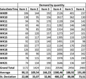
The company orders the items from supplier as produced and there is no need for extra manufacturing process. We assume that products have zero lead time and entire order quantity is delivered at the same time. Table 1 shows products’ actual demand as weekly basis.
TABLE I. WEEKLY DEMAND BY QUANTITY
We randomly have chosen demand data between week 9 and week 21, which we believe is the peak season for consumer electronic market. According to the demand data, we assume that demand is stationary and the forecast errors are normally distributed as in Eynan and Kropp [9]. This assumption can be based on some reasons. In many cases, the normal distribution provides a better fit to data than most other distributions. Moreover, since the planning time horizon is infinite, forecast errors are added together, so normal distribution can be expected through the Central Limit Theorem. Finally, the normal distribution leads to analytically tractable results [9].
The experimentation is carried out via spreadsheet and RAND algorithms for both deterministic and stochastic cases. At first, we run RAND and Spreadsheet algorithms for deterministic case. After that, calculation for stochastic structure is implemented through using standard deviation. We compare the results for the proposed stochastic spreadsheet algorithm with well known heuristic RAND for stochastic cases. In order to calculate the results, we used
SalesDateTime Item 1 Item 2 Item 3 Item 4 Item 5 Item 6
WK09 106 144 192 2126 401 237
WK10 138 95 156 2617 362 130
WK11 94 76 170 1139 194 142
WK12 65 46 211 1282 146 148
WK13 78 85 228 1314 166 262
WK14 69 120 157 1273 147 101
WK15 65 117 144 1395 133 129
WK16 92 123 140 1491 139 98
WK17 102 177 122 1134 170 250
WK18 126 102 131 1055 182 227
WK19 85 90 135 2096 154 342
WK20 78 115 185 1978 126 230
WK21 74 134 190 1646 136 187
Grand Total 1172 1424 2161 20546 2456 2483
Average 90,15 109,54 166,23 1580,46 188,92 191,00
St. Deviation 22,88 33,07 32,86 480,23 88,08 73,51
MATLAB and we coded for RAND [10], spreadsheet [11], stochastic RAND [9] and finally proposed spreadsheet algorithm under stochastic demand environments.
In order to compare our results with Eynan and Kropp [9], we used same cost data for minor, major and holding cost. We took the average demand according to our real world data and standard deviation as sigma in the formulas. Service level is taken as 1.64. The data is presented in Table 2:
TABLE II. DATA FOR THE NUMERICAL EXPERIMENT
As indicated before, we tested four algorithms, and the deterministic case of the problem is calculated through using average demand. In the RAND algorithm, m is taken as 5. In the spreadsheet algorithm, quotient is taken as 1.4. For the stochastic case of the problem, standard deviation of each item is considered. The results of algorithms are presented in Table 3.
TABLE III. THE RESULTS FOR SPREADSHEET AND RAND ALGORITHMS
According to Table 3, spreadsheet and RAND methods for deterministic case give same result in terms of total cost, whereas in stochastic case our proposed spreadsheet algorithm outperformed stochastic RAND algorithm. The proposed spreadsheet algorithm gives total cost as 374.82, whereas stochastic RAND algorithm’s is 375.14.
TABLE IV. WEEKLY DEMAND FOR WEEK 22–34 AS FUTURE DATA
Deterministic algorithms give lower cost than stochastic algorithms. However, taking average demand into account
by itself may give incorrect strategy in terms of customer service rates. Generally, retailers ignore the variation and prefer to use deterministic algorithm. Therefore, we calculated customer service level both deterministic spreadsheet and proposed stochastic spreadsheet algorithm. In order to test customer service rate, we used the data between week 22 and week 34 as future demand which follows our previous test data.
In order to test customer service rate for both models, we calculated the real demand in the replenishment interval for each item and order quantity in each replenishment cycle. Since backordering does not exist in our model, the assumption is that if demand is higher than on hand stock, it is considered as lost sale. Replenishment quantity is obtained according to the data between week 9 and week 21, tested on week 22 and week 34 to calculate customer service rate.
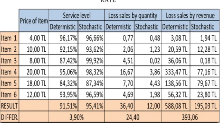
The summary of calculation is presented in Table 5. For customer service rate, deterministic strategy gives 91.51%, whereas with the stochastic strategy 95.41% of customer’s demand can be fulfilled. Moreover, loss of revenue can be calculated by each item’s average lost quantity in a replenishment interval multiplied with its price, since backordering is not allowed in the system. Thus, loss revenue is 588.08 TL in the deterministic method, compared to 195.03 TL for stochastic method. This calculation can be interpreted as the difference 393.06 TL will be the charge of unmet customer demand, whereas total cost difference is 181.83 TL by using stochastic replenishment strategy.
TABLE V. RESULTS OF THE CALCULATION FOR CUSTOMER SERVICE RATE
After all the calculations, we can draw some conclusions for our real-world data set. Stochastic spreadsheet algorithm outweigh stochastic RAND algorithm in terms of total cost charges. Therefore, it is logical to use our proposed algorithm as an effective replenishment strategy. Moreover, customer service rate increased from 91.51% to 95.41% through using stochastic replenishment strategy.
VI. CONCLUSION
In this paper, we presented a new adaptation of spreadsheet heuristic for stochastic environments. The simplicity of application of spreadsheet method and its efficiency enabled us to consider its modified version for the joint replenishment problem under stochastic version. We offered to consider not only average demand value, but also variability in demand function. Since consumers’ preferences are getting harder to predict, the importance of
Item 1 Item 2 Item 3 Item 4 Item 5 Item 6 Average Demand 90,15 109,54 166,23 1580,46 188,92 191,00
Standart Deviation 22,88 33,07 32,86 480,23 88,08 73,51
Holding Cost 0,4 1,0 0,8 0,2 0,8 0,2
Minor repl. Cost 1,8 2,0 1,2 3,2 3,1 2,7
Major repl. Cost 10
Service Level 1,64
Spreadsheet RAND Proposed Spreadsheet Stochastic RAND
TC 192,99 192,99 374,82 375,14
T 0,2251 0,2347 0,1649 0,1598
Deterministic Stochastic
SalesDateTime Item 1 Item 2 Item 3 Item 4 Item 5 Item 6
WK22 125 117 168 1463 318 203
WK23 88 124 86 1916 335 246
WK24 49 107 101 1670 201 187
WK25 139 107 83 1641 135 203
WK26 73 122 118 1785 286 194
WK27 77 172 127 1863 176 177
WK28 120 87 143 1444 146 196
WK29 72 132 221 1135 117 192
WK30 34 71 276 1183 141 133
WK31 26 147 288 1057 335 128
WK32 147 107 113 1447 156 76
WK33 93 99 135 1320 255 135
WK34 104 129 220 1312 197 256
Grand Total 1147 1521 2079 19236 2798 2326
Average 88,23 117,00 159,92 1479,69 215,23 178,92 St. Deviation 38,34 25,83 69,57 279,06 80,53 49,65
Demand by quantity
Determistic Stochastic Determistic Stochastic Determistic Stochastic Item 1 4,00 TL 96,17% 96,66% 0,77 0,48 3,08 TL 1,94 TL Item 2 10,00 TL 92,15% 93,62% 2,06 1,23 20,59 TL 12,28 TL Item 3 8,00 TL 87,42% 99,92% 4,51 0,02 36,06 TL 0,18 TL Item 4 20,00 TL 95,06% 98,32% 16,67 3,86 333,47 TL 77,16 TL Item 5 18,00 TL 84,32% 87,34% 7,70 4,43 138,56 TL 79,67 TL Item 6 12,00 TL 93,95% 96,59% 4,69 1,98 56,32 TL 23,80 TL
RESULT 91,51% 95,41% 36,40 12,00 588,08 TL 195,03 TL
DIFFER.
Price of item Loss sales by quantity Loss sales by revenue
3,90% 24,40 393,06
variation is higher than before. For this reason, we thought that if variation in demand is taken into account, it would give more accurate results for retailers in supply chain.
In order to test and compare the algorithms, the real world data was constructed and run to find out how effective the proposed algorithm is. The numerical data belongs to a world-wide known consumer electronic company. Because of the short life cycles and high obsolescence of technology products, accurate replenishment policy was highly required in this case. The uncertainty in demand can lead to the inventory’s accumulation and also shortages in terms of availability. In order to balance the trade-off between high inventory level and shortage, an effective replenishment strategy was essential for our business problem.
We compared the effectiveness of our proposed algorithm with well a known RAND heuristic for joint replenishment problems. In the deterministic case of the problem, both algorithms gave same result, whereas proposed spreadsheet algorithm outperformed RAND algorithm for stochastic case. We utilized MATLAB for coding algorithms. We also highlighted the importance of using stochastic strategy with a calculation over deterministic strategy. The costumer service rate was computed for deterministic and stochastic strategies. Proposed stochastic strategy gives higher customer service level which means lower unmet customer demand. In conclusion, proposed stochastic spreadsheet algorithm performs well for the real world data and is appropriate for the company’s replenishment strategy.
The proposed algorithm could be extended in several directions. For instance, backordering cost could be implemented to the algorithm. In this way, shortage cost could also be considered in addition to the holding costs and the replenishment costs. Furthermore, the concept developed could be applied under direct grouping strategy. Products could be partitioned into predetermined number of sets that are jointly replenished. We believe that future modifications may increase performance.
ACKNOWLEDGMENT
This research has been financially supported by Galatasaray University Research Fund.
REFERENCES
[1] Aksoy, Y., and Erenguc, S. S., “Multi-item inventory models with coordinated replenishments: a survey.” International Journal of Operations and Production Management, 8, 63- 73, (1987).
[2] Brown, R.G., “Decision Rules for Inventory Management.” Holt, Rinehart and Winston, New York, NY. 48, (1967)
[3] Goyal, S.K. “Determination of optimum packaging frequency of items jointly-replenished.” Management Science, 21,436- 443, (1974) [4] Silver, E.A., “A simple method of determining order quantites In joint
replenishments under deterministic demand”. Management Science, 22, 1351-1361, (1976)
[5] Goyal, S.K. and Belton, A.S. “On a simple method of determining order quantities in joint replenishments under deterministic demand.” Management Science, 25, 604, (1979)
[6] Kaspi, M. and Rosenblatt, M.J. “An improvement of Silver's algorithm for the joint replenishment problem.” IIE Transactions. 15, 264-267, (1983)
[7] Atkins, D.R. and lyogun, P.O. “A heuristic with lower bound performance guarantee for the multi-product dynamic lot size problem.” IIE Transactions, 20, 369-373, (1988)
[8] Silver, E.A. and Meal, H.C. “A heuristic for selecting lot size requirements for the case of a deterministic time-varying demand rate and discrete opportunities for replenishment.” Production and Inventory Management. 14. 64-74, (1973)
[9] Eynan, A. and Kropp D.H. “Periodic review and joint replenishment in stochastic demand environments.” IIE Transactions. 30:11, 1025-1033, (1998).
[10] Kaspi, M. and Rosenblatt, M.J. “On the economic ordering quantity for jointly replenished items.” International Journal of Production Research, 29:1, 107-114, (1991)
[11] Nilsson, A., Segerstedt, A., Sluis, E. “A new iterative heuristic to solve the joint replenishment problem using a spreadsheet technique.” Int. J. Production Economics 108, 399–405, (2007).
[12] Balintfy, J.L “On a basic class of multi-items inventory problems” Management Science, 10 (2), pp. 287–297, (1964).
[13] Silver, E.A, “A control system for coordinated inventory replenishment,” International Journal of Production Research, 12 pp. 647–670, (1974).
[14] Federgruen, A., Groenevelt H., Tijms H.C., “Coordinated replenishments in a multi-item inventory system with compound Poisson demands,” Management Science, 30, pp. 344–357, (1984), [15] Zheng, Y.S, “Optimal control policy for stochastic inventory systems
with Markovian discount opportunities,” Operations Research, 42 (4), pp. 721–738, (1994).
[16] Melchiors, P., “Calculating can-order policies for the joint replenishment problem by the compensation approach,” European Journal of Operational Research Volume 141, Issue 3, Pages 587– 595, (2002).
[17] Evans, R.V. “Inventory control of a multiproduct system with a limited production resource. “Naval Research Logistics Quarterly, 14, 173–184, (1967).
[18] Florian, M. and Klein, M. “Deterministic production planning with concave costs and capacity constraints.” Management Science, 18, 12–20, (1971).
[19] De Kok, A., Tijms, H. and Van der Duyn Schouten, F. “Approximations for the single-product production-inventory problem with compound Poisson demand and service level constraints.” Advances in Applied Probability. 16, 378–402, . (1984)
[20] Choi,J. Cao J., Romeijn, H. E., Geunes, J. and Bai, A.S, “Stochastic multi-item inventory model with unequal replenishment intervals and limited warehouse capacity.” IIE Transactions 37, 1129–1141, (2005). [21] Nahmias, S. “Production and Operation Analysis”, Irwin Homewood,
ΙΙΙ. (1993).
[22] Olsen A. L., “An evolutionary algorithm to solve the joint replenishment problem using direct grouping.” Computers & Industrial Engineering 48, 223–235, (2005).
[23] Hsu, S., “Optimal joint replenishment decisions for a central factory with multiple satellite factories.” Expert Systems with Applications 36, 2494–2502, (2009).