OSD
11, 839–893, 2014Phytoplankton and vertical mixing
L. Hahn-Woernle et al.
Title Page
Abstract Introduction
Conclusions References
Tables Figures
◭ ◮
◭ ◮
Back Close
Full Screen / Esc
Printer-friendly Version Interactive Discussion
Discussion
P
a
per
|
D
iscussion
P
a
per
|
Discussion
P
a
per
|
Discuss
ion
P
a
per
|
Ocean Sci. Discuss., 11, 839–893, 2014 www.ocean-sci-discuss.net/11/839/2014/ doi:10.5194/osd-11-839-2014
© Author(s) 2014. CC Attribution 3.0 License.
Open Access
Ocean Science
Discussions
This discussion paper is/has been under review for the journal Ocean Science (OS). Please refer to the corresponding final paper in OS if available.
Sensitivity of phytoplankton distributions
to vertical mixing along a North Atlantic
transect
L. Hahn-Woernle1, H. A. Dijkstra1, and H. J. Van der Woerd2
1
Institute for Marine and Atmospheric Research Utrecht (IMAU), Dept. of Physics and Astronomy, Utrecht University, P.O. Box 80.005, 3508 TA Utrecht, the Netherlands
2
Institute for Environmental Studies (IVM), Free University of Amsterdam, the Netherlands
Received: 31 January 2014 – Accepted: 20 February 2014 – Published: 14 March 2014 Correspondence to: L. Hahn-Woernle ([email protected])
OSD
11, 839–893, 2014Phytoplankton and vertical mixing
L. Hahn-Woernle et al.
Title Page
Abstract Introduction
Conclusions References
Tables Figures
◭ ◮
◭ ◮
Back Close
Full Screen / Esc
Printer-friendly Version Interactive Discussion
Discussion
P
a
per
|
D
iscussion
P
a
per
|
Discussion
P
a
per
|
Discuss
ion
P
a
per
Abstract
Using in situ data of upper ocean vertical mixing profiles along a transect in the North Atlantic and an idealised phytoplankton growth model (PGM), we study the sensitiv-ity of the surface phytoplankton concentration to vertical mixing distributions. Optical parameters in the PGM are calibrated with observations of light attenuation. The
cali-5
bration of the biological parameters in the PGM is carried out at three different referent stations with observed vertical profiles of chlorophylla(Chla) and nutrient concentra-tion. Vertical mixing profiles at all other stations are next used at the reference stations to study the sensitivity of modelled phytoplankton distributions to vertical mixing. We find that shifts in vertical mixing are able to induce a transition from an upper
chloro-10
phyll maximum to a deep one and vice-versa. Furthermore, a clear correlation between the surface phytoplankton concentration and the mixing induced nutrient flux is found in nutrient limited regions. This may open up the possibility to extract characteristics of vertical mixing from satellite ocean colour data using data-assimilation methods.
1 Introduction
15
Thanks to the long-term in situ and satellite observations, the study of the plankton variability on time scales longer than seasonal has come within reach. On interannual-to-decadal time scales, changes in chlorophylla(Chla) concentrations can be well cor-related (Martinez et al., 2009) to variations in climate indices such as the North Atlantic Oscillation. Based on a century long database of in situ Chlaand ocean transparency
20
measurements, long-term trends in Chla were presented in Boyce et al. (2010). Al-though the results are under debate, it is clear that long-term trends in Chlaare non-uniform over the globe and well correlated to the increase in sea surface temperature (SST). For the North Atlantic (north of 20◦N), Wernand et al. (2013) found an average rate of increase of about 0.0071 mg (m3yr)−1 over the last century. On a shorter time
OSD
11, 839–893, 2014Phytoplankton and vertical mixing
L. Hahn-Woernle et al.
Title Page
Abstract Introduction
Conclusions References
Tables Figures
◭ ◮
◭ ◮
Back Close
Full Screen / Esc
Printer-friendly Version Interactive Discussion
Discussion
P
a
per
|
D
iscussion
P
a
per
|
Discussion
P
a
per
|
Discuss
ion
P
a
per
|
scale (decades), however, much larger local variations are observed (Antoine et al., 2005).
Although the precise details of a phytoplankton bloom are still not clarified, most of the theories consider vertical mixing as a key factor in its onset (Behrenfeld et al., 2006). During winter, deep mixing brings nutrients into the euphotic layer but light is
5
limited. In spring, the shallowing of the mixed layer allows the phytoplankton to spend more time exposed to light. The latter enhances growth and leads to an upper chloro-phyll maximum (UCM) when enough nutrients are available (Behrenfeld, 2010; Lozier et al., 2011). Since photosynthetically active radiation (PAR) is absorbed at the surface, less radiation penetrates the water column, which has a strong impact on the growth
10
below the mixed layer. As soon as the necessary nutrients (e.g. phosphorus and nitro-gen) are depleted, the phytoplankton concentration in the mixed layer decreases giving the phytoplankton below the mixed layer the possibility to grow. In this case most of the phytoplankton cells are found below the mixed layer forming a so-called deep chloro-phyll maximum (DCM). A DCM is the most dominant appearance of phytoplankton in
15
strongly stratified regions such as the sub-tropical North Atlantic.
Qualitative mechanisms aiming to explain the relation between SST and Chla con-centrations have, for example, been suggested by Doney (2006). In areas where phy-toplankton is nutrient limited, e.g. in the mid-latitude Atlantic, an increase in SST will inhibit vertical mixing and lead to stratification. In a warming ocean the transport of
20
nutrients into the upper ocean is hence expected to decrease. In areas where the phy-toplankton is light limited, such as in the northern North Atlantic, an SST increase will reduce the depth of the mixed layer and hence one would expect an increase in phy-toplankton. The fact that this trend is not observed in high-latitude regions according to data in Boyce et al. (2010) indicates that vertical mixing processes are not solely
25
OSD
11, 839–893, 2014Phytoplankton and vertical mixing
L. Hahn-Woernle et al.
Title Page
Abstract Introduction
Conclusions References
Tables Figures
◭ ◮
◭ ◮
Back Close
Full Screen / Esc
Printer-friendly Version Interactive Discussion
Discussion
P
a
per
|
D
iscussion
P
a
per
|
Discussion
P
a
per
|
Discuss
ion
P
a
per
heat and salt due to ocean currents, and in particular by the presence of meso-scale eddies (McGillicuddy et al., 2007).
At any particular location in the open ocean, the vertical profile of the mixing co-efficientKT [m
2
s−1] (for heat and salt) is determined by the background stratification (or buoyancy frequencyN), the turbulent kinetic energy dissipation rateε[m2s−3] and
5
a mixing efficiency (Jurado et al., 2012b). Over the last decade, microstructure turbu-lence measurements of the upper ocean have been carried out along a few sections in the Atlantic Ocean, see Roget et al. (2006) for an overview. Using a microstructure profiler, the distribution ofKT along a south to north transect in the eastern North At-lantic during the STRATIPHYT-I cruise in July–August 2009 and the STRATIPHYT-II
10
cruise in April–May 2011 was determined (Jurado et al., 2012b, a). Satellite ocean colour observations (MODIS-AQUA) of August 2009 indicate a meridional gradient in Chlaat this time of the year. The profiles ofKT along this section clearly indicate high values in the upper mixed layer and a decrease near the base of the mixed layer. At some locations the averaged station profiles of KT slightly increase below the mixed 15
layer before background values of 10−5–10−4m2s−1 are approached at about 100 m depth. In spring 2011 satellite ocean colour observations are characterised by a high concentration around 45◦N and decreasing Chl a concentrations north and south of this. In situ vertical mixing profiles ofKT indicate that the water column is stratified up to about this latitude. Further north the water column is more homogeneously mixed
20
down to 100 m depth (Jurado et al., 2012b, a).
The effect of vertical mixing on phytoplankton distributions can be studied using ocean-phytoplankton models. These models, however, contain a number of uncertain parameters both in the turbulence model and in the plankton model. Usually, the pa-rameter values are “tuned” to observations at one particular well-observed location and
25
OSD
11, 839–893, 2014Phytoplankton and vertical mixing
L. Hahn-Woernle et al.
Title Page
Abstract Introduction
Conclusions References
Tables Figures
◭ ◮
◭ ◮
Back Close
Full Screen / Esc
Printer-friendly Version Interactive Discussion
Discussion
P
a
per
|
D
iscussion
P
a
per
|
Discussion
P
a
per
|
Discuss
ion
P
a
per
|
This work is motivated by the availability of an observed integral picture (forcing, mixing, nutrients, phytoplankton, optical properties) over the eastern Atlantic transect during Summer 2009 and Spring 2011 from the STRATIPHYT cruises. Using ocean-plankton models and data-assimilation methods we eventually aim to tackle an ambi-tious inverse problem: provided satellite derived ocean colour data and the
meteoro-5
logical surface forcing, can we estimate the vertical mixing coefficientKT in the upper ocean? As a first step, we study here the sensitivity of the surface phytoplankton con-centration to the profile of the vertical mixing coefficient. Thereto we use an idealised phytoplankton growth model (Huisman and Sommeijer, 2002; Ryabov et al., 2010) to-gether with the measuredKT profiles during the two cruises.
10
The paper is structured as follows. In Sect. 2, the relevant satellite data and the mea-surements of the STRATIPHYT cruises are presented. Next, in Sect. 3, the idealised phytoplankton growth model is presented and its calibration (e.g. parameter tuning) is discussed in Sect. 4. The main analysis of the sensitivity of the equilibrium phytoplank-ton distributions to the vertical mixing profiles appears in Sect. 5. Finally, in Sect. 6 the
15
results are discussed and the conclusions are formulated.
2 Data
For the analysis presented in this paper, we use both satellite colour data as well as in situ data measured during the STRATIPHYT cruises. Additional information on this data can be obtained from http://oceancolor.gsfc.nasa.gov and http://projects.nioz.nl/
20
stratiphyt, respectively.
2.1 Satellite data
During the past decades the range of applications for satellite data and their re-liability has improved significantly. An important application is the measurement of Chla surface concentration which can be used as a measure for the phytoplankton
OSD
11, 839–893, 2014Phytoplankton and vertical mixing
L. Hahn-Woernle et al.
Title Page
Abstract Introduction
Conclusions References
Tables Figures
◭ ◮
◭ ◮
Back Close
Full Screen / Esc
Printer-friendly Version Interactive Discussion
Discussion
P
a
per
|
D
iscussion
P
a
per
|
Discussion
P
a
per
|
Discuss
ion
P
a
per
concentration close to the ocean surface. The data is based on the reflectance of blue and green wavelengths and can therefore only be obtained for the first meters of the water column. Figure 1b shows 1◦×1◦ box averaged and monthly mean values of the Chla surface concentration recorded by the MODIS on the Aqua satellite. To retrieve the Chla concentrations from MODIS Aqua ocean colour data, the OC3 M algorithm
5
(O’Reilly et al., 2000) is used. The data is plotted along the ship track in the North At-lantic during the STRATIPHYT cruises (shown in Fig. 1a) over the years 2009 to 2011. Black data points correspond to gaps in the data, e.g. due to high cloud coverage or the lack of sunlight. PAR was measured during the CTD casts of both STRATIPHYT cruises. Since these are very instantaneous measurements, which vary strongly not
10
only with the daily cycle of the sun but also due to cloud coverage, daily mean Aqua MODIS Photosynthetically Available Radiation data was used for the PGM.
2.2 In situ data
During the two STRATIPHYT cruises in summer 2009 and spring 2011 the ship stopped multiple hours per latitudinal station which allowed the scientists to measure
15
several depth profiles per station. Though these measurements give only snapshots into the vertical structure of the North Atlantic, there is evidence (Jurado et al., 2012b) that they are a good representation of the seasonal characteristics. We will therefore refer to the data sets of the 2009 and 2011 cruises as summer data and spring data, respectively.
20
The obtained temperature microstructure measurements were used to derive depth profiles for the vertical mixing coefficient (KT [m2s−1]) according to the Osborn (1972) model.KT was computed from the temperature variance dissipation rate, χT [◦C s−1], according to
χT=6DT
∂T′
∂z
2
; KT =χT 2
∂T ∂z
!−2
, (1)
OSD
11, 839–893, 2014Phytoplankton and vertical mixing
L. Hahn-Woernle et al.
Title Page
Abstract Introduction
Conclusions References
Tables Figures
◭ ◮
◭ ◮
Back Close
Full Screen / Esc
Printer-friendly Version Interactive Discussion
Discussion
P
a
per
|
D
iscussion
P
a
per
|
Discussion
P
a
per
|
Discuss
ion
P
a
per
|
where DT is the molecular diffusivity of heat (≈1.4×10⁻⁷m2s−1) and ∂T /∂z and
∂T′/∂z are the mean and fluctuation part of the temperature gradient (for details see Jurado et al., 2012b).
In Fig. 2 the station-mean, smoothed and interpolated profiles forKT are shown for both cruises (Jurado et al., 2012a, b). Here, the profiles are smoothed over windows of
5
5 m depth to guarantee the compatibility with the numerical scheme used in the phyto-plankton model, as will be explained below. The mixed layer depth (MLD, dashed line in Fig. 2) is defined as the depth at which the temperature difference with respect to the surface is 0.5◦C (Levitus et al., 2000). In spring, the MLD ranges between 20 m and 60 m for stratified stations up to 46◦N. Further north, the water column is nearly
10
homogeneously mixed. In summer, the profiles of the mixing coefficient show strati-fied characteristics for all stations with maximum values of the MLD around 45 m. The strength of the vertical mixing and its vertical properties change both seasonally as well as latitudinally.
In situ measurements of phosphorus and nitrogen show that there is a gradient in
15
the nutricline between south and north (van de Poll et al., 2013). For simplicity we generalize the overall concentration of phosphorus, nitrogen, and nitrate as nutrients. According to the measured data, the water column provides sufficient nutrients for the phytoplankton to grow close to the surface in the northern stations, a so-called mesotrophic state. At stations further south the surface layer is practically depleted of
20
nutrients and therefore oligotrophic. The transition between the oligotrophic and the mesotrophic stations lies at about 40◦N during the spring cruise and at about 45◦N during the summer cruise. The comparison with the Chlaprofiles in Fig. 3 shows that these are also the latitudes of transition from an deep chlorophyll maximum (DCM) to an upper chlorophyll maximum (UCM).
25
OSD
11, 839–893, 2014Phytoplankton and vertical mixing
L. Hahn-Woernle et al.
Title Page
Abstract Introduction
Conclusions References
Tables Figures
◭ ◮
◭ ◮
Back Close
Full Screen / Esc
Printer-friendly Version Interactive Discussion
Discussion
P
a
per
|
D
iscussion
P
a
per
|
Discussion
P
a
per
|
Discuss
ion
P
a
per
on the fluorescence in units of the Chelsea Aqua 3 Chlaconcentration (g/l) and were measured down to depths of 200 m. The conversion from Chl a to cells is based on a combined conversion factor of Ryabov et al. (2010) and Omta et al. (2009) (see Sect. 4.1). Well-mixed stations, as in the north during spring, show a homogeneous distribution of phytoplankton cells over the first 100 m depth. Stratification forces the
5
phytoplankton to grow either within the mixed layer and to form an UCM, or to grow below the mixed layer in a DCM.
Figure 3 as well as the MODIS Aqua data in Fig. 1b show that the transition from the UCM to the DCM happens later in the year and has a shorter duration the further north one observes the surface Chlaconcentration. At latitudes north of 45◦N surface
10
concentrations remain relatively high throughout the entire light season, while regions south of 45◦N exhibit very low Chlaconcentrations during summer. Irrespective of the latitude, locally and temporally restricted surface Chlamaxima are also seen indepen-dent of the stratification cycle, e.g. in MODIS Aqua data, and these maxima have been suggested to be connected to ocean eddies (Mahadevan et al., 2012).
15
3 Phytoplankton growth model
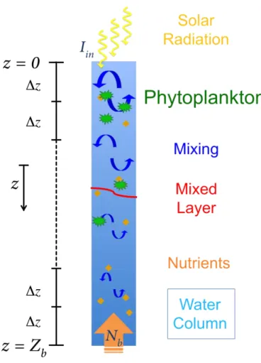
The phytoplankton growth model (PGM) is based on the advection-reaction-diffusion models by Huisman and Sommeijer (2002) and Ryabov et al. (2010). Figure 4 provides a sketch of the basic model setup and the processes controlling growth and phytoplank-ton distribution in the model. Phytoplankphytoplank-ton cells need nutrients and light to grow and
20
their number is reduced at a constant rate representing sedimentation and grazing. Sunlight penetrates the water at the surface (yellow arrows) and its intensity decreases with depth due to the background attenuation of sea water and absorption by phy-toplankton cells. Vertical mixing (blue arrows) is represented as a depth-dependent diffusion coefficient and it distributes nutrients (orange diamonds) and phytoplankton
25
OSD
11, 839–893, 2014Phytoplankton and vertical mixing
L. Hahn-Woernle et al.
Title Page
Abstract Introduction
Conclusions References
Tables Figures
◭ ◮
◭ ◮
Back Close
Full Screen / Esc
Printer-friendly Version Interactive Discussion
Discussion
P
a
per
|
D
iscussion
P
a
per
|
Discussion
P
a
per
|
Discuss
ion
P
a
per
|
3.1 Governing equations
In a water column of depthZbthe density of phytoplankton cells at timet >0 and
verti-cal positionz∈[0,Zb], where z=0 indicates the surface andz is positive downwards,
is denoted byP(z,t) (Fig. 4). The two controlling factors for phytoplankton growth are the concentration of nutrientsN(z,t) and the intensity of lightI(z,t). The coupling of
nu-5
trient and phytoplankton dynamics is described by the following two equations (Ryabov et al., 2010):
∂P
∂t =growth−loss−sinking+vertical mixing
=µ(N,I)P−mP−v∂P ∂z +
∂ ∂z
KT(z)
∂P ∂z
,
(2)
∂N
∂t =−uptake+recycling+vertical mixing
=−αµ(N,I)P +εαmP + ∂
∂z
KT(z)
∂N ∂z
,
(3)
10
whereµ(N,I) describes the local growth. Furthermore,mis the mortality,vis the sink-ing velocity, KT(z) is the depth dependent vertical mixing coefficient,α is the nutrient
content of a phytoplankton cell andεis the nutrient recycling coefficient.
No flux conditions are assumed at the surfacez=0 for both the phytoplankton con-centration and the nutrient concon-centration. At the bottom boundary,z=Zb, the nutrient 15
density is prescribed as constant valueNb, which represents a infinite source of
nutri-ents in the deep ocean. The magnitude of this source is latitude dependent and based on measurements as discussed below and shown in Table 3. The initial phytoplankton concentration P is based on the measured profiles. Since Zb lies well below the
eu-photic layer, the lower boundary condition for the phytoplankton concentration is kept
20
OSD
11, 839–893, 2014Phytoplankton and vertical mixing
L. Hahn-Woernle et al.
Title Page
Abstract Introduction
Conclusions References
Tables Figures
◭ ◮
◭ ◮
Back Close
Full Screen / Esc
Printer-friendly Version Interactive Discussion
Discussion
P
a
per
|
D
iscussion
P
a
per
|
Discussion
P
a
per
|
Discuss
ion
P
a
per
Growth and loss coupleP toN via the uptake of nutrients and the partial recycling of dead phytoplankton cells. The growth rateµ(N,I) has a strong local dependence on the available resources and is written as:
µ(N,I)=µmax min
N
HN+N
, I
HI+I
, (4)
5
whereµmaxis the maximum growth rate of phytoplankton andHNandHI are the
half-saturation constants of nutrient limited and of light limited growth, respectively. For example, the value ofHNis relatively low for species which are well adapted to nutrient
limited regimes.
The intensity of light as a function of vertical position z and time t is given by the
10
Beer–Lambert’s equation
I(z,t)=Iin exp
−Kbgz−k
z
Z
0
P(ξ,t)d ξ
, (5)
where Iin denotes the intensity of the incoming light at the surface of the water
col-umn. The intensity of light within the water column decreases with depth due to a
con-15
stant background attenuation represented byKbg[m
−1
]. Additionally, each phytoplank-ton cell absorbs photosynthetic active radiation which leads to a shading effect on the whole water column below the cell; this effect is represented by the term involvingk
[m2cell−1]. SinceI(zi,t) is dependent on phytoplankton concentrations at depthsz≤zi,
the PGM is a non-local model.
20
3.2 Numerical implementation
In the PGM, vertical mixing is defined by a prescribed vertical mixing profile KT(z)
and here we make use of the measured vertical mixing profiles of KT as presented in Sect. 2. As the bottom boundary of the modelZb=200 m, these profiles were
OSD
11, 839–893, 2014Phytoplankton and vertical mixing
L. Hahn-Woernle et al.
Title Page
Abstract Introduction
Conclusions References
Tables Figures
◭ ◮
◭ ◮
Back Close
Full Screen / Esc
Printer-friendly Version Interactive Discussion
Discussion
P
a
per
|
D
iscussion
P
a
per
|
Discussion
P
a
per
|
Discuss
ion
P
a
per
|
data points within the vertical profile were linearly interpolated from the nearest avail-able data points. Finally the profiles were smoothed over windows of 5 m depth. This is done to guarantee the compatibility with the diffusion scheme used in the phytoplank-ton model.
In situ measurements of PAR at the water surface vary strongly and on time scales
5
of hours and less. ThereforeIinis initialised with the daily mean Aqua MODIS PAR data
on the date and at the location of the according station. Since we study steady state situations,Iin is kept constant during each model run. The initial nutrient concentration
is assigned to the in situ profiles by van de Poll et al. (2013). While the vertical profile is changing according to Eq. (3), the bottom concentrationNbis kept constant to fulfill
10
the boundary conditions. This value changes with latitude and season.
To solve the differential equations Eqs. (2) and (3) the NAG D02EJF routine (see for more details http://www.nag.co.uk) is used with a time step of 24 h. A grid spacing ∆z=0.25 m has to be applied to obtain sufficiently accurate solutions due to the strong vertical variation over some vertical mixing profiles. In all simulations, the model is run
15
for a time interval of 500 days. The PGM adjusts to the environmental conditions within the first 50 to 100 days of the simulation. Thereafter variations in the system state hap-pen mainly on time scales of the vertical mixing and the time to reach an equilibrium state can range from 100–1000 days. The in situ measurements did not only show strong seasonal variations but also moderate diurnal changes (not included here).
Ver-20
tical mixing and therefore the environmental conditions on phytoplankton growth are therefore unlikely to maintain their major properties over periods longer than a few months. Our choice of 500 days is therefore a period which is long enough to equili-brate the system and which still represents a fairly realistic time frame of the relevant physical and biological processes.
25
OSD
11, 839–893, 2014Phytoplankton and vertical mixing
L. Hahn-Woernle et al.
Title Page
Abstract Introduction
Conclusions References
Tables Figures
◭ ◮
◭ ◮
Back Close
Full Screen / Esc
Printer-friendly Version Interactive Discussion
Discussion
P
a
per
|
D
iscussion
P
a
per
|
Discussion
P
a
per
|
Discuss
ion
P
a
per
(based on a generalized Fermi function, see Ryabov et al., 2010, for more details). The results in Huisman et al. (2006) show that the state of the phytoplankton profile is strongly dependent on the strength of the vertical mixing. The combination of light and nutrient limitation, sinking and low vertical mixing eventually leads to an unstable steady state and the amount of biomass undergoes a transition to an oscillatory state. Ryabov
5
et al. (2010) studied the effect of stratification on the model state and forced the system into DCM and UCM states by changing the strength of the vertical mixing. We have performed similar studies with our version of the PGM and the results of the Ryabov et al. (2010) work could successfully be reproduced. The PGM is therefore capable to simulate different phytoplankton growth states dependent on the characteristics of the
10
applied vertical mixing.
4 Calibration of the model
In the PGM various physical, optical, biological, and chemical parameters appear, as given in Table 1. The measurements allow us to calibrate most of these parameters. Optical parameters like Kbg and k can be determined by combining Eq. (5) to the 15
measured light profile (see Appendix for a description of the method). In Sect. 4.1 the calibration of the values of these coefficients is presented. The values of the bio-logical parameters affect the modelled growth behaviour of the phytoplankton. Many experiments and measurements are made to determine for example the growth rate of individual phytoplankton species in a specific environment (Peters et al., 2006). Results
20
show that growth rates do not only vary between species but also due to environmental changes. The biological data of the STRATIPHYT project shows that the Chlaprofiles originate from compositions of different phytoplankton species (van de Poll et al., 2013). Simulating the phytoplankton growth at STRATIPHYT stations by means of the PGM, in which growth is represented by a single species, requires calibration of the
biolog-25
OSD
11, 839–893, 2014Phytoplankton and vertical mixing
L. Hahn-Woernle et al.
Title Page
Abstract Introduction
Conclusions References
Tables Figures
◭ ◮
◭ ◮
Back Close
Full Screen / Esc
Printer-friendly Version Interactive Discussion
Discussion
P
a
per
|
D
iscussion
P
a
per
|
Discussion
P
a
per
|
Discuss
ion
P
a
per
|
andHN, respectively, are calibrated to the in situ measurements. The results of the two
calibration steps are discussed in Sect. 4.3.
4.1 Optical parametersk andKbg
As described above, fluorescence is a measure of Chl a in water while in the PGM, phytoplankton is represented in cell numbers. The ratio of Chl a per cell can vary
5
significantly depending on species and environmental conditions. Up to now there is no universal equation explaining this complex relation (Falkowski and Raven, 2007). Therefore a general ratio of 0.2×10⁹cells [µg Chla]−1is chosen for simplicity. This ra-tio is based on the cell:nutrient content rara-tio and the nutrient content : Chlaratio given by Ryabov et al. (2010) and Omta et al. (2009), respectively.
10
The transmittance of light in water can be affected by waves and a high concentration of small air bubbles at the surface as well as phytoplankton, sediments and dissolved organic material in the water column. It is beyond the scope of this work to quantify all these effects. Since surface effects are very localised and sediment concentrations are very low in open water they are both not taken into account in the analysis. Our
15
aim is rather to identify the characteristics of the light attenuation due to the two major contributions as represented byKbgandk in Eq. (5).
In Eq. (5) the dependence of the light intensity is given as an exponential function of depth. Figure A1 in the Appendix shows an example of a vertical CTD profile mea-suring fluorescence (green), surface irradiance (red), and corrected irradiance (blue,
20
logarithmic scaling). A very defined DCM is located at around 65 m depth. To deduce the values of Kbg and k from such measurement data the light profile is divided into
two sections: a Chl a free section at the bottom of the euphotic layer and a section of a high Chla concentration in the euphotic layer. The first section is used to deter-mine the attenuation only based onKbg. It is indicated by the blue interval in Fig. A1 25
OSD
11, 839–893, 2014Phytoplankton and vertical mixing
L. Hahn-Woernle et al.
Title Page
Abstract Introduction
Conclusions References
Tables Figures
◭ ◮
◭ ◮
Back Close
Full Screen / Esc
Printer-friendly Version Interactive Discussion
Discussion
P
a
per
|
D
iscussion
P
a
per
|
Discussion
P
a
per
|
Discuss
ion
P
a
per
the maximum concentration of phytoplankton. This section is referred to as the “green section” since it corresponds to the green shaded area in Fig. A1.
Making use of these localised properties of phytoplankton the quantities Kbg and
k are determined in two steps. First Kbg is calculated based on the blue section in
which the phytoplankton concentration has no influence (since it is approximately zero).
5
In the second step, k is determined over the green section with high phytoplankton concentration using theKbg value obtained at the first step. Details of the calculations are presented in the Appendix.
In the Fig. A3 the results ofKbgfor the STRATIPHYT spring and summer cruises can
be seen. For most stations multiple measurement profiles were available and the data
10
points shown are the mean values per station. The error bars in the graphs are based on the standard deviation between different profiles for one station. Stations defined by DCM states (south of the red dashed line in Fig. A3) show values for Kbg in the
range of 0.032 m−1. In stations with an UCM (north of the red dashed line and south of the green dashed line) the backscattering effect of particles could lead to an increased
15
absorption effect which affects the Kbg value since the backscattering is not implicitly
taken into account in our method (further details can be found in Siegel et al. (2005)). At northern latitudes of the spring cruise (north of the green dashed line) the Chlais homogeneously mixed over the entire measured depth. Therefore no blue section can be defined and henceKbg cannot be determined.
20
Applying the resulting meanKbgfound for the DCM states,kis determined based on
the green section of the Chlaprofiles; results are shown in Fig. A2. For the summer data, values ofkshow a mean of 5.9±1.9×10⁻¹⁰m2cell−1. The meank derived from the spring data is more than twice as high and to take both seasons into account a value ofk=10−9m2cell−1is chosen.
OSD
11, 839–893, 2014Phytoplankton and vertical mixing
L. Hahn-Woernle et al.
Title Page
Abstract Introduction
Conclusions References
Tables Figures
◭ ◮
◭ ◮
Back Close
Full Screen / Esc
Printer-friendly Version Interactive Discussion
Discussion
P
a
per
|
D
iscussion
P
a
per
|
Discussion
P
a
per
|
Discuss
ion
P
a
per
|
4.2 Growth parametersHI andHN
To calibrate the parametersHIandHNsuch that the PGM reproduces the main features of the measured Chl a profile, we assume that all measured profiles are in a steady state. The Least Squares Method (LSM) as implemented in the NAG E04FCF (an un-constrained optimization solver) is used. We choose two stations of the summer cruise
5
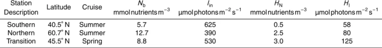
with different steady states: a DCM and a UCM. The DCM corresponds to measure-ments at the southern part of the track at 40.5◦N and the UCM to a more northern station at 60.7◦N. These stations are in the following referred to as the southern and northern station, respectively. Additionally, a third station of the spring cruise at 45.5◦N is chosen which shows a significant UCM in spring and a DCM in summer with still a
rel-10
ative high surface concentration of Chla(see Fig. 3). Because of this state change with the seasons we refer to it as the transition station.
The reference phytoplankton profiles are found in two different states: DCM and UCM. To define the residuals in the LSM, basic characteristics of the different phy-toplankton profiles have to be defined. In case of a DCM we choose the depth of the
15
DCM and its associated maximum phytoplankton concentration as the two major char-acteristics. In a UCM state, the phytoplankton cells are spread out over a wider depth range and hence the mean phytoplankton cell concentration and the mean nutrient concentration within the mixed layer are used. For each characteristicCi, the normal-ized difference between measuredCiobs and model determinedCimod value is used as
20
a residual in the LSM and the sum of squaresS is given by
S= v u u u t
X
i
1−C i mod
Ciobs
!2
OSD
11, 839–893, 2014Phytoplankton and vertical mixing
L. Hahn-Woernle et al.
Title Page
Abstract Introduction
Conclusions References
Tables Figures
◭ ◮
◭ ◮
Back Close
Full Screen / Esc
Printer-friendly Version Interactive Discussion
Discussion
P
a
per
|
D
iscussion
P
a
per
|
Discussion
P
a
per
|
Discuss
ion
P
a
per
4.2.1 The southern station
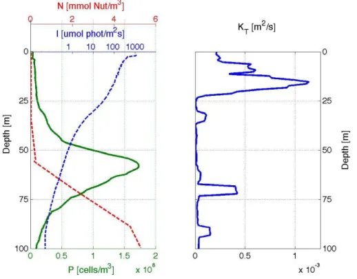
In Fig. 5 the biological, chemical, optical, and physical data profiles are shown for the southern station at (13.2◦W, 40.5◦N) on 23 July 2009. The green profile in the left panel gives the phytoplankton concentration with a maximum at around 60 m depth, clearly showing a DCM. The nutrient concentration (red dashed line) combines the measured
5
concentrations of phosphate (PO4), nitrogen dioxide (NO2), and nitrate (NO3) in one.
The main source of these nutrients is deeper, nutrient rich water (van de Poll et al., 2013) and it is clearly visible that the mixed layer is depleted of nutrients. Note that the light intensity profile (blue dashed line) is plotted with logarithmic scaling. Data is only available after a depth of 5 m. The light intensity decays exponentially and has very low
10
values at depths of the DCM and further below. The vertical turbulent mixing profile shows high values close to the surface decaying rapidly at a depth of approximately 25 m.
In Fig. 6a the interpolated result for the sum of squaresS, based on the depth and maximum value ofP at the DCM, is plotted vs.HIandHN. High values ofS are plotted 15
in red and resemble PGM results (based on a certain set ofHI and HN) that are very
different from the in situ profiles. Blue areas define sets of half-saturation constants for which the PGM result lies close to the observations. Note that the interpolation applied leads to a smoothing of the values ofS and is only chosen to show the complexity of the calibration ofHI andHN.
20
As can be seen in the center panel of Fig. 6b, the best match was achieved for the half-saturation constants HI=57 µmol photons m−2s−1 and HN= 0.54 mmol nutrients m−3. This figure does not only show that the system needs some time to adjust to the boundary conditions, but also demonstrates the effect of the half saturation constants on the properties of the phytoplankton profile. Increasing (HI,HN) 25
OSD
11, 839–893, 2014Phytoplankton and vertical mixing
L. Hahn-Woernle et al.
Title Page
Abstract Introduction
Conclusions References
Tables Figures
◭ ◮
◭ ◮
Back Close
Full Screen / Esc
Printer-friendly Version Interactive Discussion
Discussion
P
a
per
|
D
iscussion
P
a
per
|
Discussion
P
a
per
|
Discuss
ion
P
a
per
|
4.2.2 The northern station
In Fig. 7a the biological, chemical, optical, and physical data profiles are shown for the northern station at (19.3◦W, 60.7◦N) on 8 August 2009. The green line in the first panel on the left shows the phytoplankton concentration with a high cell concentration at the surface spreading over the whole mixed layer. The nutrient concentration (red dashed
5
line) combines again concentrations of phosphate (PO4), nitrogen dioxide (NO2) and
nitrate (NO3) in one. In contrast to the southern station, the mixed layer is not com-pletely depleted of nutrients though their concentrations are very low. Below the mixed layer the nutrient concentration increases quickly to its bottom value. The light intensity profile (blue dashed line) is again presented using a logarithmic scaling. The values
10
measured are almost half of what is measured at the southern station and the intensity decreases quickly over depth due to the high phytoplankton cell concentration within the mixed layer. The turbulent vertical mixing profile (right panel) differs from the one at the southern station since the strongest peak of mixing is located below the mixed layer.
15
The temporal evolution of the residuals of the LSM is shown in Fig. 7b as the plot of the nutrient residual (top), the sum of squares (center), and the phytoplankton resid-ual (bottom). All plots show that the model adjusts quickly and the absolute minimum was detected for HI=80 µmol photons m
−2
s−1 and HN=2.5 mmol nutrients m
−3
. The residual based on the mean phytoplankton concentration in the mixed layer indicates
20
that the sensitivity to the change of the parameters is rather low in comparison to the sensitivity of the mean nutrient concentration (mind the different scales). Note that the minimum value ofS achieved in this system has a value of about 0.09 while in case of the southern stationS is of the order of 10−5.
4.2.3 The transition station
25
OSD
11, 839–893, 2014Phytoplankton and vertical mixing
L. Hahn-Woernle et al.
Title Page
Abstract Introduction
Conclusions References
Tables Figures
◭ ◮
◭ ◮
Back Close
Full Screen / Esc
Printer-friendly Version Interactive Discussion
Discussion
P
a
per
|
D
iscussion
P
a
per
|
Discussion
P
a
per
|
Discuss
ion
P
a
per
phytoplankton concentration (green line) shows an UCM with lower concentrations than for the northern station. The light intensity (blue dashed, logarithmic scale) decreases strongly with depth due to the high phytoplankton concentration. The nutrient concen-tration (red dashed line) in the mixed layer is very inhomogeneous which could be a measurement artifact because the strong vertical mixing at these depths is expected
5
to lead to a more homogenous distribution. Nonetheless nutrients are abundant in the mixed layer in contrast to the two reference stations in summer. The vertical mixing profile (right panel) also differs from the other reference stations and shows a deeper mixed layer and essentially stronger mixing. This suggests that during spring the verti-cal mixing provides more nutrients to the euphotic layer.
10
The transition station is characterised by an UCM and therefore the mean P and the mean N in the mixed layer are used to define the sum of squares S in the LSM. In the center panel of Fig. 8b, the best result is found for the parameter set
HI=2 µmol photons m
−2
s−1 and HN=7.5 mmol nutrients m
−3
. The temporal evolution of S (Fig. 8b center) shows that the system properties are still subject to relatively
15
strong changes and the steady state is uncertain. In contrast, the parameter set
HI=70 µmol photons m
−2
s−1 and HN=2.0 mmol nutrients m
−3
achieves better results for the mean nutrient concentration in the mixed layer (see dashed dark grey line in Fig. 8b top) but shows an overall weaker performance due to the too high mean phytoplankton concentration (dashed dark grey line in Fig. 8b bottom). Since we
20
are in the end more interested in a good representation of the UCM and therefore a low residual in the mean phytoplankton concentration the most solid and repre-sentable choice appears to be the parameter set HI=125 µmol photons m
−2
s−1 and
HN=3.0 mmol nutrients m
−3
(turquoise lines). Keeping in mind the previous LSM re-sults, as well as the fact that the system with the lowest sum of squaresS is far from
25
OSD
11, 839–893, 2014Phytoplankton and vertical mixing
L. Hahn-Woernle et al.
Title Page
Abstract Introduction
Conclusions References
Tables Figures
◭ ◮
◭ ◮
Back Close
Full Screen / Esc
Printer-friendly Version Interactive Discussion
Discussion
P
a
per
|
D
iscussion
P
a
per
|
Discussion
P
a
per
|
Discuss
ion
P
a
per
|
4.3 Discussion on the model calibration
As comparing the results of highly idealised models, such as the PGM, to in situ mea-surements and use them for calibrating models parameters may raise concerns (see e.g. Evans et al., 2013), we provide in this section a rather extensive discussion of the model calibration results. This discussion is important for the sensitivity analysis in the
5
next section, which is dedicated to the sensitivity of the PGM to different vertical mixing profiles.
In general all values forKbgas well as fork, shown in the Figs. A2 and A3, lie in the
range of values used in other models (see Table 2). The relatively high values for the standard deviation at some stations can be partially explained by the varying fraction
10
of light which is reflected at the surface due to the zenith angle. When the sun stands low, a higher fraction of the incoming light will be reflected already at the water surface (Mobley, 1994; Kirk, 2011). This effect leads to a lower ratio of the intensity of light in the water column to the intensity of the incoming light and is primarily independent of the optical properties of the water column. To avoid extreme influence of the solar
15
angle, data measured early in the morning and late in the afternoon are not taken into account. The values ofKbg during the summer cruise (Fig. A3a) are characterised by
two different domains. In southern stations with a well-defined DCM (latitudes up to 49◦N, south of the dashed line in Fig. A3a) values of Kbg are close to their mean of
0.032 m−1. For more northern stations with phytoplankton distributions dominated by
20
a UCM, Kbg increases with increasing latitude. A possible explanation of this diff
er-ence is the effect of particulate backscatter which becomes more important at higher latitudes (Siegel et al., 2005).
The analysis of the optical properties during the spring cruise is mainly limited to the DCM stations (south of the red line in Fig. A3). For homogeneously mixed stations
25
our method cannot be used since it is impossible to distinguish between the effect of phytoplankton absorption and Kbg in such systems. The results in Fig. A3 show that
OSD
11, 839–893, 2014Phytoplankton and vertical mixing
L. Hahn-Woernle et al.
Title Page
Abstract Introduction
Conclusions References
Tables Figures
◭ ◮
◭ ◮
Back Close
Full Screen / Esc
Printer-friendly Version Interactive Discussion
Discussion
P
a
per
|
D
iscussion
P
a
per
|
Discussion
P
a
per
|
Discuss
ion
P
a
per
up to 100 %. Still most of the values are close to the value of the 0.032 m−1 which is determined based on the summer data. This value of Kbg is also consistent with
those determined from the detailed (spectrally resolved) measurements in the clearest oceanographic waters (Morel et al., 2007) and hence we adopted this value for the PGM.
5
Figure A2 shows that the derivedk based on the spring data shows higher values as well as a wider spread compared to the results based on the summer data. The origin of these high variations can be manifold (e.g. the biological composition and species dependent properties) and an explanation is outside the scope of this paper. The strong consistency of the summer results and the comparison with the literature
10
(see Table 2) would suggest to choosek =6.0×10⁻¹⁰m2cell−1 for the PGM. Instead a more general value of 10−9m2cell−1 is chosen which is the mean of the spring and the summer result. The motivation for thisk value lies again in the model assumption that the total phytoplankton growth is idealised as one species.
Applied to the southern station, the LSM leads to HI=58 µmol photons m
−2
s−1
15
and HN=0.5 mmol nutrients m
−3
. Both values lie in the range of commonly used parameters as can be seen in Table 2. The half saturation constants for both UCM stations have higher values. The northern station is characterised by HI= 80 µmol photons m−2s−1and HN=2.5 mmol nutrients m
−3
and the transition station by
HI=125 µmol photons m
−2
s andHN=3 mmol nutrients m
−3
. In case of the light
limita-20
tion, these values are up to one order of magnitude higher than those found in literature. The values ofHNare of the same order of magnitude as the one of Fiechter (2012) but are two orders of magnitude larger than those used in other parameterisations (cf. Table 2).
In the case of the UCM the mean values ofP andN in the mixed layer have to match
25
OSD
11, 839–893, 2014Phytoplankton and vertical mixing
L. Hahn-Woernle et al.
Title Page
Abstract Introduction
Conclusions References
Tables Figures
◭ ◮
◭ ◮
Back Close
Full Screen / Esc
Printer-friendly Version Interactive Discussion
Discussion
P
a
per
|
D
iscussion
P
a
per
|
Discussion
P
a
per
|
Discuss
ion
P
a
per
|
steady state condition:
*
min
N HN+N
, I
HI+I
+
ML
≈ εm
µmax
, (7)
wherehaiML is the vertical average of a over the mixed layer. The right hand side of
Eq. (7) leads to 0.125 for the parameters given in Table 1 which sets also the mean
5
growth limiting factor over the mixed layer, as given by the left hand side of Eq. (7). Figure 9a shows the vertical profiles of the system properties as derived by the LSM for the northern station. The light intensity is plotted in blue, the nutrient concentration in red, and the phytoplankton concentration in green. The dashed blue and red lines indicate the values ofHIandHN, respectively while the dashed grey line defines where 10
the system changes from a nutrient limited growth (above) to a light limited growth (below). Figure 9b shows that the resulting growth limiting factor is strongly coupled to the shape of the limiting resource.
Equation (7) can be used for a crude estimate for the half saturation constants in this case. The mean nutrient concentration over the mixed layer is 0.61 mmol nutrients m−3.
15
Assuming that the nutrients would be the only growth limiting factor in the mixed layer leads toHN≈4.3 mmol nutrients m−
3
. The light intensity close to the surface is relative high but decreases fast due to the high phytoplankton concentration. In the case of an incoming light intensity of 390 µmol photons m−2s−1 this would roughly lead to a half saturation constant of light limited growthHI=100 µmol photons m−
2
s−1(in absence of
20
nutrient limitation). Both of these estimates have relatively high values which provides support that the simplified growth function in combination with the available resources leads to the high values ofHNandHI (as obtained with the LSM).
In a system with a very high nutrient limitation, the main growth is pushed deeper to a depth where nutrient concentrations are higher and light becomes the limiting factor.
25
OSD
11, 839–893, 2014Phytoplankton and vertical mixing
L. Hahn-Woernle et al.
Title Page
Abstract Introduction
Conclusions References
Tables Figures
◭ ◮
◭ ◮
Back Close
Full Screen / Esc
Printer-friendly Version Interactive Discussion
Discussion
P
a
per
|
D
iscussion
P
a
per
|
Discussion
P
a
per
|
Discuss
ion
P
a
per
system properties of the southern station are shown. The dashed grey line indicates the transition from one limiting resource to another at about 60 m depth. Growth above this depth is limited by the low nutrient concentration (red line). Since light intensity decreases strongly with depth it becomes the limiting factor below the grey line. The depth of the maximum is therefore defined byHNwhile the light limits the growth further 5
below. In a steady state with a DCM, the mean value on the left hand side of Eq. (7) would have to be replaced by the nutrient concentration and light intensity at the depth of the DCM (see also Fennel and Boss, 2003). In the case of nutrient limited growth, this leads toHN=2.6 mmol nutrients m−
3
which is larger than that determined by the LSM. The low vertical mixing below the mixed layer enhances the effect of sinking on
10
the steady state of the phytoplankton distribution (Huisman et al., 2006). This is not taken into account in Eq. (7) and its effect would lead to a decrease inHN.
Figure 10b shows the resulting growth factor which is computed by the minimum given in Eq. (4) and has to be multiplied byµmaxto give the final growth rate. The shape
of the growth factor is defined by the local availability of the limiting resource. Therefore
15
it remains constant over the mixed layer, where nutrients are limiting, increases with depth like the nutrient concentration and decreases exponentially below 60 m where the low light intensity limits growth.
In order to test the robustness of the determined parameters a series of sensitivity tests have also been done. The tests are all based on the standard model setup with
20
the calibrated parameter values. Biological parameters, like the growth rate and the recycling rate, as well as Nb and Iin have been varied (one at the time) over a range
of realistic values as measured or used in the literature. The most important outcome of this study is that none of these parameter variations shows any unexpected growth dynamics. The phytoplankton concentrations at the southern station respond
gener-25
OSD
11, 839–893, 2014Phytoplankton and vertical mixing
L. Hahn-Woernle et al.
Title Page
Abstract Introduction
Conclusions References
Tables Figures
◭ ◮
◭ ◮
Back Close
Full Screen / Esc
Printer-friendly Version Interactive Discussion
Discussion
P
a
per
|
D
iscussion
P
a
per
|
Discussion
P
a
per
|
Discuss
ion
P
a
per
|
by measurements, the latter involves more complex processes like grazing, remineral-isation and sedimentation. Further model studies about the recycling coefficient would therefore be interesting but are not carried out as part of this work.
5 Sensitivity to turbulent vertical mixing
After having discussed the calibration of the parameters in the PGM at the three
refer-5
ence stations we now turn to the study of the sensitivity of the modelled phytoplankton distribution to turbulent vertical mixing. In Sect. 2.2 the observed vertical mixing coef-ficients along the zonal transect from 29◦N to 63◦N for the STRATIPHYT cruises in summer 2009 and spring 2011 were presented. These are all realisable mixing profiles determined by the particular surface forcing and background stratification. In this
sec-10
tion all available vertical mixing profiles (for both spring and summer cruises) are used in the PGM at each of the three reference stations. The other parameters and boundary conditions are fixed as calibrated at the single reference stations. For each case, the PGM is integrated for 500 days; in this way any change of the equilibrium phytoplankton response can be directly connected to the changes in the vertical mixing profile.
15
5.1 Phytoplankton profiles
The phytoplankton concentrations shown in Fig. 11 are PGM results for the southern station (see Table 3). The latitude in this figure refers to the applied vertical mixing profile (as shown in Fig. 2) which is used at the southern station. The red box marks the reference station to which the model parameters are calibrated. Vertical mixing
20
profiles of the spring cruise, which are mainly characterised by strong mixing, lead to a DCM (using the profile from the southmost stations) and a series of UCMs which become shallower up to 46◦N and appear to correlate with the MLD. North of 50◦N, the strong vertical mixing leads to states with a homogeneously populated euphotic layer of which some have very low phytoplankton concentrations. The results for the
OSD
11, 839–893, 2014Phytoplankton and vertical mixing
L. Hahn-Woernle et al.
Title Page
Abstract Introduction
Conclusions References
Tables Figures
◭ ◮
◭ ◮
Back Close
Full Screen / Esc
Printer-friendly Version Interactive Discussion
Discussion
P
a
per
|
D
iscussion
P
a
per
|
Discussion
P
a
per
|
Discuss
ion
P
a
per
summer mixing profiles show solely DCMs whose depth, spread, and intensity vary strongly. There is no clear correlation of the DCMs with the MLD in this case.
In Fig. 12 the modelled phytoplankton concentrations are shown for the northern sta-tion. The upper panel shows the PGM results for the vertical mixing profiles measured during the spring cruise. Vertical mixing profiles from all stations in the southern part of
5
the transect show an UCM and those from stations north of 50◦N (with strong mixing) give a homogeneously distributed phytoplankton concentration. These results are very similar to the results obtained based on the southern reference station (cf. upper panel of Fig. 11).
However, the application of vertical mixing profiles from the summer cruise to the
10
northern station (lower graph in Fig. 12) shows completely different phytoplankton states than those for the southern reference station (cf. lower panel of Fig. 11). Most of the vertical mixing profiles lead to a UCM except for 3 from vertical mixing at the north-ern part of the transect (at 54◦N, 58◦N and 60◦N). In comparison to the DCMs found for the southern station (Fig. 11), the DCMs found for the northern station are located
15
directly below the mixed layer and the two southern ones of those are associated with relatively high surface Chlaconcentrations.
In case of the transition station, the resulting phytoplankton profiles computed with the PGM for the different vertical mixing profiles can be seen in Fig. 13. The upper (lower) panel shows again the results for the spring (summer) vertical mixing profiles.
20
For latitudes up to 46◦N, the vertical mixing profiles during spring lead all to UCM states with varying intensity and a depth correlated with the MLD. Northern vertical mixing profiles of the spring cruise give homogeneously distributed phytoplankton profiles. Phytoplankton concentrations calculated using the summer mixing profiles result in both DCM and UCM states with no clear latitudinal dependence. Both UCM and DCM
25
OSD
11, 839–893, 2014Phytoplankton and vertical mixing
L. Hahn-Woernle et al.
Title Page
Abstract Introduction
Conclusions References
Tables Figures
◭ ◮
◭ ◮
Back Close
Full Screen / Esc
Printer-friendly Version Interactive Discussion
Discussion
P
a
per
|
D
iscussion
P
a
per
|
Discussion
P
a
per
|
Discuss
ion
P
a
per
|
5.2 Bulk and surface sensitivity
The results from the previous subsection indicate that the phytoplankton concentration at each of the reference stations is sensitive to the vertical mixing profile. The challeng-ing task is now to identify the major controllchalleng-ing processes and characteristics of the vertical mixing which lead to this range in phytoplankton concentrations.
5
The phytoplankton distributions at the three reference stations having either a UCM or a homogeneous profile are best compared by the upper 20 m mean surface phyto-plankton concentration, here indicated by Ps. Values of Ps (Fig. 14a) computed from
the results in the Figs. 11–13 lie in the range of 0.5–1.6×10⁸cells m−3for the vertical mixing profiles south of 50◦N and between 1–7×10⁷cells m−3for the homogeneously
10
mixed profiles (north of 50◦N). The strong vertical mixing at 60◦N leads to extinction of phytoplankton for the transition station and the northern station. Values ofPsby these
two reference stations show overall a similar behaviour vs. vertical mixing (labeled with their initial latitude.
For the southern station, values of Ps are more sensitive to the different vertical 15
mixing profiles. Phytoplankton profiles determined with strong vertical mixing (e.g. the homogeneously mixed profiles) lead to larger Ps values at the southern station than
those at the other two reference stations. Growth in these cases is generally limited by light and the highIin and the lowHI values induce larger growth rates at the
south-ern station. In addition, Nb is relatively low at the southern station which makes the 20
phytoplankton growth more sensitive to a reduction of the vertical mixing (e.g. profiles between 40◦N and 50◦N).
For the summer mixing profiles, DCM states appear at the southern station while the northern station is dominantly found in an UCM. In this case the depth of the DCM found for each reference station is plotted in Fig. 14b. As UCM states are not shown
25
in this graph, the northern station is only represented by two vertical mixing profiles. Even though the value ofHN of the southern station is only a fraction of theHN of the
OSD
11, 839–893, 2014Phytoplankton and vertical mixing
L. Hahn-Woernle et al.
Title Page Abstract Introduction Conclusions References Tables Figures ◭ ◮ ◭ ◮ Back Close
Full Screen / Esc
Printer-friendly Version Interactive Discussion Discussion P a per | D iscussion P a per | Discussion P a per | Discuss ion P a per
50 m) for the southern station. The transition and the northern station are less nutrient limited for the same vertical mixing since theNbvalue is higher in both cases. Therefore
their PGM results show shallower DCM states (or even UCM states) than the southern station.
To distinguish light limited and nutrient limited regimes the position of the nutricline,
5
which is defined as the depth of the highest gradient in the vertical nutrient concentra-tion, can be used. For the results in the Figs. 11–13, the total biomass is plotted vs. the depth of the nutricline in Fig. 15a. When the nutricline is closer to the surface more light is available to the phytoplankton cells and this leads to an increase of the total biomass. PGM states which are not limited by nutrients are plotted along they axis
10
since these do not have a nutricline.
All these results suggest that the vertical mixing as well as the boundary condition
Nbplay a very important role in the supply of nutrients to the euphotic layer. To obtain
a quantitative measure of the change in vertical nutrient flux due to changes in the vertical mixing profile, a (dimensionless) relative nutrient fluxρiNis defined as:
15
ρiN= −K
i T(z)
∂Ni ∂z
−KT(z)∂N∂z
ref ≈
PJ−1
j=0
h
KTi(zj)
Ni(zj+1)−N i
(zj)
i
PJ−1
j=0
KT(zj)(N(zj+1)−N(zj))
ref
. (8)
whereJis the number of grid points in the vertical and the bar indicates vertical averag-ing. For every vertical mixing profileKTi(z) the relative nutrient fluxρiNgives a measure of the nutrient flux based on the station specific vertical mixing, wherei defines one of
20
theM vertical mixing profiles andNi(z) is the corresponding nutrient density at depth
z. The denominator normalises the flux with the nutrient flux of a particular reference station (e.g. the southern station) from which it follows thatρrefN is equal to one.
For the three reference stations, the values of Ps are plotted vs. ρ i
N in Fig. 15b for
only the nutrient limited cases (cf. in Fig. 15a). The values ofPsare normalised by the 25
maximum value of each reference station. In all three casesPsincreases with
OSD
11, 839–893, 2014Phytoplankton and vertical mixing
L. Hahn-Woernle et al.
Title Page
Abstract Introduction
Conclusions References
Tables Figures
◭ ◮
◭ ◮
Back Close
Full Screen / Esc
Printer-friendly Version Interactive Discussion
Discussion
P
a
per
|
D
iscussion
P
a
per
|
Discussion
P
a
per
|
Discuss
ion
P
a
per
|
the vertical mixing profiles through the relative nutrient flux. In case of the southern station, the reference nutrient flux is very low due to the weak summer mixing at 41◦N. This leads to high values ofρiNfor spring vertical mixing and hence a different scale is used forρiNin Fig. 15b.
6 Summary and discussion
5
In this work, we used in situ measurements of the STRATIPHYT project to calibrate the PGM and subsequently used this model to study the sensitivity of the phytoplankton distribution to vertical mixing profiles. A discussion of the calibration of the parameters in the PGM was already given in Sect. 4.3. We are confident that the three parameter sets for the different reference stations are a good choice to represent characteristic
10
phytoplankton growth in the PGM.
When compared to in situ as well as to the ocean colour data, the phytoplankton con-centrations for the deep DCM states are up to 2 orders of magnitude too low. However, the model results for shallow DCM states and for UCM states are of the same order as the measurements. To retrieve the Chla concentrations from MODIS Aqua ocean
15
colour data, the OC3M algorithm was used. Comparisons to in situ measurements have shown that this algorithm underestimates Chlaconcentrations below 1 mg m−3, and overestimates them at larger values. In the latter case this would mean that our model might perform even better at high concentrations than the comparison would suggest. On the other hand the performance at low concentration may be poorer (see
20
Martin, 2004, and http://oceancolor.gsfc.nasa.gov/ for more details).
To study the sensitivity of these three different reference model situations to the vertical mixing profile, we keep all parameters as calibrated for each station fixed and apply the vertical mixing profiles shown in Fig. 2. Resulting changes in the modelled phytoplankton growth at each of the three reference stations are therefore only due to
25


![Table 2. Value ranges used in other models. a Here the units were converted from [m mol N] −1 to [cell] −1 using conversion factor 1 ×10 −9 mmol nutrients cell −1 by Ryabov et al](https://thumb-eu.123doks.com/thumbv2/123dok_br/18344014.352314/36.918.47.663.276.459/table-ranges-models-converted-conversion-factor-nutrients-ryabov.webp)