www.biogeosciences.net/7/3215/2010/ doi:10.5194/bg-7-3215-2010
© Author(s) 2010. CC Attribution 3.0 License.
Biogeosciences
Spatial and temporal variability of the dimethylsulfide to
chlorophyll ratio in the surface ocean: an assessment based on
phytoplankton group dominance determined from space
I. Masotti1, S. Belviso1, S. Alvain2, J. E. Johnson3, T. S. Bates4, P. D. Tortell5, N. Kasamatsu6, M. Mongin7, C. A. Marandino8, E. S. Saltzman9, and C. Moulin1
1Laboratoire des Sciences du Climat et de l’Environnement, IPSL-CEA-CNRS-UVSQ, CEA/Saclay, UMR 8212,
Orme des Merisiers, Bat 712, 91191 Gif sur Yvette, France
2Univ Lille Nord de France, ULCO-LOG, CNRS, UMR 8187, 62930 Wimereux, France
3Joint Institute for the Study of the Atmosphere and Ocean, University of Washington, Seattle, WA, USA 4Pacific Marine Environmental Laboratory, NOAA, Seattle, WA, USA
5Department of Earth and Ocean Sciences, University of British Columbia, Vancouver, Canada 6National Institute of Polar Research, Tokyo, Japan
7CSIRO Marine and Atmospheric Research, Hobart, Australia
8Leibniz-Institute of Marine Sciences (IFM-GEOMAR), Kiel, Germany 9University of California, Irvine, CA 92697-3100, USA
Received: 16 April 2010 – Published in Biogeosciences Discuss.: 20 May 2010
Revised: 30 August 2010 – Accepted: 30 September 2010 – Published: 20 October 2010
Abstract.Dimethylsulfoniopropionate (DMSP) is produced in surface seawater by phytoplankton. Phytoplankton cul-ture experiments have shown that nanoeucaryotes (NANO) display much higher mean Carbon or DMSP-to-Chlorophyll (Chl) ratios thanProchlorococcus(PRO),
Syne-chococcus(SYN) or diatoms (DIAT). Moreover, the
DMSP-lyase activity of algae which cleaves DMSP into dimethyl-sulfide (DMS) is even more group specific than DMSP itself. Ship-based observations have shown at limited spatial scales, that sea surface DMS-to-Chl ratios (DMS:Chl) are dependent on the composition of phytoplankton groups. Here we use satellite remote sensing of Chl (from SeaWiFS) and of Phyto-plankton Group Dominance (PGD from PHYSAT) with ship-based sea surface DMS concentrations (8 cruises in total) to assess this dependence on an unprecedented spatial scale. PHYSAT provides PGD (either NANO, PRO, SYN, DIAT,
Phaeocystis(PHAEO) or coccolithophores (COC)) in each
satellite pixel (1/4◦horizontal resolution). While there are
identification errors in the PHYSAT method, it is important
Correspondence to:I. Masotti ([email protected])
to note that these errors are lowest for NANO PGD which we typify by high DMSP:Chl. In summer, in the Indian sec-tor of the Southern Ocean, we find that mean DMS:Chl as-sociated with NANO + PHAEO and PRO + SYN + DIAT are 13.6±8.4 mmol g−1(n=34) and 7.3±4.8 mmol g−1 (n=
24), respectively. That is a statistically significant difference (P <0.001) that is consistent with NANO and PHAEO being relatively high DMSP producers. However, in the western North Atlantic between 40◦N and 60◦N, we find no signif-icant difference between the same PGD. This is most likely because coccolithophores account for the non-dominant part of the summer phytoplankton assemblages. Meridional dis-tributions at 22◦W in the Atlantic, and 95◦W and 110◦W in the Pacific, both show a marked drop in DMS:Chl near the equator, down to few mmol g−1, yet the basins exhibit
controlling DMS:Chl variations. We therefore conclude that water-leaving radiance spectra obtained simultaneously from ocean color sensor measurements of Chl concentrations and dominant phytoplankton groups can not be used to predict global fields of DMS.
1 Introduction
Charlson et al. (1987) proposed a potential climate feedback involving DMS emissions, aerosols, and cloud albedo. In a recent review paper of natural aerosol interactions and feed-backs within the Earth system, Carslaw et al. (2010) show that there is still ambiguity in the sign of this climate feed-back. Indeed, predictions of the direct and indirect aerosol forcing due to changes in DMS emissions by year 2100 lies between−0.125 and +0.25 W m−2. This range was
calcu-lated from five independent simulations based on empiri-cal surface ocean DMS concentration parameterizations or mechanistic models (Carslaw et al., 2010). The use of em-pirical marine DMS parameterizations for projections of fu-ture climate has recently been questioned by Halloran et al. (2010). The authors highlighted the danger of including poorly understood components, such as any type of empiri-cal parameterizations, into earth-systems models. Although the authors specifically examined only two DMS empirical relationships that they qualified as being similarly valid, they suggested that many of their conclusions were applicable to other DMS schemes (e.g. Bopp et al., 2003; Vallina et al., 2007). Unconsistent with the conclusions of Halloran et al. (2010), the first intercomparison of global climatolog-ical maps of sea surface DMS indicated that five different empirical DMS parameterizations exhibited varying levels of agreement with independent present day in situ data, depend-ing on the critical parameters used (Belviso et al., 2004). In the diagnostic DMS model of Vallina et al. (2007), the criti-cal parameters are irradiance and mixed layer depth whereas in the study of Bopp et al. (2003) the controlling parameter is the community structure of marine phytoplankton. These diagnostic models are so conceptually different that it is hard to believe that they will reproduce present day seawater DMS concentrations with the same degree of skill as suggested by Halloran et al. (2010). Clearly, tools are needed to evaluate global emissions of DMS to the atmosphere and refine the current parameterizations.
Attempts to correlate DMS concentrations to chlorophyll (Chl) have not proven robust likely because (1) Chl and DMS vary on different time scales, days and hours respectively, and (2) the cycle of DMS in seawater is controlled by a number of complex physical, chemical and biological pro-cesses (Kettle et al., 1999; Stefels et al., 2007; Vogt and Liss, 2009). Nevertheless, one of the most important con-trols on DMS production appears to be the combination of phytoplankton species composition and zooplankton grazing
(see Table 6 in Stefels et al., 2007). Microzooplankton graz-ing of prokaryotic picoplankton (cyanophytes and prochloro-phytes) is expected to yield no DMS since this algal group produces almost no dimethylsulfoniopropionate (DMSP, the major precursor of DMS) and displays no DMSP-lyase ac-tivity to catalyze the conversion of DMSP to DMS. In con-trast, zooplankton grazing of phytoflagellates, including the bloom-forming Phaeocystis and high-lyase Emiliania hux-leyi strains, strongly stimulates DMS production. In addi-tion to these taxonomic effects, the physiological condiaddi-tion of algal cells also influences the DMS and DMSP produc-tion of phytoplankton (Sunda et al., 2007 and references therein). Diatoms which typically are low DMSP-containing algae (Keller et al., 1989), respond to nitrogen limitation by markedly increasing their DMSP cell content (Bucciarelli and Sunda, 2003; Sunda et al., 2007). Instead, nitrogen-limitation of the coccolithophore Emiliania huxleyi, which has a constitutively high intracellular DMSP concentration, increases the activity of the DMSP cleavage enzyme and DMS production but not that of DMSP (Sunda et al., 2007). In a first attempt to evaluate the importance of phytoplankton taxonomic composition on the spatial and temporal distribu-tion of DMS around mainland Britain, Turner et al. (1988) identified, enumerated and converted to carbon biomass each particular group or species of phytoplankton. Then they in-vestigated the relationship between DMS and Chl concentra-tions for samples containing an identifiable dominant group. They identified coccolithophores and various dinoflagellates as major DMS sources. A similar approach was deployed by Malin et al. (1993) in the northeast Atlantic during the summer coccolithophore bloom. Statistically significant cor-relations between particulate DMSP and Chl were found for samples from areas where coccolithophores accounted for 50% or more of the total carbon biomass. Correlations be-tween DMS and Chl were not as strong but still significant. However, no clear relationship was found in the Barents Sea between the percent contribution ofPhaeocystis pouchetiito the total pool of phytoplanktonic carbon and DMS:Chl sea surface variations (Matrai and Vernet, 1997). Hence, the role that species composition plays in controlling DMS concen-trations in the ocean remains elusive because of the difficulty in accessing phytoplankton speciation with a spatial and tem-poral resolution comparable to that of sea surface Chl or DMS concentrations (Kettle et al., 1999).
DMSP from the carbon biomass of two or three phytoplank-ton groups (nanophytoplankphytoplank-ton, coccolithophores and di-atoms). The DMSP cell quota of diatoms is 5–6 times lower than that of other groups (Stefels et al., 2007). The mod-ules also simulate bacterial activity which transforms DMSP into DMS as a function of bacterial nutrient stress as per Kiene et al. (2000). DMS is then removed by ventilation, mixing, bacterial consumption and photodegradation. Fig-ure S1 shows the spatial and seasonal variability of mean DMS:Chl computed by both models sorted according to phy-toplankton dominance. A phyphy-toplankton functional type is considered to be dominant when its contribution to the to-tal phytoplankton carbon biomass is greater than 60%. In the PISCES model, the response to group dominance is ob-vious since mean DMS:Chl are 5–6 times higher in NANO-than in DIAT-dominated waters during the summer season in both hemispheres (Fig. S1a). The difference is much less during winter because there are pixels exhibiting lower ra-tios in NANO- than in DIAT-dominated areas (data not show but as error bars and median values in Fig. S1a suggest). In PlankTOM5, mean values of DMS:Chl in NANO-dominated areas are significantly higher (about 2-fold) than in DIAT-dominated ones in December, but not in August (Fig. S1b). The role devoted to NANO in the control of DMS:Chl highs in PISCES is transferred to COC in PlankTOM5. Hence the outputs of two state-of-the-art 3-D models including DMS modules show that when the dominant phytoplankton group is NANO or COC, these groups appear to be responsible for the highest relative sea surface accumulation of DMS. Does phytoplankton group dominance play such a pivotal role in the global ocean as it does in 3-D models?
The detection of the dominant phytoplankton groups in marine surface waters from space is now possible using the PHYSAT algorithm (Alvain et al., 2005). PHYSAT was ap-plied for the first time by Colomb et al. (2009) to a sur-vey of atmospheric DMS concentrations carried out across the frontal systems that separate warm waters of the Indian Ocean south subtropical gyre from cool waters of the Indian sector of the Southern Ocean. The highest atmospheric lev-els of DMS were restricted to a zone rich in Chl where the dominant phytoplankton was DIAT. Based on phytoplankton culture work, one would have expected to find high DMS:Chl associated with a dominance of NANO, PHAEO or COC, and low ratios when SYN, PRO or DIAT dominate. However, there are limitations to this approach. The well known physi-ological adaptation of the Chl content of phytoplankton cells to environmental growth conditions could be responsible for part of the changes in DMS:Chl. DMS production could de-rive from the sub-fraction of marine organisms classified as non-dominant by PHYSAT. Also, by comparing DMS:Chl with the PHYSAT products we implicitly underestimate the role that the physical (ventilation, vertical mixing and the mixed layer depth, Sim´o and Pedr´os-Ali´o, 1999), chemical (e.g. photooxidation, Bouillon and Miller, 2004) and biolog-ical removal processes (e.g. bacterial consumption, Kiene et
al., 2000) play on DMS. This can not be assessed directly from satellite measurements at this time. Therefore, many important biotic and abiotic DMS loss terms can not be con-sidered in our study. Nevertheless, PHYSAT is an important tool which enables us to evaluate the importance of phyto-plankton group dominance in marine DMS dynamics at a large scale.
In this study, we use the Pacific Marine Environmen-tal Laboratory (PMEL) global DMS database (http://saga. pmel.noaa.gov/dms/ after Kettle et al., 1999), some pub-lished and unpubpub-lished DMS transect data not yet available in the PMEL database, and Chl and PHYSAT data from the SeaWiFS sensor over the 1997–2007 period. We compare DMS:Chl to Phytoplankton Group Dominance (PGD) de-rived from PHYSAT, both spatially and temporally, to assess the role of phytoplankton dominance in controlling the re-gional and large scale variations of surface ocean DMS:Chl.
2 Methods 2.1 DMS datasets
DMS datasets used in this work were selected based on 3 cri-teria: (1) the overlap in time with the satellite data (1997– 2007), (2) the high sampling resolution along cruise track and (3) the large extent of the datasets to cover contrasting areas of the Atlantic, Pacific and Indian basins (Fig. 1 and Table 1). They are numbered according to the contribution numbers (CN-139, CN-148, CN-169, CN-198 and CN-233) attributed by the global surface seawater DMS database man-ager to each dataset. DMS data are in units of nM. The data are from sampling depths of 0–10 m. There is no quality control in the database, all data sets are accepted regardless of measurement methods. No selection or elimination of his-torical data was performed in this study.
Additional DMS measurements in the Indian and Pacific sectors of the Southern Ocean were also used (Tortell and Long, 2009; Belviso, unpublished data). Six of the eight cruises were carried out in late spring and during the summer period, including all Southern Ocean cruises (Table 1).
The analytical methods used by the Pacific Marine Envi-ronmental Laboratory group and applied to 139 and CN-148 datasets are described in Bates et al. (1987). Extensive tests comparing DMS measurements from Niskin bottles, a bucket, and ship’s pumping systems showed no significant differences in the DMS data collected from these different samplers.
Methods used by the University of California Irvine (CN-169 and CN-233 datasets) and University of British Columbia research groups can be found in Marandino et al. (2007) and Tortell and Long (2009), respectively.
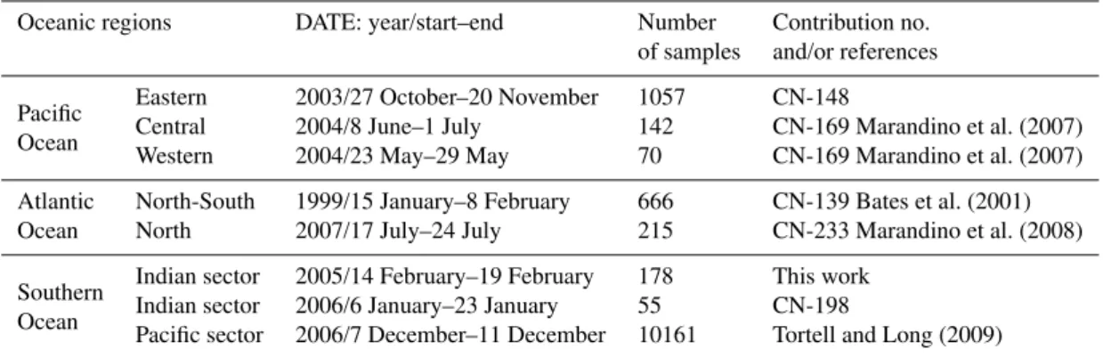
Fig. 1. DMS transects used in this study in conjunction with ocean color and PGD data. Details regarding the data sets can be found in Table 1. The color background is Chl climatology (2002–2007) from the MODIS AQUA sensor.
Table 1.Sea surface DMS datasets used in this study.
Oceanic regions DATE: year/start–end Number Contribution no. of samples and/or references
Pacific Eastern 2003/27 October–20 November 1057 CN-148
Ocean Central 2004/8 June–1 July 142 CN-169 Marandino et al. (2007) Western 2004/23 May–29 May 70 CN-169 Marandino et al. (2007) Atlantic North-South 1999/15 January–8 February 666 CN-139 Bates et al. (2001) Ocean North 2007/17 July–24 July 215 CN-233 Marandino et al. (2008)
Southern Indian sector 2005/14 February–19 February 178 This work Ocean Indian sector 2006/6 January–23 January 55 CN-198
Pacific sector 2006/7 December–11 December 10161 Tortell and Long (2009)
CN: Contribution number to the PMEL global DMS database (http://saga.pmel.noaa.gov/dms/).
measured as described by Kasamatsu et al. (2004). Water samples were collected with a rosette sampler equipped with 20-L Niskin bottles and a conductivity, temperature, depth (CTD) probe (Falmouth Scientific, Inc.). Surface seawater was also collected through the ship’s pumping system from a depth of approximately 5 m. No significant difference in the DMS data collected from these different samplers was found. In the Indian sector of the Southern Ocean, DMS data were obtained during a transit from Kerguelen Island to La R´eunion (Fig. 1) after the KEOPS cruise (Belviso et al., 2008). Water samples were collected underway by means of the Marion Dufresne II’s clean seawater supply line used currently for CO2 fugacity measurements at approximately
5m depth. A comparison was conducted between the clean seawater system (pump samples) and the CTD rosette sam-pler (bottle samples) during the KEOPS cruise. The
analyti-cal protocol is described in Belviso et al. (2008). Figure S2 shows the effects of the clean seawater pumping system on the concentrations of total DMSP (DMSPt) and DMS, re-spectively. No gain or loss of DMSPt in the seawater circuit is observed because DMSPt data points fall close to the 1:1 line (Fig. S2a). On the contrary, DMS concentrations are generally higher in the clean water circuit than in CTD bot-tles (Fig. S2b). It is highly unlikely that the gain in DMS results from a filtration artifact because both the bottle sam-ples and pump samsam-ples were treated similarly. DMS concen-trations from the bottle and pump samples are linearly cor-related. The slope of the relationship (DMSbottle:DMSpump)
the existence of a positive intercept because it would sug-gest that DMS is lost in the pump circuit at very low seawa-ter DMS levels. On the contrary, the relationship shows a general gain of DMS in the pump circuit. In consequence, there are no physical or statistical reasons to reject the equa-tion [DMS]bottle= 0.65×[DMS]pump(r2= 0.89,n=29,P <
0.0001) which results from the forcing of the regression line through zero (Fig. S1b). Hence, a correction factor of 0.65 was applied to this specific set of underway measurements of DMS.
The overall precision of the DMS measurements is ap-proximately ±10%. The instrument deployed at sea by Tortell and Long (2009) displays a higher detection limit (ca. 1 nM) than the other instruments (ca. 0.1 nM). Upper mixed layer DMS measurements are depth compatible with the ocean color measurements made by satellites.
2.2 Satellite observations of ocean color and PGD 2.2.1 Ocean color
Ocean color composites used in this study were computed from SeaWiFS daily L3-binned GAC data between 1997 and 2007 (9 km horizontal resolution, processing version 5.2 n – http://oceancolor.gsfc.nasa.gov/). Chl from SeaWiFS has an uncertainty of ca. 30%. No attempt was made here to compare SeaWiFS Chl data with ship chlorophyll measure-ments because (1) ship-based measuremeasure-ments were not avail-able along each cruise track and (2), when availavail-able, there was no unification of the Chl measurement protocol and the Chl fluorescence sensors were not always calibrated. More-over, diurnal fluorescence values exhibit light-dependent de-pressions resulting from non-photochemical quenching pro-cesses, so fluorescence-based Chl estimates are restricted to nighttime data. This was especially true in the eastern equa-torial Pacific during cruise CN-148 (Behrenfeld and Boss, 2006).
2.2.2 PGD
The PHYSAT method (Alvain et al., 2005) was used to ob-tain composites of PGD along transects presented in Fig. 1. It is based on classical ocean color measurements in the visi-ble spectrum and allows the classification of specific spectral anomalies (for Chl<4 mg m−3and clear sky conditions) de-fined as:
nLw∗(λ)=nLw(λ)/nLwref(λ,Chl)
where nLw(λ) is the spectral water-leaving radiance and nLwref(λ, Chl) is a simple model of nLw(λ) that accounts
only for the Chl concentration. Using this relationship, the first order signal variation (a function of Chl) is removed and the second order variation from the total nLw(λ) spectra vari-ability is isolated and defined by nLw∗(λ). Specific shapes
and amplitudes of nLw∗(λ) have been associated with
spe-cific dominant phytoplankton groups using in situ measure-ments of biomarkers pigmeasure-ments determined by HPLC.
The PHYSAT algorithm was applied to the SeaWiFS daily L3-binned GAC data archive from 1997 to 2007 to identify the following dominant phytoplankton groups in surface waters (Alvain et al., 2005, 2008): Prochlorocco-cus (PRO), SynechococProchlorocco-cus (SYN), nanoeucaryotes (NANO), Phaeocystis-like (PHAEO), coccolithophores (COC), and di-atoms (DIAT). Daily records of phytoplankton groups at a resolution of 1/12◦were used to generate monthly compos-ites of dominant phytoplankton group at 1/4◦by selecting the most frequently detected group for at least half of the valid (including unidentified) pixels. Note that when unidentified pixels prevail or when no phytoplankton group dominates, no PGD is assigned to a grid box.
by the PHYSAT method, are screened to remove the sus-pended calcite signal using a threshold on nLw(λ), so that the PHYSAT results likely underestimate the actual size of coccolithophore blooms (Alvain et al., 2008).
To obtain sufficient data for this study, we have used the best satellite products available at the time of the study and applied no temporal and spatial regridding procedure. Sea-WiFS data have been matched with DMS measurements ac-cording to date (month) and geographical coordinates.
3 Results
Both the climatological and cruise specific data are presented below. Monthly sea surface Chl concentrations and clima-tological (1998–2006) monthly PGD data are used to illus-trate the regional context of the field studies (Sect. 3.1) in three broad areas: Equatorial Pacific and eastern North Pa-cific Ocean, North and South Atlantic Ocean, and the Indian and Pacific sectors of the Southern Ocean. Chl and PGD data extracted from the satellite records along the track of each survey, according to the date (month-year) of the DMS mea-surements, are used for subsequent comparison with DMS field observations (Sect. 3.2).
3.1 Overview of main patterns of chlorophyll and PGD at the regional scale
3.1.1 Equatorial Pacific and eastern North Pacific Ocean
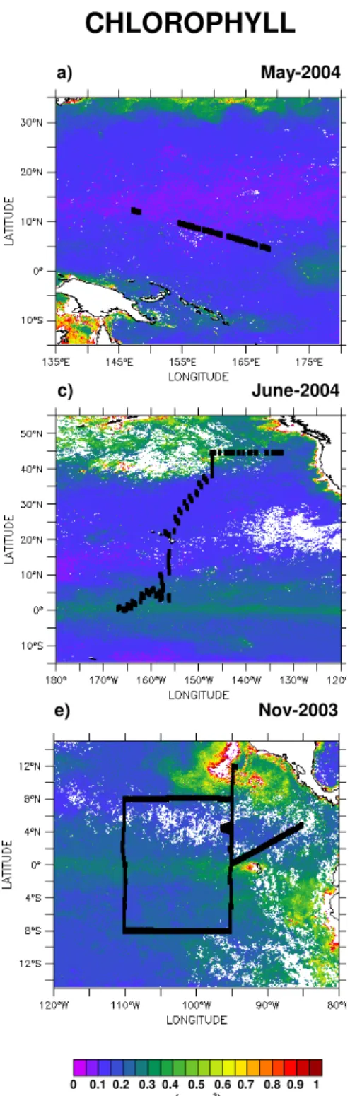
The first track cut across the western warm pool (WWP) of the Equatorial Pacific during the spring season. Ultra-oligotrophic (Chl<0.1 mg m−3) and oligotrophic waters
(Chl∼0.1 mg m−3) occupied the center of the zone (Fig. 2a). Mesotrophic and eutrophic waters (0.15<Chl<1 mg m−3) were found north of 30◦N, around Papua New Guinea and at the equator at 175◦E (Fig. 2a). Climatological PGD in this region also showed latitudinal variations (Fig. 2b). The PHYSAT monthly climatology is investigated here because the monthly maps coinciding with the cruise tracks would have shown too many empty pixels because of cloud cov-erage and high aerosol loading of the atmosphere. NANO dominated north of 30◦N and around Papua New Guinea. The center of the zone was occupied by SYN where most of the DMS measurements were made. In between the two zones, there was a 5◦-wide zone where PRO dominated
(around 25◦N, Fig. 2b) and a much wider zone south of 5◦N
where PRO and SYN alternated over short distances. The cruise ended in a mixed PRO-SYN zone.
In the central North Pacific during early summer 2004, oligotrophic waters were found between 10◦N and 35◦N (North Pacific Gyre (NPG), Fig. 2c). The transition from oligotrophy to mesotrophy was not the same northward (to-wards subtropical waters and the North American coasts) or southward (towards the equatorial divergence zone) in terms
of PGD (Fig. 2d). Northward, there was a band dominated by PRO and NANO. Some areas with concentrated levels of DIAT were also observed there. Southward, there were no marked changes in PHYSAT PGD. Oligotrophic waters of the NPG and the more productive waters near the equator displayed the same mixture of SYN and PRO dominances. SYN dominance prevailed in the zone west of 170◦W be-tween 10◦N and 25◦N.
In November 2003, mesotrophic waters were found off the Central and South American coasts and along the equator (Fig. 2e). The main features in PGD in this region were: (1) NANO dominated off Central America, (2) DIAT dom-inated off Peru, and (3) PRO domdom-inated along the equator (Fig. 2f). SYN dominance prevailed south of 4◦S and west of 100◦W. The DMS survey was carried out mostly in the mixed SYN-PRO zone.
3.1.2 North and South Atlantic Ocean
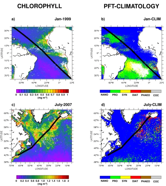
The January 1999 Chl map (Fig. 3a) shows three zones of high productivity (Guinea dome, Benguela upwelling and the equatorial divergence) and two zones of low productiv-ity (north and south subtropical gyres). The ship did not cut across the ultra-oligotrophic waters of the South Atlantic gyre (Chl<0.1 mg m−3). In January, the oligotrophic waters
of the North Atlantic gyre (20◦N) exhibited PRO dominance
(Fig. 3b) while the northern edge of the South Atlantic gyre exhibited PRO and NANO dominances. Elsewhere, NANO dominance prevailed especially in the productive tropical and equatorial waters. In summer, the western North Atlantic is a biologically productive region with Chl concentrations north of 44◦N rising up to 2 mg m−3(Fig. 3c). The PHYSAT cli-matology of the area shows a general prevalence of NANO west of 40◦W and in the Labrador Sea (Fig. 3d). Diatoms were confined to the northeast quarter of the investigated area. Hence, according to the PHYSAT climatology, there were NANO blooms west of 40◦W and DIAT blooms east of 40◦W. Coccolithophores are dominant only over the Ice-landic shelf. The DMS survey covered the NANO and mixed DIAT-NANO zones.
CHLOROPHYLL
PFT-CLIMATOLOGY
a) May-2004 b) May-CLIM
c) June-2004 d) June-CLIM
e) Nov-2003 f) Nov-CLIM
NANO PRO SYN DIAT PHAEO COC 0 0.1 0.2 0.3 0.4 0.5 0.6 0.7 0.8 0.9 1
(mg m-3)
Fig. 2.Regional monthly composites of Chl concentration (left panels, units mg m−3) and monthly climatological composites (1998–2006) of the dominant phytoplankton groups detected by PHYSAT (right panels).(a, b)western Equatorial Pacific,(c, d)central Equatorial Pacific and eastern North Pacific,(e, f)eastern Equatorial Pacific. Dominant phytoplankton groups are: nanoeucaryotes (NANO), Prochloroccocus (PRO), Synechococcus (SYN), diatoms (DIAT), Phaeocystis-like (PHAEO) and coccolithophores (COC).
to the south (Fig. 4d). However, between 20◦E and 70◦E and south of 64◦S, DIAT dominance is replaced by NANO dom-inance (Fig. 4d). PHYSAT domdom-inances alternate between PRO, SYN, NANO and DIAT over short distances in the
a) Jan-1999 b) Jan-CLIM
NANO PRO SYN DIAT PHAEO COC (mg m-3)
c) July-2007 d) July-CLIM
0 0.2 0.4 0.6 0.8 1.0 1.2 1.4 1.6 1.8 2
CHLOROPHYLL
PFT-CLIMATOLOGY
NANO PRO SYN DIAT PHAEO COC 0 0.1 0.2 0.3 0.4 0.5 0.6 0.7 0.8 0.9 1
(mg m-3)
Fig. 3.Same as Fig. 2 but for the Atlantic Ocean.(a, b)North and South Atlantic,(c, d)western North Atlantic.
3.2 DMS:Chl and PHYSAT monthly PGD data extracted along cruise tracks
The spatial and temporal variations of the following param-eters were investigated: sea surface temperature (SST), sea surface salinity (SSS) (when necessary to better characterize the water masses), Chl concentration from SeaWiFS, PGD from PHYSAT, DMS concentration and DMS concentration normalized to satellite Chl concentration (DMS:Chl). Here Chl is used has a field metric for phytoplankton biomass, al-though Chl variability can be strongly influenced by phys-iological shifts in intracellular pigmentation in response to changing growth conditions (light, nutrients, tempera-ture). In the eastern equatorial Pacific Ocean (CN-148, Fig. 1), Behrenfeld and Boss (2006) demonstrated that the
CHLOROPHYLL
PFT-CLIMATOLOGY
a) Feb-2005 b) Feb-CLIM
c) Jan-2006 d) Jan-CLIM
e) Dec-2006 f) Dec-CLIM
NANO PRO SYN DIAT PHAEO COC 0 0.1 0.2 0.3 0.4 0.5 0.6 0.7 0.8 0.9 1
(mg m-3)
Fig. 4.Same as Fig. 2 but for the Indian and Pacific sectors of the Southern Ocean. (a, b, c, d)Indian sector of the Southern Ocean,(e, f) Pacific sector of the Southern Ocean.
3.2.1 Indian and Pacific sectors of the Southern Ocean Indian sector of the Southern Ocean
Approximately 200 seawater samples were analyzed for DMS along the cruise track of RV Marion Dufresne II in late February 2005 between the islands of Kerguelen and Crozet, and across the frontal system north of Crozet Island
33.5 34 34.5 35 35.5 36 5 10 15 20 25 -47 -45 -43 -41 -39 -37 SSS SST (°C) 33.5 33.6 33.7 33.8 33.9 4 5 6 7 8 9
52 54 56 58 60 62 64 66 68 70
SST (°C) SSS 0 0.1 0.2 0.3 0.4 0.5 0.6 0.7 0 1 2 3 4 5 6 7 -47 -45 -43 -41 -39 -37
Chl (mg m
-3) DMS (nM)
0 0.2 0.4 0.6 0.8 1 1.2 0 1 2 3 4
52 54 56 58 60 62 64 66 68 70
DMS (nM)
Chl (mg m
-3) 0 5 10 15 20 25 30 NANO PRO SYN DIAT -47 -45 -43 -41 -39 -37 Latitude
DMS:Chl (mmol g
-1) PHYSAT
PGD 0 5 10 15 20 25 NANO PRO SYN DIAT PHAEO
52 54 56 58 60 62 64 66 68 70
Longitude (°E)
PHYSAT
PGD
DMS
:Chl (mmol g
-1) CROZET CROZET KERGUELEN AF STF SAF warm core eddy
a
c
e
b
d
f
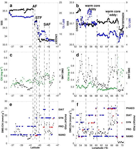
warm core eddyFig. 5.Spatial variations of(a, b)sea surface temperature (SST:◦C, in blue) and salinity (SSS, in black),(c, d)ocean color (Chl: mg m−3, in green) and sea surface dimethylsulfide concentration (DMS: nM, in black),(e, f)DMS-to-Chl ratio (DMS:Chl, mmol g−1, in black) and monthly (red dots) and monthly climatological (blue dots) composites of phytoplankton group dominance along two DMS transects carried out in February 2005 in the Indian Sector of the Southern Ocean (right panels: longitudinal transect between Kerguelen and Crozet, left panels: latitudinal transect between Crozet and La R´eunion). AF: Agulhas front, STF: subtropical front, SAF: subantarctic front.
(<200 m) over the Kerguelen Plateau, north of the polar front during a phytoplankton bloom (Fig. 5d, see also Park et al., 2008). DMS:Chl are as low as 0.5 mmol g−1there (Fig. 5f).
Unfortunately, few PHYSAT data were available in this area to evaluate the PGD in the bloom area (Fig. 5f). However, climatological data suggest NANO or SYN dominance but not DIAT or PHAEO. In the warm core eddy over the slope (200 m−2000 m depth) between 65◦E and 68◦E (Fig. 5b), Chl levels were 2-6-fold lower than over the plateau. The DMS trend is the exact opposite (Fig. 5d). DMS:Chl peaks over the slope with values up to 22 mmol g−1, increasing by a factor of 40 over one degree longitude. The dominant
phytoplankton group was PHAEO both climatologically and during February 2005 data (Fig. 5f). The ship cut across a second warm core eddy between 56◦E and 60◦E (Fig. 5b).
-70 -65 -60 -55 -50 -45 -40 -2 0 2 4 6 8 10 12
Jan/5 Jan/9 Jan/13 Jan/17 Jan/21 Jan/25
Latitude SST (°C) 176 178 180 -178 -176 -174 -172 -2 0 2 4 6 8 10 -66 -64 -62 -60 -58 -56 -54 -52 SST (°C) Longitude 0 0.1 0.2 0.3 0.4 0.5 0.6 0 2 4 6 8 10
Jan/5 Jan/9 Jan/13 Jan/17 Jan/21 Jan/25
Chl (mg m
-3) DMS (nM)
0 0.2 0.4 0.6 0.8 0 1 2 3 4 5 6 7 8 9 10 11 -66 -64 -62 -60 -58 -56 -54 -52 DMS (nM)
Chl (mg m
-3) 0 10 20 30 40 50 NANO PRO SYN DIAT PHAEO
Jan/5 Jan/9 Jan/13 Jan/17 Jan/21 Jan/25
DMS
:Chl (mmol g
-1) PHYSAT PGD Date 0 10 20 30 40 50 NANO PRO SYN DIAT PHAEO -66 -64 -62 -60 -58 -56 -54 -52 PHYSAT PGD Latitude DMS
:Chl (mmol g
-1)
SAF + PF
a
b
c
d
e
f
DMS max.Indian sector of Southern Ocean Pacific sector of Southern Ocean
Fig. 6. Spatial and temporal distributions of the following parameters in the Indian (left panels) and Pacific (right panels) sectors of the Southern Ocean: (a, d)sea surface temperature (SST:◦C, in blue) and latitude/longitude (in black),(b, e)ocean color (Chl: mg m−3, in green) and sea surface dimethylsulfide concentration (DMS: nM, in black),(c, f)DMS-to-Chl ratio (DMS:Chl, mmol g−1, in black) and monthly (red dots) and monthly climatological (blue dots) composites of phytoplankton group dominance. SO: Southern Ocean, SAF: subantarctic front, PF: polar front.
The highest ratios (up to 18 mmol g−1) were measured in a salinity front (Fig. 5b) and were associated with NANO dom-inance (Fig. 5f).
Unfortunately the transects of DMS, Chl (Fig. 5c) and PHYSAT (Fig. 5e) across the three fronts located north of Crozet (Fig. 5a) are not at the same spatial resolution. Some coherence between the February 2005 data and the PHYSAT monthly climatology was found for NANO but not for PRO. NANO dominance was detected between the Agulhas front and the subtropical front in association with two peaks of DMS and Chl which coincided spatially (Fig. 5e). However,
the DMS:Chl was not homogeneous but instead decreased by a factor of three over half a degree of latitude. The DMS:Chl also was highly variable in the transition zone between the Agulhas front and the warm subtropical water but PGD data were not available.
RT/V Umitaka Maru also explored the Indian Sector of
Table 2.Mean DMS:Chl ratios sorted by oceanic regions and by phytoplankton group dominance.
Sampling location Phytoplankton group dominance DMS:Chl ratio in mmol g−1(mean±1 SD; median;n) Student t-testa Contribution number (CN)
or references
NANO PHAEO PRO SYN DIAT
P
A
C
I
F
I
C
North Pacific>20◦N 23.0±11.6; 17.0; 7 – 23.4±7.1; 24.0; 7 12.2±5.4; 11.9; 9 –
CN-169 NS,P= 0.933 NS,P= 0.052
Equatorial Pacific 13.7±2.7; 13.7; 25 – 17.8±9.8; 15.7; 85 14.6±5.0; 13.8; 404 – 8◦S–2◦S, 0◦–16◦N S,P <0.0001 NS,P= 0.148
CN-148, CN-169
Equatorial Pacific 7.0±0.6; 7.1; 10 – 6.2±0.6; 6.3; 44 8.4±2.4; 8.1; 47 –
2◦S–0◦(ED) S,P= 0.003 S,P= 0.0007
CN-148
A
T
L
A
N
T
I
C
North Atlantic 4.6±2.2; 3.9; 88 – 3.2±1.0; 3.0; 15 7.1±2.4; 6.8; 13 4.8±1.5; 4.5; 23
CN-233 S,P= 0.0001 S,P= 0.0028 NS,P= 0.495
Equatorial Atlantic 4.4±1.4; 4.4; 19 – – – –
2◦S–0◦(ED) CN-139
South Atlantic 3.6±3.1; 2.8; 20 – –; 1.8; 2 – –
Benguela Upwelling (BU) CN-139
North & South Atlantic 12.2±11.6; 10.1; 249 – 16.9±8.7; 13.5; 141 13.8±7.8; 12.2; 31 –
except ED & BU S,P <0.0001 NS,P= 0.31
CN-139
A
U
S
T
R
A
L Indian Sector of 12.7±6.3; 12.4; 21 15.1±11.2; 12.2; 13 7.7±1.2; 7.5; 6 6.4±3.8; 6.3; 10 8.2±7.4; 5.5; 8
Southern Ocean NS,P= 0.505 S,P= 0.0016 S,P= 0.0022 NS,P= 0.147
CN-128; this work
Pacific Sector of 9.1±6.9; 8.5; 302 – 23.1±5.3; 23.2; 155 7.6±2.9; 7.7; 851 11.3±4.8; 10.3; 897
Southern Ocean (DEC) S,P <0.0001 S,P= 0.0002 S,P <0.0001
Tortell and Long (2009)
aStudent t-test for unpaired data with unequal variance (NANO vs. other phytoplankton groups). S: significant, NS: non significant,P: t-test probability, DEC: December
spot” (50 mmol g−1) coincided with the sole PHAEO domi-nance of the area (Fig. 6c). In late January, the ship cut across a diatom bloom which was associated with considerably lower ratios (i.e. about a 10-fold decrease was observed be-tween the PHAEO and DIAT areas). The mean DMS:Chl as-sociated with DIAT was highly variable 8.2±7.4 mmol g−1
(n=8).
When the DMS:Chl data sets collected in summer in the Indian sector of the Southern Ocean are pooled together with NANO dominance used as the reference, it is clear that mean DMS:Chl are significantly lower (i.e. about half lower) in SYN or PRO than in NANO dominated areas (Ta-ble 2). Mean DMS:Chl associated with NANO + PHAEO and PRO + SYN + DIAT were 13.6±8.4 mmol g−1(n
=34)
and 7.3±4.8 mmol g−1(n
=24, Table 3), respectively, a sta-tistically significant difference (P=0.0006).
Pacific sector of the Southern Ocean
In December 2006, Tortell and Long (2009) surveyed the lat-itudinal distribution of DMS in the Southern Ocean roughly along the dateline from the Ross Sea up to 53◦S (Fig. 6,
right panels). In the present study, the investigation area is restricted to surface waters free of ice (53◦S and 64◦S). SST decreased steadily with increasing latitude except in the area of the subantarctic and polar fronts (SAF and PF, respectively) which were crossed between 56◦S and 60◦S
Table 3.Mean DMS:Chl ratios sorted by oceanic regions and by phytoplankton group dominance to trace the dominance of high and low DMSP producers.
Sampling location
Contribution number (CN) or references
DMS:Chl ratio in mmol g−1(mean±1 SD; median;n) Student t-testa
High DMSP producers NANO + PHAEO
Low DMSP producers PRO + SYN + DIAT
P
A
C
I
F
I
C
North Pacific>20◦N CN-169
23.0±11.6; 17.0; 7 17.1±8.3; 16.9; 16 NS,P= 0.257 Equatorial Pacific
8◦S–2◦S, 0◦–16◦N CN-148, CN-169
13.7±2.7; 13.7; 25 15.2±6.3; 14.0; 489 S,P= 0.023
Equatorial Pacific 2◦S–0◦(ED) CN-148
7.0±0.6; 7.1; 10 7.4±2.1; 6.6; 91 NS,P= 0.201
A
T
L
A
N
T
I
C
North Atlantic CN-233
4.6±2.2; 3.9; 88 4.9±2.2; 4.4; 51 NS,P= 0.439 Equatorial Atlantic
2◦S–0◦ (ED) CN-139
4.4±1.4; 4.4; 19 – –
South Atlantic
Benguela Upwelling (BU) CN-139
3.6±3.1; 2.8; 20 –; 1.8; 2 S,P= 0.017
North & South Atlantic except ED & BU CN-139
12.2±11.6; 10.1; 249 16.4±8.6; 13.2; 172 S,P <0.0001
A
U
S
T
R
A
L Indian Sector of
Southern Ocean CN-128; this work
13.6±8.4; 12.3; 34 7.3±4.8; 7.3; 24 S,P= 0.0006
Pacific Sector of Southern Ocean (DEC) Tortell and Long (2009)
9.1±6.9; 8.5; 302 10.6±5.8; 9.3; 1903 S,P= 0.0005
aStudent t-test for unpaired data with unequal variance, S: significant, NS: non significant,P: t-test probability, DEC: December
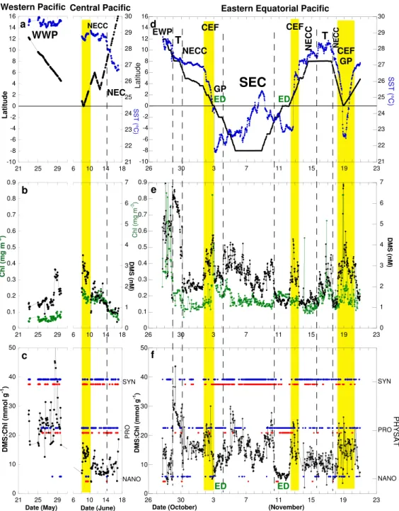
3.2.2 Equatorial Pacific and eastern North Pacific Ocean
In the Pacific western warm pool (WWP), SST was over 29◦C (Fig. 7a) and surface waters displayed low phytoplank-ton biomass (Chl<0.1 mg m−3, Fig. 7b). The DMS:Chl ranged between 13 and 55 mmol g−1 and was on average 25±7.5 mmol g−1 (Fig. 7c, n=65). The PGD alternated between SYN and PRO (Fig. 7c). Climatological (May) and monthly (May 2004) PHYSAT data extracted from maps are in agreement.
In the central Pacific, there was an equatorward positive gradient of SST, Chl and DMS concentrations (Fig. 7a and b). PGD in this region and in the previous one were similar except near the equator where some NANO were detected (Fig. 7c). Although the DMS:Chl ratio was about twice as high a few degrees north of the equatorial divergence zone
(ED) than in the area of the north equatorial counter current (NECC) and the north equatorial current (NEC) (4–15◦N), overall the ratio was 2–3 fold lower in the central than in the western Pacific.
-10 -8 -6 -4 -2 0 2 4 6 8 10 12 14 16 21 22 23 24 25 26 27 28 29 30
21 25 29 6 10 14 18
Latitude SST (°C) 21 22 23 24 25 26 27 28 29 30 -10 -8 -6 -4 -2 0 2 4 6 8 10 12 14 16
26 30 3 7 11 15 19 23
SST (°C) Latitude 0 0.1 0.2 0.3 0.4 0.5 0.6 0.7 0.8 0.9 0 1 2 3 4 5 6 7
21 25 29 6 10 14 18
Chl (mg m
-3 ) DMS (nM) 0 1 2 3 4 5 6 7 0 0.1 0.2 0.3 0.4 0.5 0.6 0.7 0.8 0.9
26 30 3 7 11 15 19 23
DMS (nM)
Chl (mg m
-3) 0 10 20 30 40 50
21 25 29 6 10 14 18 NANO
PRO
SYN
DMS:Chl (mmol g
-1)
Date (May) Date (June)
NANO PRO SYN
26 30 3 7 11 15 19 23
0 10 20 30 40 50 PHYSAT
Date (October) (November)
DMS:Chl (mmol g
-1) EWP NECC NECC
SEC
ED ED a d b e c fWestern Pacific Eastern Equatorial Pacific
WWP GP ED ED CEF CEF GP CEF NECC NEC Central Pacific NECC T T
Fig. 7. Temporal variations of the following parameters in the western and central (left panels cruise CN-169) and eastern (right panels, cruise CN-148) Equatorial Pacific:(a, d)sea surface temperature (SST:◦C, in blue) and latitude (in black),(b, e)ocean color (Chl: mg m−3, in green) and sea surface dimethylsulfide concentration (DMS: nM, in black),(c, f)DMS-to-Chl ratio (DMS:Chl, mmol g−1, in black) and monthly (red dots) and monthly climatological (blue dots) composites of phytoplankton group dominance. The yellow vertical bands correspond to the convergent equatorial front (CEF) where DMS accumulates. WWP: western warm pool, NEC: north equatorial current, EWP: eastern warm pool, NECC: north equatorial counter current, T: transition zone between EWP and NECC, GP: Galapagos plume, ED: equatorial divergence, SEC: south equatorial current.
front (CEF), which separates the warm and light waters of the NECC from the cooler and denser waters of the ED, is an area where DMS accumulates. The CEF was crossed 3 times during the cruise and DMS concentrations were systemat-ically higher there than in the surrounding areas (Fig. 7e).
here, the DMS:Chl ratio (Fig. 7f) was very low. The PGD in the ED varied with longitude. At 95◦W, in the vicinity of
the Galapagos Island (GP, date: 3 and 4 November), SYN dominated whereas far to the west (110◦W) PRO dominated (date: 11 and 12 November). Based on the climatology of PGD, PRO is more typical in the ED than SYN. SYN clearly dominated in the SEC both in November 2003 and in the cli-matology. The occurrence of NANO dominance is rare in the eastern Pacific in November 2003. Whatever the phyto-plankton dominance is in the equatorial Pacific Ocean, mean DMS:Chl were markedly lower in ED than outside of this area (Tables 2 and 3). Mean DMS:Chl were not significantly higher in the presence of high DMSP producers (Table 3).
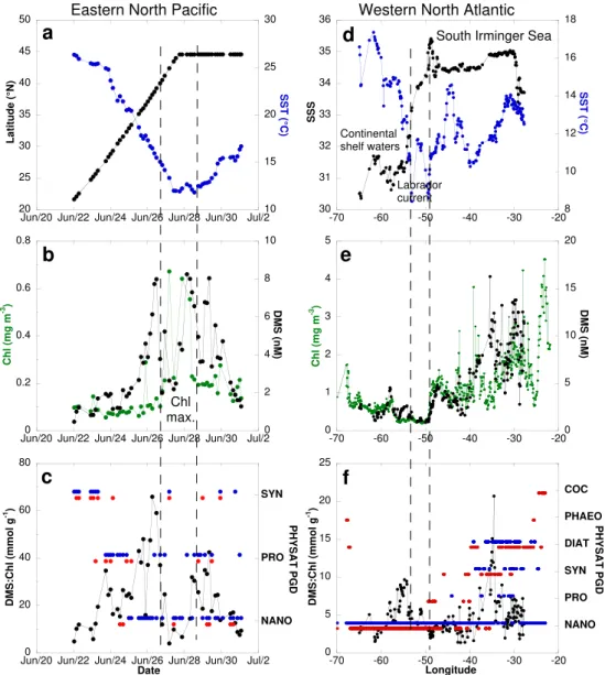
In the eastern North Pacific, the DMS:Chl increased from 5–12 mmol g−1 at 20–25◦N to 58–67 mmol g−1 at about
40◦N, but not steadily (Fig. 8c). The ratio followed the
steady latitudinal decrease of SST (Fig. 8a) and was con-trolled by the DMS concentration (Fig. 8b). An increase in the DMS:Chl, also paralleling the SST but of smaller am-plitude, was observed off the north American coast towards the center of the north Pacific at 45◦N. Between 40◦N and 45◦N, the ratio dropped to low values when the vessel cut across a phytoplankton bloom. Unfortunately, no satellite data were available to produce PHYSAT dominances in this bloom area. Away from this bloom the PGD alternates be-tween NANO, PRO and SYN. We find no significant differ-ence in mean DMS:Chl between NANO and the other dom-inant group, or between high and low DMSP producers (Ta-bles 2 and 3).
3.2.3 North and South Atlantic Ocean
The July 2007 cruise (CN-233) cut across cold (Fig. 8d) and unproductive (Fig. 8e) waters between 49◦W and 53◦W in the Labrador current. This is a transition area separating continental shelf waters (low salinities in the range 30.5– 31.5) from the Atlantic subarctic waters (higher salinities in the range 34–35, Fig. 8c). The lowest DMS levels encoun-tered on this cruise (0.9–1.0 nM) were observed there. A major change in PGD took place at about 45◦W (Fig. 8f). The southwestern sector was dominated by NANO and the DMS:Chl was in the range 2–10 mmol g−1. The northeast-ern sector displayed a larger range (2–20 mmol g−1) and less homogeneous PGD. The six PHYSAT categories were rep-resented in this sector. However, the COC and PHAEO signals were recorded outside the area surveyed for DMS (Fig. 8f). The highest mean DMS:Chl were associated with SYN dominance (Table 2). However, when mean DMS:Chl were sorted between low and high DMSP producers, no sig-nificant difference was observed (Table 3).
The January 1999 cruise (CN-139) cut across a series of currents from 38◦N to 30◦S (Gulf Stream (GS), NECC, SEC and the Benguela current, Fig. 9a). It also crossed the Sargasso Sea, central waters of the north Atlantic subtrop-ical gyre (SG), a westward extension of the Guinea Dome
(GD-ext), the equatorial divergence (ED) and the northern edge of the south Atlantic subtropical gyre before entering the more biologically productive areas off the African coast. The SG waters were poorer in Chl but about twice as rich in DMS than the Gulf Stream and the Sargasso Sea (Fig. 9b) yielding DMS:Chl up to 35 mmol g−1(Fig. 9c). PGD in the SG was mainly PRO. In the northern and southern edges of the north Atlantic SG, PHYSAT dominances alternated be-tween PRO and NANO. The January climatology of PGD depicts a slightly different picture in which PRO is not de-tected north of 25◦N while PRO occurred up to 30◦N in Jan-uary 1999. NANO was the dominant phytoplankton group in the equatorial region from 10◦N to 10◦S. This signa-ture was associated with low DMS:Chl while ED was char-acterized by the lowest values (3 mmol g−1). The northern
edge of the south Atlantic subtropical gyre was dominated by PRO with DMS:Chl ranging between 30 and 50 mmol g−1
(Fig. 9c). However, to the east the influence of the Benguela current (BC) was visible. DMS and Chl highs and lows al-ternated over short distances. While DMS concentrations were over 2 nM everywhere, a clear positive gradient of Chl was observed towards the African coasts. The DMS:Chl ra-tio follows a similar trend since it is mainly controlled by Chl. The lowest ratios were observed in the core of the coastal upwelling (off Namibia) were SST dropped below 16◦C (Fig. 9a). The PGD was NANO in the upwelling area. Offshore it alternated between NANO and PRO. SYN dominance was an extremely rare event in January along the track of the research vessel. We find no significant differ-ence in mean DMS:Chl between NANO and SYN in the At-lantic away from ED and BC (Table 2). On the contrary, the difference between NANO and PRO was highly significant (P <0.0001). The difference between high and low DMSP producers was also highly significant, but in this case the highest mean DMS:Chl was associated with the low DMSP producers (Table 3).
4 Discussion
20 25 30 35 40 45 50
10 15 20 25 30
Jun/20 Jun/22 Jun/24 Jun/26 Jun/28 Jun/30 Jul/2
Latitude (°N)
SST
(°C)
30 31 32 33 34 35 36
8 10 12 14 16 18
-70 -60 -50 -40 -30 -20
SSS
SST
(°C)
0 0.2 0.4 0.6 0.8
0 2 4 6 8 10
Jun/20 Jun/22 Jun/24 Jun/26 Jun/28 Jun/30 Jul/2
Chl (mg m
-3) DMS (nM)
0 1 2 3 4 5
0 5 10 15 20
-70 -60 -50 -40 -30 -20
Chl (mg m
-3) DMS (nM)
0 20 40 60 80
NANO PRO SYN
Jun/20 Jun/22 Jun/24 Jun/26 Jun/28 Jun/30 Jul/2
DMS:Chl (mmol g
-1)
PHYSAT
PGD
Date
0 5 10 15 20 25
NANO PRO SYN DIAT PHAEO COC
-70 -60 -50 -40 -30 -20
DMS
:Chl (mmol g
-1)
PHYSAT
PGD
Longitude
a
b
c
d
e
f
Chl max.
Eastern North Pacific Western North Atlantic
Continental shelf waters
South Irminger Sea
Labrador current
Fig. 8. Spatial or temporal distributions of the following parameters in the eastern North Pacific (left panels, cruise CN-169) and western North Atlantic (right panels, cruise CN-233):(a, d)sea surface temperature (SST:◦C, in blue), latitude (in black), and sea surface salinity (PSU, in black)(b, e)ocean color (Chl: mg m−3, in green) and sea surface dimethylsulfide concentration (DMS: nM, in black),(c, f) DMS-to-Chl ratio (DMS:Chl, mmol g−1, in black) and monthly (red dots) and monthly climatological (blue dots) composites of phytoplankton group dominance.
4.1 PGD control on DMS:Chl variability in the Atlantic Ocean
First, in the subtropical and tropical Atlantic Ocean away from the equatorial divergence and the Benguela current, data showed higher (ca. 40%) mean DMS:Chl with PRO than with NANO dominance (Table 2). Moreover, DMS:Chl up to 35 mmol g−1were observed in the North Atlantic subtrop-ical gyre in winter (Fig. 9c). In the Sargasso Sea, where the dominant PHYSAT signature was NANO, the ratio ranged between 2 and 8 mmol g−1 (Fig. 9c). Similar values were reported by Le Clainche et al. (2010) at the Bermuda At-lantic Time Series (BATS, 32◦N–64◦W) site during
-40 -30 -20 -10 0 10 20 30 40
16 18 20 22 24 26 28
15 19 23 27 31 4 8
Latitude
SST (°C)
0 0.2 0.4 0.6 0.8
0 1 2 3 4 5 6 7
15 19 23 27 31 4 8
Chl (mg m
-3 ) DMS (nM)
0 10 20 30 40 50 60
NANO PRO SYN
15 19 23 27 31 4 8
DMS:Chl (mmol g
-1 )
PHYSAT
Date (January) (February)
ED
NECC GD-ext
ED
SG
Sargasso Sea GS
SEC
Benguela currentED
a
b
c
SG
Fig. 9.Temporal variations of the following parameters in the north and south Atlantic Ocean (cruise CN-139):(a)sea surface temperature (SST:◦C, in blue) and latitude (in black),(b)ocean color (Chl: mg m−3, in green) and sea surface dimethylsulfide concentration (DMS: nM, in black),(c)DMS-to-Chl ratio (DMS:Chl, mmol g−1, in black) and monthly (red dots) and monthly climatological (blue dots) composites of phytoplankton group dominance. Chl levels over 0.8 mg m−3were up to 2.7 mg m−3and 9.1 mg m−3off the North American and South African coasts, respectively. DMS levels over 7 nM were up to 10.1 nM and 11 nM on 3 and 7 February, respectively. GS: Gulf stream, SG: subtropical gyre, GD-ext: Guinea dome extension, NECC: north equatorial counter current, ED: equatorial divergence, SEC: south equatorial current.
the PRO dominated areas (Fig. 9c). Thus, it is likely that the seasonal expansion towards the north of the PRO signa-ture, as observed by Alvain et al. (2008) in the North Atlantic basin, traces that of oligotrophic systems and the well known associated relative accumulation of DMS that characterizes them (summer DMS paradox, Sim´o and Pedr´os-Ali´o, 1999). The expansion of the PRO signature reaches the BATS sta-tion in summer where the relative accumulasta-tion of DMS over DMSP and Chl peaks (Dacey et al., 1998).
it is impossible to assess the relative contribution of coccol-ithophores to phytoplankton biomass during CN-233. Nev-ertheless, the distribution of calcifying and silicifying phy-toplankton in relation to environmental and biogeochemi-cal parameters during the late stages of the 2005 north At-lantic spring bloom was investigated by Leblanc et al. (2009). The spatial distributions of fucoxanthin, biogenic silica, 19’-hexanoyloxyfucoxanthin, particulate inorganic carbon (cal-cite) and peridinin concentrations, showed that diatoms dom-inated the phytoplankton community over prymnesiophytes, coccolithophores and autotrophic dinoflagellates in the Ice-landic basin and shelf in early July. Hence, satellite prod-ucts and ship-based observations in the western North At-lantic in summer suggest that coccolithophores account for a non-dominant fraction of phytoplankton. Thus, the mean DMS:Chl in DIAT dominated areas (4.8±1.5 mmol g−1,
Ta-ble 2) could result from the production of DMS by coc-colithophores (DMS vs. calcite relationship of Marandino et al., 2008 which supports earlier findings of Matrai and Keller, 1993) with diatoms responsible for the high chloro-phyll levels. In the study of Vogt et al. (2008) carried out in a Norwegian Fjord, the phytoplankton bloom was also dominated by diatoms and prymnesiophytes, including lithed Emiliania huxleyi cells. At the highest DMS con-centrations, the DMS:Chl were in the range 1–2 mmol g−1. During the KEOPS study carried out over the Kerguelen Plateau, the iron-fertilized diatom bloom was high in Chl (ca. 1.3 mg m−3) but low in DMS (ca. 0.6 nM, Belviso et al., 2008). There, DMS:Chl were lower than 1 mmol g−1 because the DMS precursor (DMSP) was associated with a non-dominant fraction of phytoplankton made of small sized eucaryotes and single cells ofPhaeocystis antarctica. In ice-free waters of the Barents Sea (station IV) where diatoms ac-counted for about 80% of phytoplanktonic carbon biomass, the sea surface DMS:Chl was ca. 3.5 mmol g−1(Matrai and Vernet, 1997). Consequently, a mean DMS:Chl equal to 4.9±2.2 mmol g−1measured during CN-233 (Table 3) is a relatively high number for an area dominated by low DMSP producers. Surface ocean DMS observations in COC dom-inated areas are definitely required to improve assessment of the ability of PHYSAT to predict temporal and spatial changes in DMS associated with COC blooms.
Third, approaching the coastal upwelling of southern Benguela, the gradient in DMS:Chl was negative in the on-shore direction and PGD was NANO in a large majority of cases (Fig. 9c and Table 2). Although no DIAT dom-inance was found along cruise track, it is likely that di-atoms accounted for a significant fraction of phytoplankton biomass, at least at inshore localities (Barlow et al., 2005), so that DIAT dominance could also be associated with low DMS:Chl. A similar decrease in DMS:Chl with diatom dom-ination of the microplankton biomass was found off Mauri-tania at about 18◦N (Franklin et al., 2009). Hence, PGD would not be the most important control on the variabil-ity of the DMS:Chl in the coastal upwelling of southern
Benguela. In the upwelling off the Moroccan coast, a tran-sect through different plumes of upwelled waters and six longshore traverses of the same plume were carried out in September 1999 (Belviso et al., 2003). It was concluded that DMSP was homogeneously distributed amongst plank-tonic communities, because the sea surface concentration of total DMSP (tDMSP) was highly correlated with the total volume of suspended particles measured by an optical HIAC counter. The uniformity of the ratio between tDMSP and the volume of suspended particles in surface waters contrasted with the high variability of the DMS:Chl and DMS:tDMSP ratios. The ratios decreased in the onshore direction both in the plume and in an adjacent water mass. Marine CO2levels
suggested that the age of the upwelled waters was the main control on the variability of the ratios there, but not the phy-toplankton community composition (Belviso et al., 2003).
Fourth, DMS:Chl were also especially low in the Equato-rial Atlantic divergence zone were NANO dominance was observed (Fig. 9c and Table 2). The meridional distribu-tions of DMS:Chl in a 10◦-wide band around the equator, at 15–35◦W in the Atlantic, 95◦W and 110◦W in the Pa-cific are shown in more detail in Fig. 10a and b, respectively. Abrupt decreases in DMS:Chl were observed when enter-ing the equatorial divergence zone (3 mmol g−1 in the At-lantic and 5 mmol g−1in the Pacific) from the north (NECC) or from the south (SEC). The latitudinal trends in DMS:Chl were similar in the two basins, yet PGD was different (SYN and PRO in the Pacific, NANO in the Atlantic).
We therefore conclude that DMS, Chl and PGD data gath-ered in the Atlantic Ocean provide no evidence that phyto-plankton dominance determined from satellite measurements controls DMS:Chl variability in this basin.
4.2 PGD control on DMS:Chl variability in the Pacific Ocean
DMS:Chl variability in the Pacific Ocean is even less affected by PGD than in the Atlantic Ocean (Table 3). There is only about a 10% difference in mean DMS:Chl between high and low DMSP producers in the equatorial Pacific away of the equatorial divergence zone. The decrease in DMS:Chl in the equatorial divergence is striking but it does not result from changes in phytoplankton group dominance (Table 3).
0 5 10 15 20 25 30 35
NANO PRO SYN
-10 -8 -6 -4 -2 0 2 4 6 8 10
DMS:Chl (mmol g
-1)
PHYSAT
Latitude 95°W
110°W
SEC ED CEF NECC
110°W
95°W
0 5 10 15 20
NANO PRO SYN
-10 -8 -6 -4 -2 0 2 4 6 8 10
DMS:Chl (mmol g
-1 )
PHYSAT
Latitude
SEC ED NECC
Equatorial Pacific
Equatorial Atlantic
a
b
Fig. 10. (a)Latitudinal variations in DMS:Chl at 110◦W and at 95◦W (empty and full circles, respectively) and phytoplankton group dominance (blue circles and red crosses, respectively) in the Equatorial Pacific.(b)Same as (a) but in the Equatorial Atlantic between 15◦ and 35◦W. NECC: north equatorial counter current, ED: equatorial divergence, CEF: convergent equatorial front, SEC: south equatorial current.
chlorophyll was functioning as a reliable measure of phyto-plankton biomass in the eastern equatorial Pacific in Novem-ber 2003 (Behrenfeld and Boss, 2006). Indeed, the partic-ulate beam attenuation coefficient (cp), a measure of
sus-pended material mostly of phytoplanktonic origin, was ex-tremely well correlated with fluorescence-based chlorophyll estimates (Fig. S3a,r2= 0.93,n=8,880) over the 6600 km transect. As Fig. S3c shows,cpwas less correlated with DMS
than with Chl (r2= 0.19,n=424). However, when ED data is removed, the coefficient of determination of DMS vs.cp
markedly increases (r2= 0.40,n=375, Fig. S3d). Therefore, ED data have a stronger impact on the DMS vs.cp
relation-ship than on that between Chl andcp. This provides
inde-pendent support for the existence of a reduction in the ED of the DMS:Chl calculated from ocean color data. The highly significant linear relationship observed between total partic-ulate organic carbon andcp (see Fig. 4b in Behrenfeld and
ED (Table 3). This points toward a driving process that is not common to Chl and DMS. The eastern equatorial Pacific zone is characterized by a major plume of nutrient rich wa-ter located mostly south of the Equator. There, mean sur-face nitrate concentrations are over 5 µM in the longitudinal band 95◦W–110◦W (Fiedler and Talley, 2006). Since ni-trate photolysis is related to DMS photochemistry (Bouillon and Miller, 2004), it is possible that an enhancement in ni-trate concentration increases the photochemical removal ef-ficiency of DMS resulting in lower DMS concentrations in the surface ocean. Thus, the DMS dynamics in the eastern equatorial Pacific would be impacted by physical and chemi-cal forcings more directly than by physiologichemi-cal and ecologi-cal processes. Because the latitudinal variations in DMS:Chl are roughly the same in the equatorial Atlantic and Pacific, it is suggested that the decoupling between DMS and phy-toplankton biomass observed in the equatorial Pacific also operates in the equatorial Atlantic though we lack the sup-porting material (e.g.cp measurements, indices of changes
in algal physiology) in this latter case.
The Pacific convergent equatorial front (CEF) is a tran-sition zone between the eastward-flowing NECC and the westward-flowing SEC. It is located north of the equator and, as our results show, is a place where gradients in DMS:Chl are especially steep. Moreover, in the central Pa-cific (at 140◦W) where SST gradients were considerably weaker than at 95◦W and 110◦W (Fig. 7a), the ratio still rose markedly between 0◦ and 2◦N (Fig. 7c). It is known that the CEF accumulates buoyant organic material that can be seen from space and attracts foraging seabirds and other trophic level species (Pennington et al., 2006 and references therein). Clearly, DMS accumulates there too. This is con-sistent with the idea that DMS serves as a foraging cue for seabirds (Nevitt et al., 1995). When zooplankton prey upon phytoplankton rich in DMSP and in DMSP-lyases, part of the particulate material is released to solution and converted to DMS. Nanoeucaryotes are richer in DMSP and lyases than cyanophytes and prochlorophytes. This is true on a per cell basis, or when DMSP is normalized to cell carbon or chloro-phyll (Stefels et al., 2007). Because PHYSAT dominance in the equatorial Atlantic is NANO and because chlorophyll levels are slightly higher in the Atlantic than in the Pacific, higher phytoplankton production of DMS is expected in the Atlantic than in the Pacific. Therefore, the Atlantic should display higher DMS levels than the Pacific. Definitely, this is not the case in equatorial waters as the comparison of Fig. 7e and Fig. 9b shows. Consequently, phytoplankton dominance does not control the concentration of DMS in equatorial wa-ters neither in absolute nor in relative (when normalized to Chl concentration). It appears that the upper ocean dynamics near the equator is important in two aspects: upwelling areas are not favorable for DMS accumulation whereas convergent fronts are important.
Since the equatorial Pacific Ocean is subject to large inter-annual variations in upper ocean dynamics during El Ni˜no-Southern Oscillation (ENSO) cycles, it is expected that the spatio-temporal DMS distribution will change accordingly. Indeed, there appears to be large changes in DMS in the vicinity of the equatorial divergence during El Ni˜no and La Ni˜na events as shown from historical data gathered in Fig. S4. During non El-Ni˜no events (La Ni˜na or transition phase), data collected between the equator and 5◦N, at the position of the convergent front, show an accumulation of DMS of varying intensity (4–11 nM) in the central (140◦W, Fig. S4a) and eastern (110◦W, Fig. S4b) Equatorial Pacific. This local accumulation apparently disappears during El-Ni˜no events (1.2–2.3 nM) suggesting a relationship between ENSO cycles and the DMS distribution. However, the DMS loss at the location of the convergent equatorial front dur-ing El-Ni˜no events can be partly compensated by an increase in DMS in the area of the equatorial divergence at 110◦W
(Fig. S4b, April 1983). No such compensation is observed at 140◦W in March 1992 (Fig. S4a). Hence, the changes in physical features associated with ENSO events appear to have a stronger effect on the concentration of DMS at the lo-cal slo-cale than over large distances across the Equatorial Pa-cific (Bates and Quinn, 1997). These results provide after Wong et al. (2006) a new example of how climate fluctua-tions, through altering the physical properties of the upper ocean, may influence the DMS concentrations in the open ocean. SeaWiFS and PHYSAT surveys show a marked drop in phytoplankton biomass and a shift from SYN to NANO in the equatorial Pacific during El Ni˜no events (Masotti et al., 2010). Since DMS concentrations and the phytoplankton biomass drop simultaneously, the ratio of both is expected to remain roughly constant. Therefore, a shift from SYN to NANO during El Ni˜no events would not be expected to effect the DMS:Chl ratio. This is consistent with our observations which show no significant difference (P=0.148) in mean sea surface DMS:Chl exhibiting SYN (14.6±5.0 mmol g−1) and NANO dominances (13.7±2.7 mmol g−1, Table 2). 4.3 PGD control on DMS:Chl variability in the
Austral Ocean
a much higher contrast in DMS:Chl when phytoplankton is sorted in categories of low and high DMSP producers, espe-cially in the high latitudes in summer when NANO and/or COC bloom (Fig. S1a and b).
5 Conclusion and perspectives
The PHYSAT tool allows the characterization at the global scale of dominant phytoplankton groups. It was applied for the first time to the marine sulfur cycle in an effort to assess whether variability in the DMS:Chl ratio is consistent with the distribution of dominant phytoplankton groups as deter-mined from space. Based on this survey, the Indian sector of the Southern Ocean is the only region where the spatial variations in the DMS:Chl ratio appear to be consistent with the generally accepted classification between high and low DMSP-producing phytoplankton. There, the ratios in SYN-dominated areas are roughly one half of those in NANO- and PHAEO-dominated areas. Overall, our results indicate that phytoplankton group dominance is not the primary controller of DMS dynamics over most of the oceans. We therefore conclude that ocean color sensor measurements of Chl con-centrations and dominant phytoplankton groups can not be used to predict global fields of DMS.
The spatial resolution of the PHYSAT records will im-prove markedly in the near future. The new PHYSAT prod-ucts will display 4 to 9 km horizontal resolution. The tem-poral resolution should be also improved (daily observation matchup) to investigate times when the succession of phy-toplankton groups is happening quickly. This will offer a new opportunity to investigate the effect of phytoplankton dominance on the small-scale distribution of DMS especially in coastal waters. Moreover, future remote sensing stud-ies should focus on characterization of the total ton biomass, the non-dominant component of phytoplank-ton assemblages, the physiological state and the develop-ment stages of phytoplankton, and the environdevelop-mental factors controlling DMS removal processes. For example, particu-late backscattering and calcite products, phytoplankton fluo-rescence, colored dissolved organic material and irradiance below clouds would be useful. Bacteria are important or-ganisms in DMS biogeochemistry but, unfortunately, the as-sessment of bacterial biomass and activity is not yet possible from remote sensing.
Supplementary material related to this article is available online at:
http://www.biogeosciences.net/7/3215/2010/ bg-7-3215-2010-supplement.pdf.
Acknowledgements. We gratefully acknowledge scientists, officers and crew aboard R. V. Marion Dufresne for their help during the cruise KEOPS. In particular, we extend our thanks to the project leader, S. Blain, and to the chief scientist, B. Qu´eguiner. The
authors thank NASA/GSFC/DAAC for providing access to daily L3 SeaWiFS binned products. We also thank Patrick Brockmann for assistance in the data management and M. J. Behrenfeld and E. Boss for making beam attenuation coefficient (cp) data
available on line at http://www.science.oregonstate.edu/ocean. productivity/field.data.fl.online.php. We express our special thanks to X. W. Wang who computed for us the spatial distribution of the sea surface C:Chl ratio in the eastern Equatorial Pacific for November 2003. We thank also L. Bopp and M. Vogt for making PISCES and PlankTOM5 modeling data available for us. We thank the two anonymous reviewers for their constructive comments and suggestions to help improving the manuscript. This is LSCE contribution number 4056.
Edited by: T. J. Battin
The publication of this article is financed by CNRS-INSU.
References
Alvain, S., Moulin, C., Dandonneau, Y., and Br´eon, F. M.: Remote sensing of phytoplankton groups in case 1 waters from global SeaWiFS imagery, Deep Sea-Res. Pt. I, 52, 1989–2004, 2005. Alvain, S., Moulin, C., Dandonneau, Y., and Loisel, H.: Seasonal
distribution and succession of dominant phytoplankton groups in the global ocean: A satellite view, Global Biogeochem. Cy., 22, GB3001, doi:10.1029/2007GB003154, 2008.
Barlow, R., Sessions, H., Balarin, M., Weeks, S., Whittle C., and Hutchings, L.: Seasonal variation in phytoplankton in the south-ern Benguela: pigment indices and ocean colour, Afr. J. Mar. Sci., 27(1), 275–287, 2005.
Bates, T. S., Cline, J. D., Gammon, R. H., and Kelly-Hansen, S. R.: Regional and seasonal variations in the flux of oceanic dimethyl-sulfide to the atmosphere, J. Geophys. Res., 92, 2930–2938, 1987.
Bates, T. S. and Quinn, P. K.: Dimethylsulfide (DMS) in the equatorial Pacific Ocean (1982 to 1996): Evidence of a climate feedback?, Geophys. Res. Lett., 24(8), 861–864, doi:10.1029/97GL00784, 1997.
Bates, T. S., Quinn, P. K., Coffman, D. J., Johnson, J. E., Miler, T. L., Covert, D. S., Wiedensohler, A., Leinert, S., Nowak, A., and Neus¨uss, C.: Regional physical and chemical properties of the marine boundary layer aerosol across the Atlantic during Aerosols99: An overview, J. Geophys. Res., 106, 20767–20782, 2001.
Belviso, S., Sciandra, A., and Copin-Mont´egut, C.: Mesoscale fea-tures of surface water DMSP and DMS concentrations in the At-lantic Ocean off Morocco and in the Mediterranean Sea, Deep-Sea Res. Pt. I, 50(4), 543–555, 2003.