AUTONOMOUS NAVIGATION OF SMALL UAVS BASED ON VEHICLE DYNAMIC
MODEL
M. Khaghania∗, J. Skalouda
a
EPFL, Geodetic Engineering Laboratory TOPO, Route Cantonale,1015 Lausanne, Switzerland -(mehran.khaghani, jan.skaloud)@epfl.ch
KEY WORDS:Autonomous Navigation, UAV, Vehicle Dynamic Model, Integration, GNSS outage
ABSTRACT:
This paper presents a novel approach to autonomous navigation for small UAVs, in which the vehicle dynamic model (VDM) serves as the main process model within the navigation filter. The proposed method significantly increases the accuracy and reliability of autonomous navigation, especially for small UAVs with low-cost IMUs on-board. This is achieved with no extra sensor added to the conventional INS/GNSS setup. This improvement is of special interest in case of GNSS outages, where inertial coasting drifts very quickly. In the proposed architecture, the solution to VDM equations provides the estimate of position, velocity, and attitude, which is updated within the navigation filter based on available observations, such as IMU data or GNSS measurements. The VDM is also fed with the control input to the UAV, which is available within the control/autopilot system. The filter is capable of estimating wind velocity and dynamic model parameters, in addition to navigation states and IMU sensor errors. Monte Carlo simulations reveal major improvements in navigation accuracy compared to conventional INS/GNSS navigation system during the autonomous phase, when satellite signals are not available due to physical obstruction or electromagnetic interference for example. In case of GNSS outages of a few minutes, position and attitude accuracy experiences improvements of orders of magnitude compared to inertial coasting. It means that during such scenario, the position-velocity-attitude (PVA) determination is sufficiently accurate to navigate the UAV to a home position without any signal that depends on vehicle environment.
1. INTRODUCTION
This paper is a shortened version of (Khaghani and Skaloud, 2016). For more details and complementary results and discussions, read-ers are encouraged to refer to (Khaghani and Skaloud, 2016) here and on several occasions throughout the text.
1.1 Motivation
The dominant navigation system for small UAVs today is based on INS/GNSS integration (Bryson and Sukkarieh, 2015). GNSS provides absolute time-position-velocity TPV data for the plat-form, at relatively low frequency of only a few Hz, while INS provides relative position and attitude data at much higher fre-quencies than GNSS, typically at few hundreds of Hz. The in-tegration of these data types can provide solutions with enough sort-term and long-term accuracy. However, the problem arises when GNSS outage happens (Lau et al., 2013), which is not a rare situation and can happen due to intentional corruption of GNSS signals (jamming and spoofing), or loss of line of sight to the satellites or interference in satellite signal reception (Groves, 2008). In such cases, the navigation solution is based on stand-alone INS with possible aiding from navigation aids such as baro-metric altimeters. The accuracy of the data provided by INS is directly determined by the quality of the IMU that is used in the system. The long-term accuracy of 3D inertial coasting based on small and low-cost IMUs available for small UAVs is so low that after only a minute of GNSS outage, the position uncertainty is too far from being of practical use. In other words, unless this drift is controlled by other means, the UAV is completely lost in space or may even become dynamically unstable. This may cause serious problems especially in non-line-of-sight flights and can lead to loss of the UAV with possible damages to objects or people on ground.
∗Corresponding author
1.2 Available solutions
Many researches have been conducted to address the problem of rapid drift of navigation solution during GNSS outage conditions of minutes. Some have tried to improve INS error modeling us-ing advanced techniques (Noureldin et al., 2009), and some have chosen to employ additional sensors to aid the system (Yun et al., 2013). The first approach does not still provide sufficiently good improvements for aerial vehicles. The solutions related to the second approach add cost and complexity to the system, and more importantly, their performance depends on environmental conditions that are not met all the times, which challenge the au-tonomy of the system. A widely used (yet partial) solution of the second category is employing vision based methods that provide relative or absolute measurements to inertial navigation (Wang et al., 2008) (Angelino et al., 2012). Apart from adding extra weight and hardware and software complications, their correct function requires some prerequisites on light, visibility, and terrain tex-ture. For example, they might not work at night or in foggy con-ditions or over ground with uniform texture (vegetation, water, snow, etc.).
Therefore, it is a challenge to find a solution that mitigates the quick drift of low-cost inertial navigation during GNSS outage in airborne environment while preserving the autonomy of the system, and avoiding extra cost and additional sensors. Finding a suitable solution can be extremely beneficial for increasing the reliability of autonomous navigation of small UAVs.
within this filter. Such approach relies totally on IMU and there-fore is not robust if IMU failure occurs. Some authors have considered both INS and VDM at the same level within the fil-ter (Koifman and Bar-Itzhack, 1999), but still the navigation so-lution at the end is based on filtered INS output. Therefore, IMU failure disables navigation in this case, as well. In many cases the presence of wind is not considered (Bryson and Sukkarieh, 2004) (Vasconcelos et al., 2010) (Dadkhah et al., 2008) (Cro-coll et al., 2014) (Sendobry, 2014), or the capability of correct-ing the parametric errors in dynamic model on-flight is not pro-vided (Bryson and Sukkarieh, 2004) (Vasconcelos et al., 2010) (Dadkhah et al., 2008), or the VDM is included only partially within the filter (Crocoll et al., 2014) (Crocoll and Trommer, 2014) (M¨uller et al., 2015). Some researchers also consider IMUs of higher accuracy (Koifman and Bar-Itzhack, 1999), which is impractical for small UAVs in terms of size/weight and cost.
1.3 Proposed approach
In this research, a solution is proposed that integrates VDM with inertial navigation for its autonomous part, and GNSS or other aiding when available. It improves the accuracy of navigation and significantly mitigates the drift of navigation uncertainty during GNSS signal reception absence. The main idea of this concept is to benefit from the available information of vehicle dynamic modeling and control input within the navigation system that im-plicitly rejects the physically impossible movements suggested by the IMU. Significant improvements in navigation solution ac-curacy in case of GNSS outages are reported via simulation stud-ies. The proposed solution requires no additional sensors, so it preserves the autonomy of the navigation system when GNSS outages happen. Adding no extra sensors also means no addi-tional cost and weight on the platform, which is an important aspect in small UAVs.
A key feature in the proposed solution is VDM acting as the main process model within the navigation filter, where its output is up-dated with raw IMU observations and if available, GNSS mea-surements. Such architecture avoids the complications of multi-process model filters (Bryson and Sukkarieh, 2004) (Koifman and Bar-Itzhack, 1999) and thus leads to simpler filter implementa-tion, smaller state vector, and less computation cost. It is also preferred over the architectures in which INS is the main pro-cess model that gets updated by VDM, due to the following rea-sons. In case of IMU failure, the proposed architecture can sim-ply stop using IMU observations, while the architecture with INS as the main process model will fail. On the other hand, the high frequency measurement noise in IMU data causes divergence in navigation solution when integrated within the navigation filter, as analytically shown in (Schwarz and Wei, 1994). The mechani-cal vibrations on the platform also affect the IMU measurements, but not the VDM output. Therefore, treating the IMU data as ob-servations and avoiding integration of them as a process model is expected to improve the error growth.
The VDM needs to be fed with the control input to the UAV. This information is already available in the control/autopilot system, but it needs to be put in correct time relations with IMU and other measurements. The other input to VDM is the wind velocity. The proposed solution makes it possible to estimate the wind velocity within the navigation filter itself, even in absence of air pressure sensors. This adds certain redundancy to the system in case of air pressure sensor misbehavior when employed.
The VDM requires a proper structure based on the host platform type (fixed wing, copter, etc.) and its control actuators, which is well described in the literature (Cook, 2013) (Ducard, 2009).
Some parameters in the model depend on the specific platform. They can be either identified and pre-calibrated, or estimated in-flight. This capability for online parameter estimation (dynamic model identification) that does not require pre-calibration, mini-mizes the effort required in design and operation.
Proof of the proposed concept is performed via Monte Carlo sim-ulation study in several different situations. To make the simu-lations realistic, errors are introduced to all the a-priori informa-tion available to the navigainforma-tion system, such as initial values of states, dynamic model parameters, and error statistics of IMU and GNSS measurements. Also, real 3D wind velocity data (KNMI and Alterra, 2012) is used in simulations. Results of Monte Carlo simulations on a sample trajectory are presented and analyzed in the paper. More detailed results, along with observability and accuracy prediction discussions can be found in (Khaghani and Skaloud, 2016).
2. DEFINITIONS
Three coordinate frames are considered in this research, “navi-gation”, “body”, and “wind” frames. The navigation frame is a local frame oriented in north, east, and down directions denoted by(xn, yn, zn)or(xN, xE, xD), and considered to be inertial. Definitions of body frame and wind frame(xb, yb, zb)can be per-ceived from Figure 1. The rotation matrix to transform vectors from body frame to navigation frame is defined as
Rbn=R1(φ)R2(θ)R3(ψ)
=
"1 0 0
0 cosφ sinφ
0−sinφ cosφ
#"cosθ 0
−sinθ
0 1 0
sinθ 0 cosθ
#"cosψ sinψ 0
−sinψ cosψ 0
0 0 1
#
.
(1)
v
w
V α
β xb
yb
zb
Ob right aileron
left aileron left elevator right elevator rudder
xw
yw
zw
φ θ
ψ xn
yn
zn
Figure 1: Navigation, body, and wind frames with airspeed (V),
wind velocity(w), and UAV velocity (v), as weel as roll (φ), pitch (θ), and yaw (ψ)
The wind frame has its first axis in direction of airspeedV, and is
defined by two angles with respect to body frame, angle of attack αand sideslip angleβ. Velocity of airflow that is due to UAV’s inertial velocityvand wind velocitywis denoted by airspeed
vectorV as
v=V +w. (2)
a function of Euler angles.
Rwb =R3(β)R
T
2(α)
=
"cosβ sinβ 0
−sinβ cosβ 0
0 0 1
#" cosα 0 sinα
0 1 0
−sinα 0 cosα
# (3)
The density of the air is calculated based on the International Standard Atmosphere model as a function of local pressure and temperature, which can be expressed as functions of the altitude as detailed in (Khaghani and Skaloud, 2016).
3. VEHICLE DYNAMIC MODEL
The VDM employed in this research is based on rigid body dy-namics for a fixed wing UAV and follows from (Ducard, 2009). It considers polynomial models for aerodynamic forces and mo-ments. A brief description of the model is presented here, along with the key definitions and equations. More details can be found in (Ducard, 2009) and (Khaghani and Skaloud, 2016). The states vectorXn=xN, xE, xD, vbx, vyb, vbz, φ, θ, ψ, ωx, ωy, ωz, nT,
control input vectorU = [nc, δa, δe, δr]T, and wind velocity
vectorw = [wN, wE, wD]T are related via the dynamic model
of the formX˙n=f(Xn,U,w). Components of UAV velocity
vectorvare represented byvbx,vyb, andvzb, whileωxb,ωyb, andωzb
denote the rate of change for roll, pitch, and yaw, respectively. Deflections of aileron, elevator, and rudder are denoted byδa,δe, andδr, respectively. Propeller speed is denoted byn, wherenc shows the commanded value for that, andτnis the time constant for its dynamics. Kinematic equations, Newton’s equations of motion, and a first order model for propeller dynamics form the vehicle dynamic model as follows.
"x˙ N ˙ xE ˙ xD #
=Rbn vb x vb y vb z (4) ˙ vb x ˙ vb y ˙ vb z = "
−gsinθ
gsinφcosθ gcosφcosθ
#
+ 1
m
" F T
0 0
! +Rb
w Fxw Fw y Fw z !# −
ωyvzb−ωzvyb ωzvbx−ωxvbz ωxvby−ωyvxb (5) ˙ φ ˙ θ ˙ ψ
=Rω "ω
x ωy ωz #
, Rω=
"1 tanθsinφ tanθcosφ
0 cosφ −sinφ
0 sinφ/cosθ cosφ/cosθ
# (6)
"ω˙ x ˙ ωy ˙ ωz #
= (Ib)−1 Mb x Mb y Mb z − "ω x ωy ωz #
×Ib
"ω x ωy ωz # (7) ˙
n=−1
τn n+ 1
τn
nc (8)
The four aerodynamic forces and the three aerodynamic moments are expressed as polynomial functions of navigation states, con-trol inputs, wind velocity, and physical properties of the UAV called dynamic model parameters hereafter. The aerodynamic forces include:
• “thrust force” asFT =f(ρ, V, D, n, CFT...)
• “drag force” asFw
x =f(ρ, V, S, CFx..., α, β)
• “lateral force” asFyw=f(ρ, V, S, CFy..., β)
• “lift force” asFzw=f(ρ, V, S, CFz..., α) The aerodynamic moments include:
• “roll moment” asMxb=f(ρ, V, S, b, CMx..., δa, β, ωx, ωz)
• “pitch moment” asMyb=f(ρ, V, S,c, C¯ My..., δe, α, ωy
• “yaw moment” asMzb=f(ρ, V, S, b, CMz..., δr, ωz, β)
Propeller diameter is denoted by D, and S,b, and ¯crepresent wing surface, wing span, and mean aerodynamic chord, respec-tively. Density of air is shown byρ, andC...’s represent aerody-namic coefficients for associated force and moment components. The vehicle dynamic model parameters are collected in (9).
4. FILTERING METHODOLOGY
An extended Kalman filter (Gelb, 1974) is chosen to serve as the navigation filter in this research, which is detailed in this section.
4.1 Scheme
The proposed navigation system utilizes VDM as main process model within a differential navigation filter. As depicted in Fig-ure 2, VDM provides the navigation solution, which is updated by the navigation filter based on available measurements. Hence, IMU output is treated as a measurement within the navigation filter, just the way GNSS observations are, whenever they are available. Any other available sensory data, such as altimeter or magnetometer output, can also be integrated within the naviga-tion filter as addinaviga-tional observanaviga-tions. VDM is fed with the con-trol input of the UAV, which is commanded by the autopilot and therefore available. Other needed input is the wind velocity as an input, which can be estimated either by the aid of airspeed sensors, or within the navigation system with no additional sen-sors needed. The latter approach is implemented here. Finally, the parameters of VDM are required within the navigation filter. Pre-calibration of these parameters as fixed values is an option. However, to increase the flexibility, as well as the accuracy of the proposed approach while minimizing the design effort, an on-line parameter estimation/refinement is implemented. Last but not least, IMU errors are also modeled and estimated within the navigation system as additional filter states.
*
n
X
Xn* Xˆn
Xˆp
Xˆw
Xˆe
*
e
X
IMU error
model (X )e
*
p
X
Parameters
model (X )p
*
w
X
Wind
model (X )w
model IMU Z model GNSS Z Vehicle dynamic
model (X )n
n X p X w X e X Navigation filter Navigation System U Autopilot
IMU ZIMU
GNSS
Z
GNSS
Figure 2: Navigation system architecture
4.2 State space augmentation
The augmented state vector includes the navigation statesXn,
the UAV dynamic model parametersXpexcluding mass(m)and
The dynamic model parameters are included in a26×1state
vector as in (9), and modeled as constant parameters with initial uncertainties. Description of these parameters is provided in the nomenclature, and the numerical values used in simulation can be found in (Ducard, 2009).
Xp=
S, ¯c, b, D, CFT1, . . .
. . . CFT2, CFT3, CFz1, CFzα, CFx1, . . .
. . . CFxα, CFxα2, CFxβ2, CFy1, CMxa, . . .
. . . CMxβ, CMxω˜x, CMxω˜z, CMy1, CMye, . . .
. . . CMyα, CMyω˜y, CMzδr, CMzβ, CMzω˜z, . . .
. . . τn
T
(9) Mass and moments of inertia are not included in this vector, since they appear as scaling factors in equations of motion and there-fore they are completely correlated with the already included co-efficients of aerodynamic forces and moments.
The error in each accelerometer and gyroscope inside the IMU is modeled as a random walk (b...
rw) process. Therefore, the IMU error terms vector is defined as
Xe=ba1
rw, ba
2
rw, ba
3
rw, bg
1
rw, bg
2
rw, bg
3
rw T
, (10)
whereaiandgisuperscripts denote thei-th accelerometer and gyroscope, respectively. This model has been found sufficient for the low-cost IMU in consideration, but can be extended as needed.
The wind velocity is stated as a vector in local (navigation) frame consisting of the three components of wind velocity in north, east, and down directions.
Xw= [wN, wE, wD]T (11)
Wind velocity is also modeled as a random walk process.
4.3 Errors and uncertainties
For the purpose of simulation, a MEMS-grade IMU is consid-ered. Random biases with standard deviations of8mgfor ac-celerometers and720◦/hrfor gyroscopes are considered, ac-companied by white noise and first order Gauss-Markov pro-cesses. GNSS error is modelled as independent white noise sig-nals for each channel (north, east, down), with standard devia-tions1m. The sampling frequency is100Hzfor IMU and1Hz for GNSS measurements.
In terms of initialization errors, random errors are considered for different runs of the Monte-Carlo simulations with standard devi-ations of1mfor each position component,1m/sfor each veloc-ity component,3◦for roll and pitch,5◦for yaw,1◦/sfor rotation rates, and15rad/sfor propeller speed. The errors considered for the UAV dynamic model parameters(Xp)are randomly
dis-tributed with a standard deviation of10%.
More details on the process model noise, observation noise, and initial uncertainties can be found in (Khaghani and Skaloud, 2016)
5. MONTE CARLO SIMULATIONS
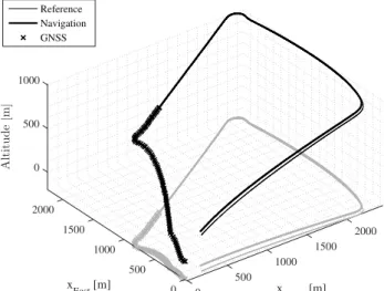
To evaluate the performance of the navigation system, a Monte Carlo simulation has been performed with 100 runs, using real 3D wind velocity data (KNMI and Alterra, 2012). While the tra-jectory and the wind has been kept the same in each realization, the error in observations, initialization, and VDM parameters has changed randomly for each individual run. Figure 3 depicts the reference trajectory, as well as the solution from a sample run.
For more comprehensible presentation, the results are presented in ENU frame, instead of navigation NED frame. The trajectory has a footprint bigger than2km×2kmon the ground and1km change in altitude. The results of Monte Carlo simulations are presented in sections 5.1 and 5.2.
0
2000 500
A
lt
it
u
d
e
[m
]
1000
1500 2000
x East [m]
1500 1000
x North [m] 1000 500
500
0 0
Reference Navigation GNSS
Figure 3: Reference trajectory and the solution from a sample rum with GNSS signals available during first100sonly
5.1 Navigation States
Figure 4 shows comparison of RMS of position and yaw errors for all the 100 runs between proposed VDM/INS/GNSS approach and classical INS/GNSS navigation algorithm over the whole in-terval. While the RMS of position error is11.7kmfor classical INS coasting after 5 minutes of autonomous navigation during GNSS outage, this is reduced to less than110mwith the pro-posed VDM/INS/GNSS integration under exactly the same situ-ations, which means an improvement of two orders of magnitude in position accuracy. The attitude determination also shows an improvement of 1 to 2 orders magnitude, which will be detailed shortly. It is worth mentioning here that the improved perfor-mance of the proposed filter is noticeable also during the avail-ability of GNSS in estimating yaw.
0 50 100 150 200 250 300 350 400
time [s] 0
2 4 6 8 10 12
P
o
si
ti
o
n
E
rr
o
r
[k
m
]
INS/GNSS Position Error (left y-axis) VDM/INS/GNSS Position Error INS/GNSS Yaw Error (right y-axis) VDM/INS/GNSS Yaw Error
0 3 6 9 12 15 18
A
tt
it
u
d
e
E
rr
o
r
[d
eg
]
GNSS Outage
Figure 4: Comparison between INS/GNSS and VDM/INS/GNSS: RMS of position and yaw errors from 100 Monte Carlo runs
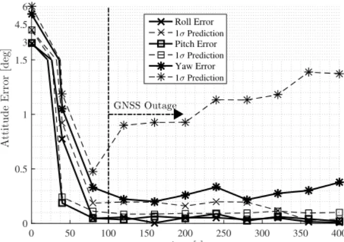
these individual errors and plotted against the predicted confi-dence level (1σ). It is important to notice that how closely (and slightly conservatively) the error is predicted within the filter, which reveals the correctness of filter setup.
0 50 100 150 200 250 300 350 400
time [s] 0
20 40 60 80 100 120 140 160
P
o
si
ti
o
n
E
rr
o
r
[m
]
GNSS Outage 100 runs RMS of Errors 1σ Prediction
Figure 5: Position errors for all the 100 Monte Carlo runs
Figure 6 depicts the empirical RMS of attitude errors for all the 100 runs, with associated predicted values of confidence (1σ). The results are very satisfactory in terms of preserved naviga-tion accuracy, with the RMS of error to be only0.0072◦ for roll,0.020◦for pitch, and0.38◦for yaw after 5 minutes of au-tonomous navigation during GNSS outage. In comparison, the classical INS coasting would result in errors of2.6◦for roll,1.5◦ for pitch, and16.6◦for yaw under exactly the same situations.
3 4.5 6
0 50 100 150 200 250 300 350 400
time [s] 0
0.5 1 1.5
A
tt
it
u
d
e
E
rr
o
r
[d
eg
]
GNSS Outage Roll Error 1σ Prediction Pitch Error 1σ Prediction Yaw Error 1σ Prediction
Figure 6: RMS of position and attitude errors from 100 Monte Carlo runs
5.2 Auxiliary States
Successful estimation of auxiliary states is a key enabler of navi-gation improvement within the filter. The results are briefly pre-sented in this section, with all the reported values calculated as an RMS of the values for all the 100 Monte-Carlo runs. More de-tailed results on auxiliary states estimation and associated plots are presented in (Khaghani and Skaloud, 2016).
The time correlated part of the IMU error gets estimated quickly during the first tens of seconds of navigation and remains rather unchanged afterwards, even during the GNSS outage period. The estimation error has an average of 6.0% for the three accelerom-eters and an average of 14.8% for the three gyroscopes at the end of the whole navigation period.
The mean error in estimation of VDM parameters shows a sharp decrease from the initial value of10%to6%during the first 40
seconds with GNSS available, which is followed by a slowly de-creasing trend until the end. The reason behind the second regime is the correlation between some parameters within the set. In such situations, the groups of parameters are estimated rather than dividual parameters, and those individual errors contribute to in-creasing the mean error for the whole set.
Finally, the wind velocity is estimated very well during GNSS availability period, reaching an error of only 3.9% for wind speed after 100 seconds. The estimation error starts to grow when GNSS outage begins. However, the rate of this growth is well controlled, and the error is still below 9.6% after 5 minutes of GNSS outage.
6. CONCLUSION
In this work, a novel method was presented to perform autonomous navigation and sensor integration for unmanned aerial vehicles. The key concept of this method is employing vehicle dynamic model in navigation system. Unlike the traditional method of kinematic modeling in which IMU serves as navigation process model within navigation filter, here the navigation filter features dynamic model of UAV as navigation process model whose out-put gets updated using IMU measurements. GNSS measurements can also be used within the filter whenever they are available, as well as other measurements such as those from a barometric al-timeter.
In addition to navigation states and error terms related to inertial sensors, UAV dynamic model parameters and wind velocity com-ponents can also be estimated within the filter. This is all possible with no extra sensors. The designed filter is thus polyvalent as it can accommodate changes in the platform and/or environmental conditions, such as the wind acting on the platform.
The scenario of GNSS signal reception disruption (e.g., due to electromagnetic interference) is a situation where this method can be most useful. In case of GNSS outage of 5 minutes, the pre-sented Monte Carlo simulations show an improvement of more than 2 orders of magnitudes in position accuracy compared to in-ertial coasting, for random initial errors of10%in UAV dynamic model parameters. Such gain of navigation autonomy is internal to UAV, therefore very suitable for limited or zero-visibility op-erations. Attitude estimation also shows a major improvement, reducing the error on yaw from16.61◦to only0.38◦for exam-ple. The parameters of the dynamic model are calibrated in flight and such calibration is possible even if GNSS signal reception is not available. The time-correlated errors in accelerometers and gyroscopes are also estimated within the filter as a random walk process, so are the wind velocity components.
Further development of current work will include studies on pro-posed navigation system in real scenarios. Technical and per-haps scientific challenges can be expected in real implementation. Proper time stamping of all sensor observations and scaling the control input signals are examples of technical challenges. On the scientific part, the main challenges will probably be related to unmodeled dynamics and disturbances, and the inclusion of addi-tional effects, such as sensor misalignments, actuator dynamics, UAV body elasticity, and asymmetric mass distribution.
ACKNOWLEDGEMENTS
REFERENCES
Angelino, C. V., Baraniello, V. R. and Cicala, L., 2012. UAV po-sition and attitude estimation using IMU, GNSS and camera. In: 15th International Conference on Information Fusion (FUSION), IEEE, pp. 735–742.
Bryson, M. and Sukkarieh, S., 2004. Vehicle model aided inertial navigation for a UAV using low-cost sensors. In: Proceedings of the Australasian Conference on Robotics and Automation, Cite-seer.
Bryson, M. and Sukkarieh, S., 2015. UAV Localization Using Inertial Sensors and Satellite Positioning Systems. In: Handbook of Unmanned Aerial Vehicles, Springer Netherlands, pp. 433– 460.
Cook, M. V., 2013. Flight dynamics principles a linear sys-tems approach to aircraft stability and control. Butterworth-Heinemann, Waltham, MA.
Crocoll, P. and Trommer, G. F., 2014. Quadrotor Inertial Nav-igation Aided by a Vehicle Dynamics Model with In-Flight Pa-rameter Estimation. In: Proceedings of the 27th International Technical Meeting of The Satellite Division of the Institute of Navigation (ION GNSS+ 2014), Tampa, Florida, pp. 1784–1795.
Crocoll, P., Seibold, J., Scholz, G. and Trommer, G. F., 2014. Model-Aided Navigation for a Quadrotor Helicopter: A Novel Navigation System and First Experimental Results. Navigation 61(4), pp. 253–271.
Dadkhah, N., Mettler, B. and Gebre-Egziabher, D., 2008. A model-aided ahrs for micro aerial vehicle application. In: Pro-ceedings of the 21st the International Technical Meeting of the Satellite Division of The Institute of Navigation ION GNSS 2008, pp. 545–553.
Ducard, G. J., 2009. Fault-tolerant flight control and guidance systems: Practical methods for small unmanned aerial vehicles. Springer, London.
Gelb, A. (ed.), 1974. Applied optimal estimation. M.I.T. Press, Cambridge, Massachusetts, London.
Groves, P. D., 2008. Principles of GNSS, inertial, and multisen-sor integrated navigation systems. GNSS technology and appli-cations series, Artech House, Boston.
Khaghani, M. and Skaloud, J., 2016. Autonomous Vehicle Dy-namic Model Based Navigation for Small UAVs. NAVIGATION, Journal of the Institute of Navigation (In Print).
KNMI and Alterra, 2012. Data provided by KNMI and Alterra, under the Consortium agreement on Cabauw Experimental Site for Atmospheric Research (CESAR), www.cesar-database.nl.
Koifman, M. and Bar-Itzhack, I. Y., 1999. Inertial navigation system aided by aircraft dynamics. IEEE Transactions on Control Systems Technology 7(4), pp. 487–493.
Lau, T. K., Liu, Y.-H. and Lin, K. W., 2013. Inertial-Based Localization for Unmanned Helicopters Against GNSS Outage. IEEE Transactions on Aerospace and Electronic Systems 49(3), pp. 1932–1949.
M¨uller, K., Crocoll, P. and Trommer, G., 2015. Wind Estimation for a Quadrotor Helicopter in a Model-Aided Navigation System. In: 22nd Saint Petersburg International Conference on Integrated Navigation Systems.
Noureldin, A., Karamat, T., Eberts, M. and El-Shafie, A., 2009. Performance Enhancement of MEMS-Based INS/GPS Integra-tion for Low-Cost NavigaIntegra-tion ApplicaIntegra-tions. IEEE TransacIntegra-tions on Vehicular Technology 58(3), pp. 1077–1096.
Schwarz, K. P. and Wei, M., 1994. Modeling INS/GPS for atti-tude and gravity applications. Proc. High Precision Navigation 95, pp. 200–18.
Sendobry, A., 2014. Control System Theoretic Approach to Model Based Navigation. Ingenieurwiss. Verlag, Bonn.
Vasconcelos, J., Silvestre, C., Oliveira, P. and Guerreiro, B., 2010. Embedded UAV model and LASER aiding techniques for inertial navigation systems. Control Engineering Practice 18(3), pp. 262–278.
Wang, J., Garratt, M., Lambert, A., Wang, J. J., Han, S. and Sin-clair, D., 2008. Integration of GPS/INS/vision sensors to navigate unmanned aerial vehicles. The International Archives of the Pho-togrammetry, Remote Sensing and Spatial Information Sciences 37, pp. 963–970.