Implementation of a 3-D-Var system for atmospheric profiling data assimilation into the RAMS model: initial results

(1)

AMTD

6, 3581–3610, 2013

Implementation of a 3-D-Var system for atmospheric profiling

data assimilation

S. Federico

Title Page

Abstract Introduction

Conclusions References

Tables Figures

◭ ◮

Back Close

Full Screen / Esc

Printer-friendly Version

Interactive Discussion

Discussion

P

a

per

|

Dis

cussion

P

a

per

|

Discussion

P

a

per

|

Discussio

n

P

a

per

|

Atmos. Meas. Tech. Discuss., 6, 3581–3610, 2013 www.atmos-meas-tech-discuss.net/6/3581/2013/ doi:10.5194/amtd-6-3581-2013

Atmospheric Measurement

Techniques

Open Access

Discussions

Geoscientiic Geoscientiic

This discussion paper is/has been under review for the journal Atmospheric Measurement Techniques (AMT). Please refer to the corresponding final paper in AMT if available.

Implementation of a 3-D-Var system for

atmospheric profiling data assimilation

into the RAMS model: initial results

S. Federico

ISAC-CNR, UOS of Rome, Rome (RM), Italy

Received: 3 March 2013 – Accepted: 29 March 2013 – Published: 12 April 2013

Correspondence to: S. Federico ([email protected])

Published by Copernicus Publications on behalf of the European Geosciences Union.

(2)

AMTD

6, 3581–3610, 2013

S. Federico

Title Page

Tables Figures

◭ ◮

Back Close

Full Screen / Esc

Discussion

P

a

per

|

Dis

cussion

P

a

per

|

Discussion

P

a

per

|

Discussio

n

P

a

per

|

Abstract

This paper presents the current status of development of a three-dimensional vari-ational data assimilation system. The system can be used with different numerical weather prediction models, but it is mainly designed to be coupled with the Regional At-mospheric Modelling System (RAMS). Analyses are given for the following parameters: 5

zonal and meridional wind components, temperature, relative humidity, and geopoten-tial height.

Important features of the data assimilation system are the use of incremental formu-lation of the cost-function, and the use of an analysis space represented by recursive filters and eigenmodes of the vertical background error matrix. This matrix and the 10

length-scale of the recursive filters are estimated by the National Meteorological Cen-ter (NMC) method.

The data assimilation and forecasting system is applied to the real context of atmo-spheric profiling data assimilation, and in particular to the short-term wind prediction. The analyses are produced at 20 km horizontal resolution over central Europe and 15

extend over the whole troposphere. Assimilated data are vertical soundings of wind, temperature, and relative humidity from radiosondes, and wind measurements of the European wind profiler network.

Results show the validity of the analysis solutions because they are closer to the observations (lower RMSE) compared to the background (higher RMSE), and the dif-20

ferences of the RMSEs are consistent with the data assimilation settings.

To quantify the impact of improved initial conditions on the short-term forecast, the analyses are used as initial conditions of a three-hours forecast of the RAMS model. In particular two sets of forecasts are produced: (a) the first uses the ECMWF analy-sis/forecast cycle as initial and boundary conditions; (b) the second uses the analyses 25

(3)

AMTD

6, 3581–3610, 2013

S. Federico

Title Page

Tables Figures

◭ ◮

Back Close

Full Screen / Esc

Discussion

P

a

per

|

Dis

cussion

P

a

per

|

Discussion

P

a

per

|

Discussio

n

P

a

per

|

The improvement is quantified by considering the horizontal components of the wind, which are measured at a-synoptic times by the European wind profiler network. The results show that the RMSE is effectively reduced at the short range (1–2 h). The results are in agreement with the set-up of the numerical experiment.

1 Introduction 5

Modern numerical weather prediction (NWP) data assimilation systems use information from a range of sources to provide the best estimate of the atmospheric state, i.e. the analysis, at a given time. These systems combine information coming from the observations, an a-priori estimate of the atmospheric state (the background or first-guess field), detailed error statistics, and the law of physics.

10

Nowadays, increased computing power coupled with greater access to real-time a-synoptic data is paving the way toward a new generation of high-resolution (i.e. on the order of 10 km or less) operational mesoscale analyses and forecast systems (Kalnay, 2003; Barker et al., 2003a; Lazarus, 2002). Moreover, better initial conditions are in-creasingly considered of the utmost importance for a range of NWP applications, in 15

particular at the short range (0–12 h, Zhang et al., 2005; Scenkman et al., 2011). The variational data assimilation systems have the advantage to assimilate quantities not trivially related to the standard atmospheric variables, as radiances, and they in-clude the imposition of dynamic balance either by the model itself (4-D-Var) or through the explicit use of balance equations. In recent years, these advantages have fos-20

tered the implementation of variational data assimilation systems in limited area mod-els (Barker et al., 2003a; Xiang-Yu et al., 2009; Zupanski et al., 2005). These systems replaced previously used scheme as, for example, optimal interpolation (Parrish and Derber, 1992; Rabier et al., 2000).

This paper shows the development of a three-dimensional stand-alone data assim-25

ilation system tailored to be used with the Regional Atmospheric Modeling System (RAMS; Cotton et al., 2003; Pielke, 2002). In particular, the data assimilation system

(4)

AMTD

6, 3581–3610, 2013

S. Federico

Title Page

Tables Figures

◭ ◮

Back Close

Full Screen / Esc

Discussion

P

a

per

|

Dis

cussion

P

a

per

|

Discussion

P

a

per

|

Discussio

n

P

a

per

|

can use the RAMS field as background and the analyses can be used to initialize the RAMS model.

The main features of the analysis system are:

1. Incremental formulation of the cost-function (Courtier et al., 1994), i.e. observa-tions are assimilated to provide analysis increments. In this way, the analysis im-5

balance is kept at minimum as the first guess, to which the increments are added, is already balanced because it comes from the output of a numerical model.

2. Preconditioning of the background cost function through a control variable trans-formation U defined as B=UUT, where B is the background error covariance matrix. Background error covariances are estimated by the Parrish and Derber 10

method (Parrish and Derber, 1992), also known as the National Meteorological Center (NMC) method.

3. Control variables are the two components of the horizontal wind, temperature and relative humidity. The geopotential height is retrieved from the increments of the horizontal wind through the geostrophic balance. This ensures the balance 15

between the mass and wind field increments. Moreover, the formulation permits to easily include more advanced balance equations in future implementations, as for example including the cyclostrophic flow and the friction. This will further extend the use of the data assimilation system in regions where the geostrophic balance is a poor approximation of the real atmospheric flow.

20

4. The horizontal component of the background error is represented through isotropic and homogeneous recursive filters. The vertical component of the back-ground error is represented through decomposition into climatologically averaged (in time, longitude and latitude) eigenvectors of the vertical error, which is com-puted by the NMC method.

25

(5)

AMTD

6, 3581–3610, 2013

S. Federico

Title Page

Tables Figures

◭ ◮

Back Close

Full Screen / Esc

Discussion

P

a

per

|

Dis

cussion

P

a

per

|

Discussion

P

a

per

|

Discussio

n

P

a

per

|

This paper presents an upgrade of the 2-D-Var data assimilation system reported in Federico (2013). Two important features are introduced: (a) the use of the 3-D-Var method, which replaces the 2-D-Var; (b) the option to run the analysis on the same horizontal coordinate system of the RAMS model, which simplifies the interaction be-tween the analysis and RAMS.

5

It is important to mention that a 4-D-Var data assimilation system is already in use for RAMS (Zupanski et al., 2005; Polkinghorne et al., 2009). Nevertheless the aim of this work is to realize a simple but e_ffective variational system, suitable for application and operational implementation in small meteorological centres. The 3-D-Var, indeed, requires less computational resources compared to 4-D-Var (Rabier et al., 2000) or 10

Ensemble Kalman filters (Anderson, 2001). It does not require the adjoint model and is simpler to implement. Moreover, the 3-D-Var system can be effective at improving the initial model state and has the advantages of variational data assimilation systems.

Even if the data assimilation system is continuously under development, it proves to be fast and reliable and can be used for real applications. So, while the basic aim 15

of the paper is to show the general characteristics of the 3-D-Var scheme, an appli-cation to the data assimilation of tropospheric profiles is given. It is also noticed that the numerical experiment set-up of this paper should be of interest for the atmospheric profiling community because it can be used in OSE (Observing System Experiment), which allows for the objective assessment and comparison of existing observing sys-20

tems, or in OSSE (Observing System Simulation Experiment), whose aim is to show the impact of next generation observing systems in a controlled software environment as, for example, weather prediction models (Otkin et al., 2011; Moninger et al., 2010).

The paper is divided as follows: Sect. 2 provides details about the data assimilation system; Sect. 3 shows the numerical experiment set-up; Sect. 4 gives the results of the 25

application to the short-term wind forecast, and Sect. 5 gives conclusions.

(6)

AMTD

6, 3581–3610, 2013

S. Federico

Title Page

Tables Figures

◭ ◮

Back Close

Full Screen / Esc

Discussion

P

a

per

|

Dis

cussion

P

a

per

|

Discussion

P

a

per

|

Discussio

n

P

a

per

|

2 The data assimilation system

The basic goal of the 3-D-Var algorithm is to produce an optimal estimate of the true at-mospheric state at analysis time through iterative solution of a prescribed cost-function (Ide et al., 1997):

J(x)=1

2(x−xb)

T_B−1_(x₋

x_b)+1

2(yo−H(x)) T

R−1(yo−H(x)) (1)

5

whereJ(x) is the cost-function,x is the state vector,x_bis the background state,H is the forward observational operator,y_o is the vector of the observations,B, and Rare the background, and observational error covariance matrices, respectively.

The problem can be summarized as the iterative solution of Eq. (1) to find the anal-ysis state x that minimizes J(x). This solution represents the a posteriori maximum 10

likelihood (minimum variance) estimate of the true state of the atmosphere given the two sources of a priori data: the backgroundx_band observationsy_o(Lorenc, 1986).

For a model state x with n∼106–107 degrees of freedom, the direct solution of Eq. (1) is practically unfeasible, because it requires ∼O(n2) calculations. One prac-tical implementation is to perform a preconditioning via a control variableχdefined by 15

x′=Uχ, wherex′=x−x_bis the model variable increment. The transformUis chosen to satisfy the relationshipB=UUT. Using the incremental formulation (Courtier et al., 1994) and the control variable transform, Eq. (1) may be rewritten:

J=1

2χ T

χ+1 2 y

′

o−HUχ T

R−1 y′_o−HUχ (2)

wherey′_o=y_o−H(x_b) is the innovation vector and H is the linearization of the poten-20

tially nonlinear observation operator H used in the calculation ofy′_o. In this form, the background term is diagonalized, reducing the number of calculations required from O(n2) toO(n).

(7)

AMTD

6, 3581–3610, 2013

S. Federico

Title Page

Tables Figures

◭ ◮

Back Close

Full Screen / Esc

Discussion

P

a

per

|

Dis

cussion

P

a

per

|

Discussion

P

a

per

|

Discussio

n

P

a

per

|

T′is the temperature increment. The model variable increment x′ is a vectorx′=(Z′, u′,v′, RH′, T′) where Z′ is a balanced geopotential height increment, and the other symbols are as inχ.

The transformx′=Uχfrom the control variableχto the model variable incrementx′ is implemented through three operators, namely Up,Uv, and Uh. The transform Up is 5

applied after the minimization of the cost function and will be discussed later on in this section; the implementation ofUvandUhfollows that of Barker et al. (2003a, b).

The transformUhis implemented by recursive filters (Purser et al., 2003). The recur-sive filter performs the task of convolving a spatial distribution of the innovations with a smoothing kernel, which is the covariance function of the background error. A single 10

pass of a recursive filter consists of an initial advancing smoothing:

F_i =(1−α)D_i+αF_i₋1

for increasing indexi, where D is the input forcing and F is the result of the sweep, followed by a backing sweep:

R_i =(1−α)F_i+αR_i₊1 15

For decreasingi, whereF is now the input and R is the response of the filter. The smoothing parameterα is between 0 and 1 and determines the correlation length of the smoothing response function.

The single-pass recursive filter of the operatorUh, involves one smoothing in the WE direction followed by one smoothing in the NS direction.

20

The recursive filter has two parameters: the number of passes and the length-scale d. The number of passes determines the response of the filter. In particular forN=2 the response approximates a second-order auto-regressive function (SOAR), while for N=∞ the response is Gaussian. In this paper twelve passes are used. This value ensures a well-shaped filter response, without the formation of unphysical lozenge-25

shaped model variable incrementx′.

(8)

AMTD

6, 3581–3610, 2013

S. Federico

Title Page

Tables Figures

◭ ◮

Back Close

Full Screen / Esc

Discussion

P

a

per

|

Dis

cussion

P

a

per

|

Discussion

P

a

per

|

Discussio

n

P

a

per

|

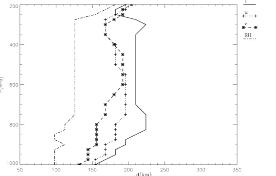
The length-scale of the recursive filters, which determines the smoothing parameter α(see Barker et al., 2003b for the details of the calculation), is computed by the NMC method (Parrish and Derber, 1992). This method gives a climatological estimate of the background error matrix by the averaged difference, computed over a sample, between two short-forecasts verifying at the same time. In this paper a one-month (July 2012) 5

series of 24 h minus 12 h forecasts verifying at 00:00 UTC of each day is used.

The length-scale in the model space is shown in Fig. 1. It depends on the height and on the variable, and it is larger for temperature and smaller for relative humidity. There is an evident increase of the length-scale above the Planetary Boundary Layer (PBL) for all variables. This is expected because the interaction between the orography 10

and the atmospheric flow in the PBL generates features smaller than those of the free atmosphere.

The vertical transform Uv is given by an empirical orthogonal function (EOF) de-composition of the vertical background error matrix (B_v). To determine B_v, the NMC method is applied, by averaging both is space (in longitude and latitude) and time the 15

difference series of 24 h minus 12 h forecasts valid at the same time (see Barker et al., 2003b for a detailed discussion). A one-month time series (July 2012) is used verifying at 00:00 UTC of each day. TheBvmatrix is symmetric and positive-defined and can be decomposed in the eigenvalues and eigenvector matrices, i.e.Bv=ELE

T

, where Eis the eigenvectors andL the eigenvalues matrix. Using this decomposition, the vertical 20

transformUv is written asUv=EL1/2.

To simplify the interpretation of the results, the error correlation between di_fferent variables is neglected in this paper and theUvmatrix is a block diagonal matrix, whose blocks are obtained by applying the above decomposition to each variable.

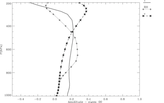
The leading eigenvector of the meridional wind component (Fig. 2), which describes 25

(9)

AMTD

6, 3581–3610, 2013

S. Federico

Title Page

Tables Figures

◭ ◮

Back Close

Full Screen / Esc

Discussion

P

a

per

|

Dis

cussion

P

a

per

|

Discussion

P

a

per

|

Discussio

n

P

a

per

|

main portion of the troposphere involved in wet processes in storms development. The temperature leading eigenvector, describing 48 % of the total variance, shows a rather constant profile in the troposphere, which is negatively correlated with errors in the upper troposphere. It should also be mentioned that the second leading eigenvector of temperature, which describe 26 % of the total variance, peaks at 900 hPa showing 5

a strong signal from errors in the planetary boundary layer.

After the minimization of the cost function, the physical transform Up is applied to transform the control variable χ=(u′, v′, RH′, T′) to the model variable increments x′=(Z′,u′,v′, RH′,T′), which differ only for the balanced geopotential increment.

The balanced geopotential increment is determined by the geostrophic equilibrium 10

in pressure coordinates (the analysis system uses pressure as vertical coordinate, see next section):

∇2pZ′= f ξ′

g (3)

where ξ′ is the vertical component of the relative potential vorticity computed from the increments of the zonal (u′) and meridional (v′) wind components,gis the gravity 15

(m s−2) andf is the Coriolis parameter (s−1).

The transform Up, ensures the balance between the mass and wind increments. A future development of the analysis scheme will involve the implementation of a more sophisticated balance equation improving the mass-wind balance in regions where the geostrophic balance is a coarse approximation of the real flow, as the tropics or the 20

PBL.

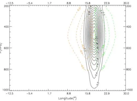
Figure 3 shows the combined effect of the transformsUp,Uv and Uh. In particular it is shown the longitude-height cross section at 57◦N latitude for the meridional velocity increment and for the geopotential height increment determined by a single meridional wind component observation introduced over the Gotland Island∼(57.5◦N, 18◦E) at 25

500 hPa. The final increment is spread vertically by theUv transform and horizontally byUh. TheUptransform determines the increment of the geopotential height.

(10)

AMTD

6, 3581–3610, 2013

S. Federico

Title Page

Tables Figures

◭ ◮

Back Close

Full Screen / Esc

Discussion

P

a

per

|

Dis

cussion

P

a

per

|

Discussion

P

a

per

|

Discussio

n

P

a

per

|

Before concluding this section it is important to consider the observation and back-ground errors (σ_b2, σo2), which determine the relative weight given to the background and observations in the analysis scheme. It is assumed that the observational errors are uncorrelated with each other, so the matrixRin Eq. (2) is a diagonal matrix whose elements are all equal to σo2. The dimensions of the matrix R equals the number of 5

measurements available at the analysis time. The value ofσo2is taken from the bibliog-raphy (Lazarus et al., 2002; Sashegyi et al., 1993) and it is shown in Federico (2013). More in detail, the observational error is equal for the zonal and meridional wind compo-nents. It increases from 2.5 m s−1at 1000 hPa to 4 m s−1at 300 hPa. Then it decreases to 3.5 m s−1 at 200 hPa. Above 200 hPa the observational error for the velocity compo-10

nents is held constant. For the relative humidity, the observational error is held constant (10 %) from 1000 hPa to 500 hPa, then it increases to 20 % at 200 hPa. Above 200 hPa the relative humidity is not assimilated. For the temperature, the observational error decreases from 1.8 K at 1000 hPa to 1.0 K at 800 hPa. Then it is held constant up to 500 hPa. The error increases from 1.0 K to 2.0 K between 500 and 300 hPa, and is held 15

constant above this level.

The background error is twice the observational error, i.e.σ_b2=2σo2 for all variables and for all levels. So, it is assumed that the background is less reliable than observa-tions.

3 The experiment set-up 20

The background and the forecast are issued by the RAMS model (non-hydrostatic), version 6.0. Its physical settings are summarized in Table 1.

The strategy to show the impact of the data assimilation on the analysis and short-term forecast is similar to Federico (2013). However, for the paper readability, most of the discussion is repeated in this section.

25

(11)

AMTD

6, 3581–3610, 2013

S. Federico

Title Page

Tables Figures

◭ ◮

Back Close

Full Screen / Esc

Discussion

P

a

per

|

Dis

cussion

P

a

per

|

Discussion

P

a

per

|

Discussio

n

P

a

per

|

uses a rotated polar stereographic projection, whose pole is near the centre of the do-main to minimize the projection distortion (Pielke, 2002). In the vertical direction, RAMS uses the sigma-z terrain following coordinate (Pielke, 2002), while the analysis uses pressure.

The possibility to run the analysis on the same horizontal coordinate system of 5

RAMS, eventually with coarsened horizontal resolution to speed-up the analysis, is an important feature. Indeed, in the former set-up, the analysis was performed on a regularly-spaced latitude-longitude grid, whose domain was contained in the domain of the RAMS forecast, which was referred as background run. The analysis was used to initialize a RAMS simulation, referred as forecast-run, whose domain was contained 10

in the analysis domain. This process required two di_fferent RAMS set-up for the back-ground and forecast run. The new added feature requires one RAMS configuration only and simplifies the interpolation between the RAMS and analysis grids1.

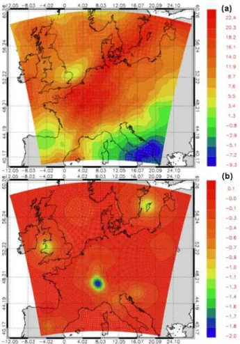
Figure 4 shows an analysis example for the zonal wind component. The background has 10 km horizontal resolution and covers the central Europe. Its grid setting is shown 15

in Table 2. The analysis increments are given on the same grid as the background but with halved horizontal resolution (20 km) to speed-up the analysis computation.

RAMS uses thirty-three levels in the vertical. The analysis grid uses twenty-nine pressure levels from 1000 hPa to 50 hPa, spaced every 50 hPa between 800 and 300 hPa, and every 25 hPa below 800 hPa. Above 300 hPa the vertical levels are un-20

evenly spaced with a maximum distance of 25 hPa.

Observations used in this paper are upper-air soundings (both land and ship) inside the analysis domain, and the European wind profiler network. Upper-air soundings re-ports contain vertical profiles of temperature, relative humidity, wind speed and direc-tion, and pressure and are available at synoptic hours (00:00, 06:00, 12:00, 18:00 UTC) 25

1

The option to run the analysis on a regularly spaced longitude-latitude grid is still avail-able to use the ISAN (ISentropic Analysis) package, which is the standard method to initialize RAMS (see the RAMS technical manual available at http://www.atmet.com/html/docs/rams/ rams techman.pdf).

(12)

AMTD

6, 3581–3610, 2013

S. Federico

Title Page

Tables Figures

◭ ◮

Back Close

Full Screen / Esc

Discussion

P

a

per

|

Dis

cussion

P

a

per

|

Discussion

P

a

per

|

Discussio

n

P

a

per

|

with few exceptions. The European wind profilers network measures the wind speed and direction in the vertical above the instrument and observations are available every one-hour.

Observations were downloaded from the MARS (Meteorological Archive and Re-trieval System, see also http://www.ecmwf.int/publications/manuals/mars/) archive of 5

ECMWF (European Centre for Medium Weather range Forecast) and the numerical experiment is performed for the month of July 2012. A quality check of the measure-ments is performed to discard observations a_ffected by gross errors. In particular, only observations whose difference with the background is under a fixed threshold are used in the analyses. The thresholds considered in this paper are equal for all levels and are 10

the following: 8 m s−1 for zonal and meridional wind components, 4 K for temperature and 20 % for relative humidity. The application of this quality check discarded less than 5 % of the observations for all variables.

To quantify the impact of the analysis both on the improvement of the initial state and on the short-term forecast, the following strategy is adopted (Fig. 5). For each day 15

of July 2012 one background run lasting 24 h is made starting at 00:00 UTC. Its initial and boundary conditions are taken, every 6 h, from the 00:00 UTC operational analy-sis/forecast cycle of ECMWF. These fields are available at 0.25◦horizontal resolution.

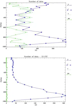
After 12 h of each run, an analysis is made. The 12:00 UTC was chosen because there are several upper-air soundings and wind profiler reports. Figure 6a shows the 20

number of data available for the analyses for the whole period, while Fig. 4b gives an idea of the distribution of the data inside the domain at an analysis time. It is notice-able that there are more data for the wind components because of the data from the European wind profiler network.

Starting from the analysis time (12:00 UTC), a short-term RAMS forecast, lasting 3 h, 25

(13)

AMTD

6, 3581–3610, 2013

S. Federico

Title Page

Tables Figures

◭ ◮

Back Close

Full Screen / Esc

Discussion

P

a

per

|

Dis

cussion

P

a

per

|

Discussion

P

a

per

|

Discussio

n

P

a

per

|

The comparison of these statistics at the analysis time shows the performance of the data assimilation system; the same comparison for times following the analysis time quantifies the impact of the analyses on the short-term forecast.

Statistics are presented for the zonal and meridional wind components only, because few data are available for other variables after the analysis time. Indeed, temperature 5

and relative humidity, which are measured by upper-air soundings, are available at syn-optic times (00:00, 06:00, 12:00, 18:00 UTC) with few exceptions, while wind observa-tions are available every one-hour by wind profiler measurements. For example, Fig. 6b shows the number of data at 13:00 UTC for the whole period. Less than 5 observations are available for temperature and relative humidity at all levels, while the number of 10

data for the wind components varies from 309 (875 hPa) to 25 (130 hPa). From Fig. 6 it is apparent that statistics for temperature and relative humidity are reliable only at the analysis time and they will be shortly discussed in the next section.

4 Results

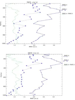
Hereafter the RMSE computed between the background run and the observations at 15

a fixed time and for the whole period is referred as the background error (RMSE b). Similarly, the RMSE computed between the forecast run and the observations at a fixed time and for the whole period is referred as the forecast error (RMSE f). For the com-putation of both RMSEs, the grid point nearest to the observation is considered and the statistics are computed for the whole domain (Fig. 4).

20

It should also be emphasized that RMSE f at the analysis time is computed after the analyses have been used to initialize the RAMS model. So, the difference between the RMSE b and RMSE f accounts for the errors introduced by the vertical interpolation between the RAMS and analysis grids.

Figure 7a shows the RMSE for the zonal wind component. The RMSE b is about 25

2.0 m s−1 up to 500 hPa, while it increases above this level reaching a maximum of

(14)

AMTD

6, 3581–3610, 2013

S. Federico

Title Page

Tables Figures

◭ ◮

Back Close

Full Screen / Esc

Discussion

P

a

per

|

Dis

cussion

P

a

per

|

Discussion

P

a

per

|

Discussio

n

P

a

per

|

3.4 m s−1 at 250 hPa. The forecast error at the analysis time (RMSE f) decreases by more than 1.0 m s−1for most levels and RMSE f is more than halved below 900 hPa.

Similar considerations apply for the meridional wind component (Fig. 7b), whose RMSE f is ∼1.0 m s−1 lower than RMSE b for most levels; moreover below 850 hPa the error is more than halved.

5

For the other parameters (not shown, see Federico, 2013) similar results are ob-tained, with a significant reduction of the error at the analysis time (30–60 % of the background error). The improvement is comparatively larger at the lower levels.

Even if it is not simple to quantify the performance of the data assimilation scheme because the performance varies with the parameter and with the height, a discussion 10

is provided to clarify the results of Fig. 7.

First it should be noticed that the analyses e_ffectively reduce the error. The analy-sis RMSE is lowered by 30–50 % of the background value for most levels and for all parameters; for few levels, the RMSE reduction is larger than 50 % of the background value.

15

The error reduction of 30–50 % of the background value is in reasonable agreement with the setting of the data assimilation system. In particular, considering that the model errorσ_b2 is twice the observational errorσo2at all levels, and for the ideal case of one measurement available at a grid point of the analysis grid, the analysis at this point is closer to the observation than to the background, and the error is more than halved. In 20

particular, for this simple ideal case it can be shown that the analysis error (RMSE f) is σo2/(σ

2 o+σ

2

b) of the background error (RMSE b; Kalnay, 2003), with an error reduction of 67 %.

The limit of this simple ideal case is not attained in the application of the analysis system for two main reasons: (a) the difference between RMSE f and RMSE b of Fig. 7 25

(15)

AMTD

6, 3581–3610, 2013

S. Federico

Title Page

Tables Figures

◭ ◮

Back Close

Full Screen / Esc

Discussion

P

a

per

|

Dis

cussion

P

a

per

|

Discussion

P

a

per

|

Discussio

n

P

a

per

|

observations, interact with each other, as shown by the analysis increments in Northern Italy and Swiss of Fig. 4b.

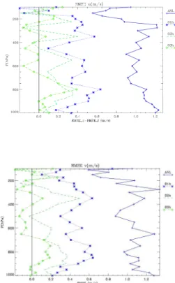
It is interesting to consider the impact of the analysis on the short-term forecast. Figure 8 shows the difference between RMSE b and RMSE f for the wind compo-nents. A positive difference means that the short-term forecast has a lower error than 5

the background and the wind forecast is effectively improved by using the analyses as initial conditions.

After one hour forecast, the improvement of the performance for the zonal velocity is apparent. In particular, the difference of the RMSE b and RMSE f is positive for all levels but 150 and 110 hPa and it is larger than 0.4 m s−1 for several levels. A useful 10

statistic to represent the impact of the analysis on the short-term forecast is the ver-tically averaged value of the difference between RMSE b and RMSE f. This value is 1.00 m s−1 for the analysis time and 0.35 m s−1 for the one-hour forecast. From these values it follows that the use of the analyses effectively reduces the error (35 % of the value at the analysis time) after one-hour forecast.

15

After two-hours forecast the improvement reduces. The vertical average of the diff er-ence between RMSE b and RMSE f is 0.15 m s−1, showing that the improvement after two-hours forecast is a sizeable fraction, i.e. larger than 10 %, of the initial value, and that the analysis is still effective at improving the short-term forecast.

For the three-hours forecast the impact of the analysis on the short-term forecast 20

is negligible in practice. There are several levels for which the di_fference between RMSE b and RMSE f is negative, and its vertical average is 0.04 m s−1.

Figure 8b shows the same statistics of Fig. 8a for the meridional wind component. The impact of the analysis on the one-hour forecast reduces the error of 0.1–0.6 m s−1, depending on the level. The improvement after one-hour forecast is slightly better for 25

the meridional wind component compared to the zonal wind component. This is con-firmed by the vertical average of the di_fference between RMSE b and RMSE f, which is 0.45 m s−1. This value must be compared with 1.03 m s−1 at the analysis time, and shows a positive impact of the analysis on the one-hour forecast.

(16)

AMTD

6, 3581–3610, 2013

S. Federico

Title Page

Tables Figures

◭ ◮

Back Close

Full Screen / Esc

Discussion

P

a

per

|

Dis

cussion

P

a

per

|

Discussion

P

a

per

|

Discussio

n

P

a

per

|

After two-hours, the improvement is reduced, nevertheless its value is larger than 0.2 m s−1 for several levels. The vertical average of the di_fference between RMSE b and RMSE f is 0.16 m s−1, which is still a sizeable fraction (16 %) of its initial value.

After three-hours forecast, the improvement is negligible (2 % of the initial value con-sidering the vertical average of the di_fference between RMSE b and RMSE f), and 5

several levels shows a negative impact of the analysis on the short-term forecast. From the above results, it can be concluded that, for the setting of this paper, the use of the analysis has a positive impact on the one-hour and two-hours forecast for both wind components.

This result is encouraging because the number of data used in the analysis is small. 10

Moreover, it is in agreement with the numerical experiment settings. Indeed, consider-ing the wind components, which have the largest number of measurements, the num-ber of data used by the analysis is, on average, less than 10 for most levels (Fig. 6a). The corrections introduced by these measurements through the analyses, i.e. the anal-ysis increments, are centred at the observational point and have a radius of influence 15

that depends on height, but which is of the order of 100 km (Fig. 1). The analysis incre-ments are advected downwind of the measurement point in few hours, in agreement with the results of this section. It is expected that, using a larger number of data, the positive impact of the analysis on the short-term forecast would last longer.

5 Conclusions 20

This paper presents the current state of development of a 3-D-Var analysis system, tailored for the RAMS model, which is computationally fast and can be used in small meteorological centres.

The cost-function is written in the incremental form, which ensures that unbalances introduced by the analysis increments are kept at minimum. For the practical minimiza-25

(17)

AMTD

6, 3581–3610, 2013

S. Federico

Title Page

Tables Figures

◭ ◮

Back Close

Full Screen / Esc

Discussion

P

a

per

|

Dis

cussion

P

a

per

|

Discussion

P

a

per

|

Discussio

n

P

a

per

|

transforms applied in sequence: the horizontal transformUh, and the vertical transform Uv.

The horizontal transform Uh is applied through recursive filters, which are compu-tationally fast, while the vertical transform Uv is obtained through the eigenvalues-eigenvectors decomposition of the vertical component of the background error matrix. 5

The length-scale of the recursive filters and the vertical component of the background error matrix are estimated by the NMC method.

The increment of the geopotential height is computed after the minimization of the cost-function, by applying the geostrophic balance to the wind increments (Up trans-form). This ensures the balance between the increments of the mass and wind fields. 10

A practical example is shown for the analysis/short-term wind forecast (0–3 h). Anal-yses are produced once a day at 12:00 UTC for July 2012 with a horizontal resolution of 20 km and twenty-nine vertical levels. Observations are tropospheric profiles of wind, temperature and relative humidity from upper-air soundings, and tropospheric wind profiles from the European wind profiler network.

15

Analyses are effective at reducing the initial model error. The improvement is be-tween 30 % and 60 % of the background error for all parameters for most levels. It was shown that this improvement is in agreement with the data assimilation setting, never-theless there is a decrease of the performance with increasing height caused by the errors introduced by the vertical interpolation between the RAMS and analysis grids. 20

The impact of the analyses on the short-term forecast is evaluated for the wind com-ponents only, because there are few measurements for other variables.

The results show that the improvement for the one-hour forecast is larger than 30 % of the error reduction at the analysis time for both wind components. The same im-provement is larger than 15 % of the error reduction at the analysis time for the two-25

hours forecast and for both wind components. The (positive) impact of the analysis after three-hours forecast is negligible in practice.

(18)

AMTD

6, 3581–3610, 2013

S. Federico

Title Page

Tables Figures

◭ ◮

Back Close

Full Screen / Esc

Discussion

P

a

per

|

Dis

cussion

P

a

per

|

Discussion

P

a

per

|

Discussio

n

P

a

per

|

It is concluded that, considering the amount of data used in the data assimilation, the results are encouraging and are in agreement with the set-up of the numerical experiment.

Work is in progress on several aspects of the data assimilation system. In particular, future development will consider the inclusion of measurements coming from di_fferent 5

sources and a more sophisticated balance for theUptransform. Nevertheless, the anal-ysis system and the numerical experiment presented in this work should be of interest for the atmospheric profiling community because it can be applied to OSE and OSSE experiments.

Acknowledgements. Most of the elaborations of this work were performed on the ECMWF

10

supercomputing environment, in the framework of the special project SPITFEDE. I am grateful to the “Aereonautica Militare Italiana” and to the ECMWF for the data and for their support in using the MARS archive.

References

Anderson, J.: An ensemble adjustment Kalman filter for data assimilation, Mon. Weather Rev., 15

129, 2884–2903, 2001.

Barker, D. M., Huang, W., Guo, Y.-R., and Xiao, Q. N.: A three-dimensional variational data assimilation system for MM5: implementation and initial results, Mon. Weather Rev., 132, 897–914, 2003a.

Barker, D. M., Huang, W., Guo, Y.-R., and Bourgeois, A.: A three-dimensional variational (3-20

DVAR) data assimilation system for use with MM5, NCAR Tech. Note. NCAR/TN-453 1 STR, 68 pp., available from UCAR Communications, P.O. Box 3000, Boulder, CO 80307, 2003b.

Chen, C. and Cotton, W. R.: A one-dimensional simulation of the stratocumulus-capped mixed layer, Bound.-Lay. Meteorol., 25, 289–321, 1983.

25

(19)

AMTD

6, 3581–3610, 2013

S. Federico

Title Page

Tables Figures

◭ ◮

Back Close

Full Screen / Esc

Discussion

P

a

per

|

Dis

cussion

P

a

per

|

Discussion

P

a

per

|

Discussio

n

P

a

per

|

Courtier, P., Th ´epaut, J. N., and Hollingsworth, A.: A strategy for operational implementation of 4-D-Var, using an incremental approach, Q. J. Roy. Meteor. Soc., 120, 1367–1387, 1994. Federico, S.: Preliminary results of a data assimilation system, Atmos. Climate Sci., 3, 61–72,

2013.

Kalnay, E.: Atmospheric Modeling, Data Assimilation and Predictability, Cambridge University 5

Press, Cambridge, UK, 2003.

Ide, K., Courtier, P., Ghil, M., and Lorenc, A. C.: Unified notation for data assimilation: opera-tional, sequential and variaopera-tional, J. Meteorol. Soc. Jpn., 75, 181–189, 1997.

Lazarus, S. M, Ciliberti, C. M., Horel, J. D., and Brewster, K. A.: Near-real-time applications of a mesoscale analysis system to complex terrain, Weather Forecast., 17, 149–160, 2002. 10

Lorenc, A. C.: Analysis methods for numerical weather prediction, Q. J. Roy. Meteor. Soc., 112, 1177–1194, 1986.

Mellor, G. and Yamada, T.: Development of a turbulence closure model for geophysical fluid problems, Rev. Geophys. Space Ge., 20, 851–875, 1982.

Molinari, J. and Corsetti, T.: Incorporation of cloud-scale and mesoscale down-drafts into a cu-15

mulus parametrization: results of one and three-dimensional integrations, Mon. Weather Rev., 113, 485–501, 1985.

Moninger, W. R., Benjamin, S. G., Jamison, B. D., Schlatter, T. W., Smith, T. L., and Szoke, E. D.: Evaluation of regional aircraft observations using TAMDAR, Weather Forecast., 25, 627–645, 2010.

20

Otkin, J. A., Hartung, D. C., Turner, D. D., Petersen, R. A., Feltz, W. F., and Janzon, E., Assimilation of surface-based boundary layer profiler observations during a cool-season weather event using an observing system simulation experiment. Part I: analysis impact, Mon. Weather Rev., 139, 2327–2346, 2011.

Parrish, D. F. and Derber, J. C.: The National Meteorological Center’s spectral statistical inter-25

polation analysis system, Mon. Weather Rev., 120, 1747–1763, 1992.

Pielke, R. A: Mesoscale Meteorological Modeling, Academic Press, San Diego, 2002.

Polkinghorne, R., Vukicevic, T., and Evans, K. F.: Validation of cloud-resolving model back-ground data for cloud data assimilation, Mon. Weather Rev., 138, 781–795, 2009.

Press, W. H., Teukolsky, S. A., Vetterling, W. T., and Flannery, B. P.: Numerical Recipes in 30

Fortran 77, second edn., Cambridge University Press, Cambridge, 1446 pp., 1992.

(20)

AMTD

6, 3581–3610, 2013

S. Federico

Title Page

Tables Figures

◭ ◮

Back Close

Full Screen / Esc

Discussion

P

a

per

|

Dis

cussion

P

a

per

|

Discussion

P

a

per

|

Discussio

n

P

a

per

|

Purser, R. J., Wu, W.-S., Parrish, D. F., and Roberts, N. M.: Numerical aspects of the applica-tion of recursive filters to variaapplica-tional statistical analysis. Part I: spatially homogeneous and isotropic Gaussian covariances, Mon. Weather Rev., 131, 1524–1535, 2003.

Rabier, F., J ¨arvinnen, H., Klinker, E., Mahfouf, J.-F., and Simmons, A.: The ECMWF operational implementation of four-dimensional variational assimilation. I: experimental results with sim-5

plified physics, Q. J. Roy. Meteor. Soc., 126, 1143–1170, 2000.

Sashegyi, D. K., Harms, D. E., Madala, R. V., and Raman, S.: Application of the Bratseth scheme for the analysis of GALE, data using a mesoscale model, Mon. Weather Rev., 121, 207–220, 1993.

Schenkman, A. D., Xue, M., Shapiro, A., Brewster, K., and Gao, J.: The analysis and prediction 10

of the 8–9 May 2007 oklahoma tornadic mesoscale convective system by assimilating WSR-88D and CASA radar data using 3-DVAR, Mon. Weather Rev., 139, 224–246, 2011.

Smagorinsky, J.: General circulation experiments with the primitive equations. Part I, the basic experiment, Mon. Weather Rev., 91, 99–164, 1963.

Walko, R. L., Cotton, W. R., Meyers, M. P., and Harrington, J. Y.: New RAMS cloud microphysics 15

parameterization part I: the single-moment scheme, Atmos. Res., 38, 29–62, 1995.

Walko, R. L., Band, L. E., Baron, J., Kittel, T. G., Lammers, R., Lee, T. J., Ojima, D., Pielke, R. A. Sr., Taylor, C., Tague, C., Tremback, C. J., and Vidale, P. L.: Coupled atmosphere-biosphere-hydrology models for environmental prediction, J. Appl. Met., 39, 931–944, 2000.

Xiang-Yu, H., Qingnong, X., Barker, D. M., Zhang, X., Michalakes, J., Huang, W., Henderson, T., 20

Bray, J., Chen, Y., Ma, Z., Dudhia, J., Guo, Y., Zhang, X., Won, D. J., Lin, H. C., and Kuo, Y. H.: Four-dimensional variational data assimilation for WRF: formulation and preliminary results, Mon. Weather Rev., 137, 299–314, doi:10.1175/2008MWR2577.1, 2009.

Zhang, F., Meng., Z., and Askoy, A.: Tests of an ensemble Kalman filter for mesoscale and regional-scale data assimilation. Part I: perfect model experiments, Mon. Weather Rev., 134, 25

722–736, 2005.

(21)

AMTD

6, 3581–3610, 2013

S. Federico

Title Page

Tables Figures

◭ ◮

Back Close

Full Screen / Esc

Discussion

P

a

per

|

Dis

cussion

P

a

per

|

Discussion

P

a

per

|

Discussio

n

P

a

per

|

Table 1.RAMS model physical settings.

Physical option Description

Parametrized Modified Kuo scheme to account for updraft and downdraft cumulus convection (Molinari and Corsetti, 1985).

Explicit precipitation Bulk microphysical model which prognoses cloud water, parametrization rain, snow, pristine ice, graupel and hail (Walko et al., 1995).

Subgrid mixing The turbulent mixing in the horizontal directions is

parameterized following Smagorinsky (1963), which relates the mixing coefficients to the fluid strain rate and

includes corrections for the influence of the Brunt-Vaisala frequency and the Richardson number (Pielke, 2002). Vertical diffusion is parameterized according to the Mellor and Yamada (1982) scheme, which employs a prognostic turbulent kinetic energy.

Exchange between LEAF-3 sub-model (Walko et al., 2000). LEAF includes prognostic the surface, the equations for soil temperature and moisture for multiple layers, biosphere and the vegetation temperature and surface water including dew and atmosphere. intercepted rainfall, snow cover mass and thermal energy for

multiple layers, and temperature and water vapour mixing ratio of canopy air.

Radiation scheme A full-column, two-stream single-band radiation scheme is used to calculate short-wave and long-wave radiation (Chen and Cotton, 1983). The Chen and Cotton scheme accounts for condensate in the atmosphere, but not for specific optical properties of ice

hydrometeors.

(22)

AMTD

6, 3581–3610, 2013

S. Federico

Title Page

Tables Figures

◭ ◮

Back Close

Full Screen / Esc

Discussion

P

a

per

|

Dis

cussion

P

a

per

|

Discussion

P

a

per

|

Discussio

n

P

a

per

|

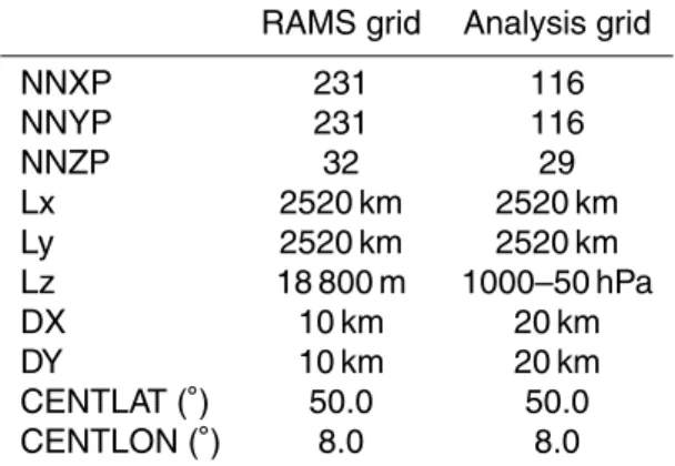
Table 2.RAMS and analysis grid-settings. NNXP, NNYP and NNYZ are the number of grid points in the west-east, north-south, and vertical directions. Lx (km), Ly (km), Lz (m) are the domain extension in the west-east, north-south, and vertical directions. DX (km) and DY (km) are the horizontal grid resolutions in the west-east and north-south directions. CENTLON and CENTLAT are the geographical coordinates of the grid centres. The analysis grid uses pressure as vertical coordinate.

RAMS grid Analysis grid

NNXP 231 116

NNYP 231 116

NNZP 32 29

Lx 2520 km 2520 km Ly 2520 km 2520 km Lz 18 800 m 1000–50 hPa

DX 10 km 20 km

DY 10 km 20 km

(23)

AMTD

6, 3581–3610, 2013

S. Federico

Title Page

Tables Figures

◭ ◮

Back Close

Full Screen / Esc

Discussion

P

a

per

|

Dis

cussion

P

a

per

|

Discussion

P

a

per

|

Discussio

n

P

a

per

|

Fig. 1. Length-scale of the different parameters of the control variable as a function of the pressure.uis for zonal velocity,v is for meridional velocity,T is for temperature, and RH is for relative humidity.

(24)

AMTD

6, 3581–3610, 2013

S. Federico

Title Page

Tables Figures

◭ ◮

Back Close

Full Screen / Esc

Discussion

P

a

per

|

Dis

cussion

P

a

per

|

Discussion

P

a

per

|

Discussio

n

P

a

per

|

(25)

AMTD

6, 3581–3610, 2013

S. Federico

Title Page

Tables Figures

◭ ◮

Back Close

Full Screen / Esc

Discussion

P

a

per

|

Dis

cussion

P

a

per

|

Discussion

P

a

per

|

Discussio

n

P

a

per

|

Fig. 3.The effect of theUh,UvandUptransforms (see text for details). Solid lines are contours

of meridional wind increments (v′, contours from₋2.4 to₋0.2 m s−1with 0.2 interval); dashed lines are the geopotential height incrementsZ′ (negative to the East and positive to the West of the observation position, contours from₋1.0 to 1.0 m with 0.2 m interval).

(26)

AMTD

6, 3581–3610, 2013

S. Federico

Title Page

Tables Figures

◭ ◮

Back Close

Full Screen / Esc

Discussion

P

a

per

|

Dis

cussion

P

a

per

|

Discussion

P

a

per

|

Discussio

n

P

a

per

|

(27)

AMTD

6, 3581–3610, 2013

S. Federico

Title Page

Tables Figures

◭ ◮

Back Close

Full Screen / Esc

Discussion

P

a

per

|

Dis

cussion

P

a

per

|

Discussion

P

a

per

|

Discussio

n

P

a

per

|

Fig. 5.Synopsis of the simulations. BCKG is the background run, which lasts 24 h. ANL is the analysis time: an analysis is performed at 12:00 UTC. FCST is the short-term forecast, which lasts 3 h.

(28)

AMTD

6, 3581–3610, 2013

S. Federico

Title Page

Tables Figures

◭ ◮

Back Close

Full Screen / Esc

Discussion

P

a

per

|

Dis

cussion

P

a

per

|

Discussion

P

a

per

|

Discussio

n

P

a

per

|

(29)

AMTD

6, 3581–3610, 2013

S. Federico

Title Page

Tables Figures

◭ ◮

Back Close

Full Screen / Esc

Discussion

P

a

per

|

Dis

cussion

P

a

per

|

Discussion

P

a

per

|

Discussio

n

P

a

per

|

Fig. 7.RMSE of the background field (RMSE b), of the analyses (RMSE f), and their difference (RMSE b-RMSE f) for:(a)zonal wind component;(b)meridional wind component. The RMSEs are computed for the whole period considering the grid-points nearest to the observations. The RMSE f statistics are computed after the RAMS model has been initialized by the analyses.

(30)

AMTD

6, 3581–3610, 2013

S. Federico

Title Page

Tables Figures

◭ ◮

Back Close

Full Screen / Esc

Discussion

P

a

per

|

Dis

cussion

P

a

per

|

Discussion

P

a

per

|

Discussio

n

P

a

per

|