Spike Time Correlations
James Trousdale1*, Yu Hu2, Eric Shea-Brown2, Kresˇimir Josic´1,3
1Department of Mathematics, University of Houston, Houston, Texas, United States of America,2Department of Applied Mathematics, Program in Neurobiology and Behavior, University of Washington, Seattle, Washington, United States of America,3Department of Biology and Biochemistry, University of Houston, Houston, Texas, United States of America
Abstract
Novel experimental techniques reveal the simultaneous activity of larger and larger numbers of neurons. As a result there is increasing interest in the structure of cooperative – orcorrelated– activity in neural populations, and in the possible impact of such correlations on the neural code. A fundamental theoretical challenge is to understand how the architecture of network connectivity along with the dynamical properties of single cells shape the magnitude and timescale of correlations. We provide a general approach to this problem by extending prior techniques based onlinear response theory. We consider networks of general integrate-and-fire cells with arbitrary architecture, and provide explicit expressions for the approximate cross-correlation between constituent cells. These correlations depend strongly on the operating point (input mean and variance) of the neurons, even when connectivity is fixed. Moreover, the approximations admit an expansion in powers of the matrices that describe the network architecture. This expansion can be readily interpreted in terms of paths between different cells. We apply our results to large excitatory-inhibitory networks, and demonstrate first how precisebalance– or lack thereof – between the strengths and timescales of excitatory and inhibitory synapses is reflected in the overall correlation structure of the network. We then derive explicit expressions for the average correlation structure in randomly connected networks. These expressions help to identify the important factors that shape coordinated neural activity in such networks.
Citation:Trousdale J, Hu Y, Shea-Brown E, Josic´ K (2012) Impact of Network Structure and Cellular Response on Spike Time Correlations. PLoS Comput Biol 8(3): e1002408. doi:10.1371/journal.pcbi.1002408
Editor:Olaf Sporns, Indiana University, United States of America
ReceivedOctober 21, 2011;AcceptedJanuary 11, 2012;PublishedMarch 22, 2012
Copyright:ß2012 Trousdale et al. This is an open-access article distributed under the terms of the Creative Commons Attribution License, which permits unrestricted use, distribution, and reproduction in any medium, provided the original author and source are credited.
Funding:This work was supported by NSF grants 0817649, 1122094, and a Texas ARP/ATP award to KJ, as well as NSF Grants 1122106, DMS-0818153, and a Burroughs Wellcome Career Award at the Scientic Interface to ESB. The funders had no role in study design, data collection and analysis, decision to publish, or preparation of the manuscript.
Competing Interests:The authors have declared that no competing interests exist. * E-mail: [email protected]
Introduction
New multielectrode and imaging techniques are revealing the simultaneous activity of neural ensembles and, in some cases, entire neural populations [1–4]. This has thrust upon the computational biology community the challenge of characterizing a potentially complex set of interactions – orcorrelations– among pairs and groups of neurons.
Beyond important and rich challenges for statistical modeling [5], the emerging data promises new perspectives on the neural encoding of information [6]. The structure of correlations in the activity of neuronal populations is of central importance in understanding the neural code [7–13]. However, theoretical [9– 11,14–16], and empirical studies [17–19] do not provide a consistent set of general principles about the impact of correlated activity. This is largely because the presence of correlations can either strongly increase or decrease the fidelity of encoded information depending on both the structure of correlations across a population and how their impact is assessed.
A basic mechanistic question underlies the investigation of the role of collective activity in coding and signal transmission: How do single-cell dynamics, connection architecture, and synaptic dynamics combine to determine patterns of network activity? Systematic answers to this question would allow us to predict how
empirical data from one class of stimuli will generalize to other stimulus classes and recording sites. Moreover, a mechanistic understanding of the origin of correlations, and knowledge of the patterns we can expect to see under different assumptions about the underlying networks, will help resolve recent controversies about the strength and pattern of correlations in mammalian cortex [1,20,21]. Finally, understanding the origin of correlations will inform the more ambitious aim of inferring properties of network architecture from observed patterns of activity [22–24].
Here, we examine the link between network properties and correlated activity. We develop a theoretical framework that accurately predicts the structure of correlated spiking that emerges in a widely used model – recurrent networks of general integrate and fire cells. The theory naturally captures the role of single cell and synaptic dynamics in shaping the magnitude and timescale of spiking correlations. We focus on the exponential integrate and fire model, which has been shown to capture membrane and spike responses of cortical neurons [25]; however, the general approach we take can be applied to a much broader class of neurons, a point we return to in the Discussion.
directly related to the spike triggered average [30]. The correlation structure of the network is then estimated using an iterative approach. As in prior work [31–33], the resulting expressions admit an expansion in terms of paths through the network.
We apply this theory to networks with precisely balanced inhibition and excitation in the inputs to individual cells. In this state individual cells receive a combination of excitatory and inhibitory inputs with mean values that largely cancel. We show that, when timescales and strengths of excitatory and inhibitory connections are matched, only local interactions between cells contribute to correlations. Moreover, our theory allows us to explain how correlations are altered when precise tuning balance is broken. In particular, we show how strengthening inhibition may synchronize the spiking activity in the network. Finally, we derive results which allow us to gain an intuitive understanding of the factors shaping average correlation structure in randomly connected networks of neurons.
Results
Our goal is to understand how the architecture of a network shapes the statistics of its activity. We show how correlations between spike trains of cells can be approximated using response characteristics of individual cells along with information about synaptic dynamics, and the structure of the network. We start by briefly reviewing linear response theory of neuronal responses [28,34,35], and then use it to approximate the correlation structure of a network.
Network model
To illustrate the results we consider a network ofN nonlinear integrate-and-fire (IF) neurons with membrane potentials modeled by
ti_vvi~{(vi{EL,i)zy(vi)zEiz ffiffiffiffiffiffiffiffi s2
iti q
ji(t)zfi(t)zgi(t): ð1Þ
HereEL,iis the leak reversal potential, andEirepresents the mean synaptic input current from parts of the system not explicitly modeled. A spike-generating current y(vi) may be included to
emulate the rapid onset of action potentials. Unless otherwise specified, we utilize the exponential IF model (EIF), so that y(v):DTexp½(v{vT)=DT [25]. Cells are subject to internally induced fluctuations due to channel noise [36], and externally induced fluctuations due to inputs not explicitly modelled [37]. We model both by independent, Gaussian, white noise processes,
ffiffiffiffiffiffiffiffi s2
iti q
ji(t)[38]. An external signal to celliis represented bygi(t). Upon reaching a thresholdvth, an action potential is generated, and the membrane potential is reset tovr, where it is held constant for an absolute refractory period tref. The output of cell i is characterized by the times,ti,k, at which its membrane potential reaches threshold, resulting in an output spike train yi(t)~Pkd(t{ti,k). Synaptic interactions are modeled by delayeda-functions
fi(t)~X j
(Jijyj)(t), where
Jij(t)~
Wij t{tD,j
t2 S,j
!
exp {t{tD,j tS,j
t§tD,j
0 tvtD,j
8 > > <
> > :
:
ð2Þ
The N|N matrix J contains the synaptic kernels, while the matrixW contains the synaptic weights, and hence defines the network architecture. In particular, if gL is the membrane conductance, gLWij is the area under a post-synaptic current evoked in celljby a spike in the presynaptic celli, and along with the membrane and synaptic time constants, determines the area under a post-synaptic potential.Wij~0represents the absence of a synaptic connection from celljto celli.
Table 1 provides an overview of all parameters and variables.
Linear response of individual cells
Neuronal network models are typically described by a complex system of coupled nonlinear stochastic differential equations. Their behavior is therefore difficult to analyze directly. We will use linear response theory [28,34,35,39] to approximate the cross-correlations between the outputs of neurons in a network. We first review the linear approximation to the response of a single cell. We illustrate the approach using current-based IF neurons, and explain how it can be generalized to other models in the Discussion.
The membrane potential of an IF neuron receiving inputEX(t), with vanishing temporal average,SX(t)T~0, evolves according to
t_vv~{(v{EL)zy(v)zEzpsffiffiffiffiffiffiffi2tj(t)zEX(t): ð3Þ
The time-dependent firing rate,r(t), is determined by averaging the resulting spike train, y(t)~Pjd(t{tj), across different realizations of noise,j(t), for fixed X(t). Using linear response theory, we can approximate the firing rate by
r(t)~r0z(AEX)(t), ð4Þ
where r0 is the (stationary) firing rate when E~0. The linear response kernel,A(t), characterizes the firing rate response to first order inE. A rescaling of the functionA(t)gives the spike-triggered average of the cell, to first order in input strength, and is hence equivalent to the optimal Weiner kernel in the presence of the signal j(t). [39,40]. In Figure 1, we compare the approximate firing rate obtained from Eq. (4) to that obtained numerically from Monte Carlo simulations.
Author Summary
The linear response kernelA(t) depends implicitly on model parameters, but is independent of the input signal,EX(t), whenEis small relative to the noisepffiffiffiffiffiffiffis2tj(t). In particular,A(t)is sensitive to the value of the mean input current,E. We emphasize that the presence of the background noise,j, in Eq. (3) is essential to the theory, as noise linearizes the transfer function that maps input to
output. In addition, when applying linear response methods, there is an implicit assumption that the fluctuations of the inputX(t)do not have a significant effect on the response properties of the cell.
Linear response in recurrent networks
The linear response kernel can be used to approximate the response of a cell to an external input. However, the situation is more complicated in a network where a neuron can affect its own activity through recurrent connections. To extend the linear response approximation to networks we follow the approach introduced by Lindner et al. [26]. Instead of using the linear response kernel to approximate the firing rate of a cell, we use it to approximate a realization of its output
y(t)&y0(t)z(AX)(t): ð5Þ
Herey0(t)represents a realization of the spike train generated by an integrate-and-fire neuron obeying Eq. (3) withX(t)~0.
Our central assumption is that a cell acts approximately as a linear filter of its inputs. Note that Eq. (5) defines a mixed point and continuous process, but averaging y(t) in Eq. (5) over realizations ofy0leads to the approximation in Eq. (4). Hence, Eq. (5) is a natural generalization of Eq. (4) with the unperturbed output of the cell represented by the point process,y0(t), instead of the firing rate,r0.
We first use Eq. (5) to describe spontaneously evolving networks wheregi(t)~0. Equation (1) can then be rewritten as
ti_vvi~{(vi{EL,i)zy(vi)zEi’z ffiffiffiffiffiffiffiffi s2
iti q
ji(t)z(fi(t){E½ fi), ð6Þ whereEi’~EizE½ fi andE½ : represents the temporal average.
Lindner et al. used Eq. (5) as an ansatz to study the response of an all–to–all inhibitory network. They postulated that the spiking outputyi(t)of celliin the network, can be approximated in the
Table 1.Notation used in the text.
Symbol Description
vi,ti,EL,i,si Membrane potential, membrane time constant, leak reversal potential, and noise intensity of celli. Ei,si Mean and standard deviation of the background noise for celli.
vth,vr,tref Membrane potential threshold, reset, and absolute refractory period for cells.
y(v),VT,DT Spike generating current, soft threshold and spike shape parameters for the IF model [25]. fi(t),gi(t) Synaptic input from other cells in the network, and external input to celli.
tS,i,tD,i Synaptic time constant and delay for outputs of celli. yi(t) Spike train of celli.
Wij Thej?isynaptic weight, proportional to the area under a single post-synaptic current for current-based synapses. Jij(t) Thej?isynaptic kernel - equals the product of the synaptic weightWijand the synaptic filter for outputs of cellj. Cij(t) The cross-correlation function between cellsi,jdefined byCij(t)~cov(yi(tzt),yj(t)).
Nyi(t,tzt),rij(t) Spike count for celli, and spike count correlation coefficient for cellsi,jover windows of lengtht. ri,Ai(t),C0
ii Stationary rate, linear response kernel and uncoupled auto-correlation function for cellij.
Kij(t) Thej?iinteraction kernel - describes how the firing activity of celliis perturbed by an input spike from cellj. It is defined by Kij(t)~(AiJij)(t).
yn
i(t),Cnij(t) Thenthorder approximation of the activity of celliin a network which accounts for directed paths through the network graph up to lengthn ending at celli, and the cross-correlation between thenthorder approximations of the activity of cellsi,j.
g(t),~gg(v) ~gg(v)is the Fourier transform ofg(t)with the convention
~
g
g(v)~F ½g(v):Ð{??e
{2pivtg(t)dt
doi:10.1371/journal.pcbi.1002408.t001
Figure 1. Illustrating Eq. (4).(A) The input to the post-synaptic cell is
a fixed spike train which is convolved with a synaptic kernel. (B) A sample voltage path for the post-synaptic cell receiving the input shown in A) in the presence of background noise. (C) Raster plot of 100 realizations of output spike trains of the post-synaptic cell. (D) The output firing rate,r(t), obtained by averaging over realizations of the output spike trains in C). The rate obtained using Monte Carlo simulations (shaded in gray) matches predictions of linear response theory obtained using Eq. (4) (black).
frequency domain by
~ y
yi(v)~~yy0i(v)zAAi~(v) X j
~
J
Jij(v)~yyj(v) !
,
where~yyi~F ½yi{riare the zero-mean Fourier transforms of the processesyi, and~ff~F(f)for all other quantities (see Table 1 for the Fourier transform convention). The term in parentheses is the Fourier transform of the zero-mean synaptic input,(fi(t){E½ fi), in Eq. (6), and~yy0
i(v)represents a realization of the spiking output of celliin the absence of synaptic fluctuations from the recurrent network (i.eassumingfi~E½ fi). In matrix form this ansatz yields a simple self-consistent approximation for the firing activities ~yyi which can be solved to give
~ y
y(v)~(I{KK~(v)){1~yy0(v),
where the interaction matrix KK~ has entries defined by
Kij(t):(AiJij)(t). When averaged against its conjugate trans-pose, this expression yields an approximation to the full array of cross-spectra in the recurrent network:
S~yy(v)~yy(v)T~(I{KK~(v)){1S~yy0(v)~yy0(v)T(I{KK~(v)){1: ð7Þ
We next present a distinct derivation of this approximation which allows for a different interpretation of the ansatz given by Eq. (5). We iteratively build to the approximation in Eq. (7), showing how this expression for the correlation structure in a recurrent network can be obtained by taking into account the paths through the network of increasing length.
We start with realizations of spike trains,y0
i, generated by IF neurons obeying Eq. (6) with fi(t)~E½ fi. This is equivalent to considering neurons isolated from the network, with adjusted DC inputs (due to mean network interactions). Following the approximation given by Eq. (5), we use afrozenrealization of all y0
i to find a correction to the output of each cell, withX(t)set to the mean-adjusted synaptic input,
X(t)~fi(t){E½ fi:
As noted previously, the linear response kernel is sensitive to changes in the mean input current. It is therefore important to include the average synaptic inputE½ fi in the definition of the effective mean input,E’i.
The input from celljto celliis filtered by the synaptic kernel
Jij(t). The linear response of cellito a spike in celljis therefore captured by the interaction kernelKij, defined above as
Kij(t):(AiJij)(t):
The output of celliin response to mean-adjusted input,y0 j(t){rj, from cellj can be approximated to first order in input strength using the linear response correction
y1i(t)~y0i(t)zX j
(Kij ½y0j{rj)(t): ð8Þ
We explain how to approximate the stationary rates, rj, in the Methods.
The cross-correlation between the processes y1i(t) in Eq. (8) gives a first approximation to the cross-correlation function between the cells,
Cij(t)&C1ij(t)~E (yi1(tzt){ri)(y1j(t){rj)
h i
~Eh(y0i(tzt){ri)(y0j(t){rj)i
zX
k
E (Kik ½y0k{rk)(tzt)(y0j(t){rj)
h i
zX
k
E(y0i(tzt){ri)(Kjk ½y0k{rk)(t)
zX
k,l
E(Kik ½y0k{rk)(tzt)(Kjl ½y0l{rl)(t)
which can be simplified to give
Cij(t)&C1ij(t)~dijC0ii(t)z(KijC0jj)(t)z (K{
ji C0ii)(t)z X
k
(KikK {
jkC0kk)(t) ð 9Þ
where we used f{
(t)~f({t). Ostojic et al. obtained an approximation closely related to Eq. (9). [24] They first obtained the cross-correlation between a pair of neurons which either receive a common inputorshare a monosynaptic connection. This can be done using Eq. (4), without the need to introduce the mixed process given in Eq. (5). Ostojic et al. then implicitly assumed that the correlations not due to one of these two submotifs could be disregarded. The correlation between pairs of cells which were mutually coupled (or were unidirectionally coupled with common input) was approximated by the sum of correlations introduced by each submotif individually.
Equation (9) provides a first approximation to the joint spiking statistics of cells in a recurrent network. However, it captures only the effects of direct synaptic connections, represented by the second and third terms, and common input, represented by the last term in Eq. (9). The impact of larger network structures, such as loops and chains are not captured, although they may significantly impact cross-correlations [41–43]. Experimental studies have also shown that local cortical connectivity may not be fully random [44–46]. It is therefore important to understand the effects on network architecture on correlations.
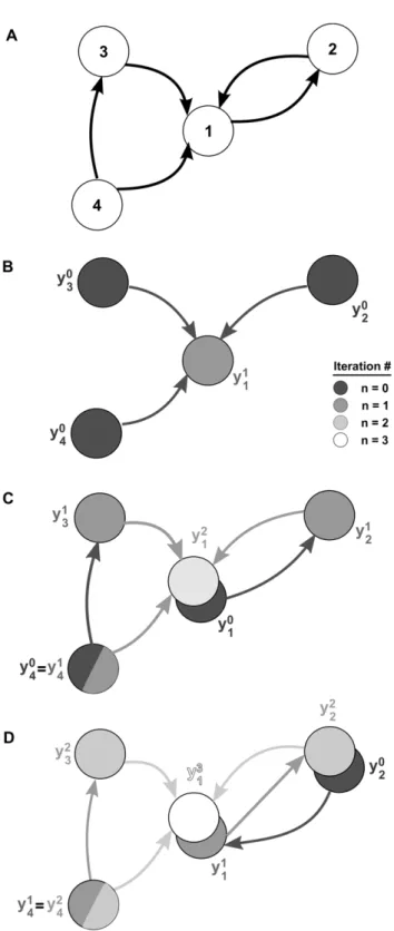
We therefore propose an iterative approach which accounts for successively larger connectivity patterns in the network [32,33]. We again start withy0i(t), a realization of a single spike train in isolation. Successive approximations to the output of cells in a recurrent network are defined by
ynz1 i (t)~y
0 i(t)z
X
j
(Kij ½ynj{rj)(t), n§0: ð10Þ
impact of next nearest neighbors. Successive iterations include the impact of directed chains of increasing length: The isolated output from an independent collection of neurons is filtered through n stages to produce the corrected response (See Figure 2.)
Notation is simplified when this iterative construction is recast in matrix form to obtain
ynz1(t) ~y0(t)z(K ½yn{r)(t) ~y0(t)znP
z1
k~1
(K(k) ½y0{r)(t), n§0, ð11Þ
whereyn(t)~½yn
i(t)andr~½riare lengthNcolumn vectors, and
K(k) represents a k-fold matrix convolution ofKwith itself. We define the convolution of matrices in the Methods.
The nth approximation to the matrix of cross-correlations can be written in terms of the interaction kernels, Kij, and the autocorrelations of the base processesy0as
Cij(t)&Cn(t) ~E(yn(tzt){r)(yn(t){r)T
~ P
n
k,l~0
(K(k)C0(K{
)(lT))(t), n§0, ð12Þ
where K{
(t)~K({t), X(kT)~(X(k))T, and X(k) is the k-fold matrix convolution ofXwith itself.
Eq. (12) can be verified by a simple calculation. First, Eq. (11) directly implies that
yn(t)~y0(t)zX n
k~1
(Kk ½y0{r)(t), n§0,
which we may use to find, for eachn§0,
Cn(t) :E(yn(tzt){r)(yn(t){r)T ~E(y0(tzt){r)(y0(t){r)T
zP
n
k~1
E(Kk ½y0{r)(tzt)(y0(t){r)T
z P
n
k~1
E(y0(tzt){r)(Kk ½y0{r)T(t)
z P
n
k,l~1
E(Kk ½y0{r)(tzt)(Kl ½y0{r)T(t)
~C0(t)zP n
k~1
(KkC0)(t)z P n
k~1
(C0(K{
)kT)(t)
z P
n
k,l~1
(KkC0(K{
)lT)(t):
ð13Þ
SinceK0ij(t)~dijd(t), Eq. (13) is equivalent to Eq. (12).
If we apply the Fourier transform, to Eq. (12), we find that for eachv,
Figure 2. Iterative construction of the linear approximation to
network activity. (A) An example recurrent network. (B)–(D) A
sequence of graphs determines the successive approximations to the output of neuron 1. Processes defined by the same iteration of Eq. (11) have equal color. (B) In the first iteration of Eq. (11), the output of neuron 1 is approximated using the unperturbed outputs of its neighbors. (C) In the second iteration the results of the first iteration are used to define the inputs to the neuron. For instance, the processy1 2
depends on the base process y0
1 which represents the unperturbed
output of neuron 1. Neuron 4 receives no inputs from the rest of the network, and all approximations involve only its unperturbed output,
y0
4. (D) Cells 3 and 4 are not part of recurrent paths, and their
contributions to the approximation are fixed after the second iteration. However, the recurrent connection between cells 1 and 2 implies that subsequent approximations involve contributions of directed chains of increasing length.
~
Cn(v)~E½~yn(v)~yn(v) ~ P n
k,l~0
~
Kk(v)E½~y0(v)~y0(v)(K~)l(v)
~ X
n
k~0
~ Kk(v)
!
E ~y0(v)~y0(v)
Xn
l~0 (~K)l(v)
!
,
ð14Þ
where X denotes the conjugate transpose of the matrix X. As before, the zero-mean Fourier transforms~yyn
i of the processesyni are defined by~yyn
i~F ½yni{ri, and~ff~F(f)for all other quantities. DefiningY(X)to be the spectral radius of the matrixX, when Y(KK~)v1, we can take the limit n?? in Eq. (14) [47,48], to obtain an approximation to the full array of cross-spectra
~
C(v)&C~?(v)~lim n??
~ Cn(v)
~(I{K~(v)){1C~0(v)(I{K~(v)){1: ð 15Þ
As noted previously, this generalizes the approach of Lindner et al. [26] (also see [13]). In the limitn??, directed paths of arbitrary length contribute to the approximation. Equation (15) therefore takes into account the full recurrent structure of the network. Note that Eq. (15) may be valid even whenY(KK~)w1. However, in this case the series in Eq. (14) do not converge, and hence the expansion of the correlations in terms of paths through the network is invalid. We confirmed numerically thatY(KK~)v1for all of the networks and parameters we considered.
Finally, consider the network response to external signals,gi(t), with zero mean and finite variance. The response of the neurons in the recurrent network can be approximated iteratively by
ynz1~y0zK
½yn{rzAg,
where A~diag(Ai) and g(t)~½gi(t). External signals and recurrent synaptic inputs are both linearly filtered to approximate a cell’s response, consistent with a generalization of Eq. (4). As in Eq. (12), thenthapproximation to the matrix of correlations is
C(t)&Cn(t)~ X n
k,l~0
(K(k)C0(K{
)(lT))(t)z
X n{1
k,l~0
(K(k)ACg(A{
)(K{
)(lT))(t),
where Ch(t)~Eg(tzt)g(t)T is the covariance matrix of the
external signals. We can again take the Fourier transform and the limitn??, and solve forCC~(v). IfY(KK~)v1,
~
C
C?(v)~(I{KK~(v)){1(CC~0(v)zAA~(v)CC~g(v)AA~(v))(I{KK~(v)){1:
ð16Þ
When the signals comprisinggare white (and possibly correlated)
corrections must be made to account for the change in spectrum and response properties of the isolated cells [26,49,50] (See Methods).
We note that Eq. (11), which is the basis of our iterative approach, provides an approximation to the network’s output which is of higher than first order in connection strength. This may seem at odds with a theory that provides a linear correction to a cell’s
response,cf.Eq. (4). However, Eq. (11) does not capture nonlinear corrections to the response of individual cells, as the output of each cell is determined linearly from its input. It is the input that can contain terms of any order in connection strength stemming from directed paths of different lengths through the network.
We use the theoretical framework developed above to analyze the statistical structure of the spiking activity in a network of IF neurons described by Eq. (1). We first show that the cross-correlation functions between cells in two small networks can be studied in terms of contributions from directed paths through the network. We use a similar approach to understand the structure of correlations in larger all–to–all and random networks. We show that in networks where inhibition and excitation are tuned to exactly balance, only local interactions contribute to correlations. When such balance is broken by a relative elevation of inhibition, the result may be increased synchrony in the network. The theory also allows us to obtain averages of cross-correlation functions conditioned on connectivity between pairs of cells in random networks. Such averages can provide a tractable yet accurate description of the joint statistics of spiking in these networks.
The correlation structure is determined by the response properties of cells together with synaptic dynamics and network architecture. Network interactions are described by the matrix of synaptic filters,
J, given in Eq. (2), while the response of cell i to an input is approximated using its linear response kernelAi. Synaptic dynamics, architecture, and cell responses are all combined in the matrixK, whereKijdescribes the response of cellito an input from cellj(See Eq. (1)). The correlation structure of network activity is approxi-mated in Eq. (15) using the Fourier transforms of the interaction matrix,K, and the matrix of unperturbed autocorrelationsC0. Statistics of the response of microcircuits
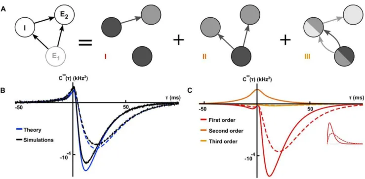
We first consider a pair of simple microcircuits to highlight some of the features of the theory. We start with the three cell model of feed-forward inhibition (FFI) shown in Figure 3A [51]. The interaction matrix,KK~(v), has the form
~
K K(v)~
0 0 0
~ K
KE2E1(v) 0 KKE~ 2I(v) ~
K
KIE1(v) 0 0 0 B @ 1 C A,
where cells are indexed in the orderE1,E2,I. To simplify notation, we omit the dependence ofKK~(v)and other spectral quantities on v.
Note that KK~ is nilpotent of degree 3 (that is,KK~3:0), and the inverse of(I{KK~)may be expressed as
(I{KK~){1~(
IzKK~zKK~2)~
1 0 0
~ K
KE2E1zKK~E2IKK~IE1 1 KK~E2I ~
K
KIE1 0 1
0
B @
1
C A:ð17Þ
Substituting Eq. (17) into Eq. (15) (and noting that a similar equation as Eq. (17) holds for(I{KK~){1) yields an approximation to the matrix of cross-spectra. For instance,
~ C C?
E2I~KKE~ 2ICC~ 0
IzKKE~ 2E1KK~
IE1CC~0E1zKEK~ 2IDKKIE~ 1D 2CC~0
E1
~(AAE~ 2~JJE 2I)CC~
0 I |fflfflfflfflfflfflfflfflffl{zfflfflfflfflfflfflfflfflffl}
I
z(AAE~ 2JJE~
2E1)(AAI~ JJIE~ 1)CC~ 0 E1 |fflfflfflfflfflfflfflfflfflfflfflfflfflfflfflfflfflfflfflfflffl{zfflfflfflfflfflfflfflfflfflfflfflfflfflfflfflfflfflfflfflfflffl}
II
z(AAE~ 2JJE~
2E1)DAAI~ ~JJIE1D 2CC~0
E1 |fflfflfflfflfflfflfflfflfflfflfflfflfflfflfflfflfflfflfflffl{zfflfflfflfflfflfflfflfflfflfflfflfflfflfflfflfflfflfflfflffl}
III
:
Figure 3B shows that these approximations closely match numerically obtained cross-correlations. CC~0
X is the uncoupled power spectrum for cellX.
Equation (18) gives insight into how the joint response of cells in this circuit is shaped by the features of the network. The three terms in Eq. (18) are directly related to the architecture of the microcircuit: Term I represents the correlating effect of the direct input to cellE2 from cellI. Term II captures the effect of the common input from cell E1. Finally, term III represents the interaction of the indirect input fromE1toE2throughIwith the input from E1 to I (See Figure 3C). A change in any single parameter may affect multiple terms. However, the individual contributions of all three terms are apparent.
To illustrate the impact of synaptic properties on the cross-correlation between cellsE2andI we varied the inhibitory time constant,tI (See Figure 3B and C). Such a change is primarily reflected in the shape of the first order term, I: Multiplication by ~
J
JE2Iis equivalent to convolution with the inhibitory synaptic filter, JE2I. The shape of this filter is determined bytI(See Eq. (2)), and a shorter time constant leads to a tighter timing dependency between the spikes of the two cells [24,52–55]. In particular, Ostojic et al. made similar observations using a related approximation. In the FFI circuit, the first and second order terms, I and II, are dominant (red and dark orange, Figure 3B). The relative magnitude of the third order term, III (light orange, Figure 3B), is small. The next example shows that even in a simple recurrent circuit, terms of order higher than two may be significant.
More generally, the interaction matrices, KK~, of recurrent networks are not nilpotent. Consider two reciprocally coupled excitatory cells,E1andE2(See Figure 4A, left). In this case,
~
K K~
0 KKE~ 1E2 ~
K
KE2E1 0 !
so that
(I{KK~){1~ 1 1{KKE~ 1E2KKE~ 2E1
(IzKK~):
Equation (15) gives the following approximation to the matrix of cross-spectra
~
C? ~ 1 j1{KKE~ 1E2KKE~ 2E1j2
(IzK~) ~ C C0
E1 0
0 CC~0 E2 0
@
1
A(IzK~)
~ 1
j1{KKE~ 1E2KKE~ 2E1j2 ~
C C0
E1zjKKE~ 1E2j 2~
C C0
E2 KK~E2E1CC~E01zKKE~ 1E2CC~ 0 E2
KE2E1CC~0E1zKE1E2CC~E02 CC~E02zjKE2E1j 2CC~0
E1 0
@
1
A:
ð19Þ
In contrast to the previous example, this approximation does not terminate at finite order in interaction strength. After expanding, the cross-spectrum between cells E1 and E2 is approximated by
Figure 3. The relation between correlation structure and response statistics in a feed-forward inhibitory microcircuit.(A) The FFI
circuit (left) can be decomposed into three submotifs. Equation (18) shows that each submotif provides a specific contribution to the cross-correlation between cellsE2andI. (B) Comparison of the theoretical prediction with the numerically computed cross-correlation between cellsE2
and I. Results are shown for two different values of the inhibitory time constant,tI (tI~5ms, solid line, tI~10ms, dashed line). (C) The contributions of the different submotifs in panel A are shown for bothtI~5ms (solid) andtI~10ms (dashed). Inset shows the corresponding
change in the inhibitory synaptic filter. The present color scheme is used in subsequent figures. Connection strengths were +40 mV:msfor excitatory and inhibitory connections. In each case, the long window correlation coefficientr(?)between the two cells was&{0:18.
~ C C?
E1E2~ X?
k,l~0 (KKE~
1E2KKE~ 2E1) k(KK~
E1E2KK~E2E1) l
(KK~E 2E1
~ C C0E
1z ~ K
KE1E2CC~E02):
ð20Þ
Directed paths beginning atE1and ending atE2(or vice-versa) are of odd length. Hence, this approximation contains only odd powers of the kernels KK~EiEj, each corresponding to a directed path from one cell to the other. Likewise, the approximate power spectra contain only even powers of the kernels corresponding to directed paths that connect a cell to itself (See Figure 4A).
The contributions of different sub-motifs to the cross- and auto-correlations are shown in Figures 4C, D when the isolated cells are in a near-threshold excitable state (CV&0:98). The auto-correlations are significantly affected by network interactions. We also note that chains of length two and three (the second and third submotifs in Figure 4A) provide significant contributions. Earlier approximations do not capture such corrections [24].
The operating point of a cell is set by its parameters (ti,EL,i, etc.) and the statistics of its input (Ei,si). A change in operating point can significantly change a cell’s response to an input. Using linear response theory, these changes are reflected in the response functionsAi, and the power spectra of the isolated cells,CC~0. To highlight the role that the operating point plays in the approximation of the correlation structure given by Eq. (15), we
Figure 4. The relation between correlation structure and response statistics for two bidirectionally coupled, excitatory cells.(A) The
cross-correlation between the two cells can be represented in terms of contributions from an infinite sequence of submotifs (See Eq. (20)). Though we show only a few ‘‘chain’’ motifs in one direction, one should note that there will also be contributions to the cross-correlation from chain motifs in the reverse direction in addition to indirect common input motifs (See the discussion of Figure 5). (B), (E) Linear response kernels in the excitable (B) and oscillatory (E) regimes. (C), (F) The cross-correlation function computed from simulations and theoretical predictions with first and third order contributions computed using Eq. (19) in the excitable (C) and oscillatory (F) regimes. (D), (G) The auto-correlation function computed from simulations and theoretical predictions with zeroth and second order contributions computed using Eq. (19) in the excitable (D) and oscillatory (G) regimes. In the oscillatory regime, higher order contributions were small relative to first order contributions and are therefore not shown. The network’s symmetry implies that cross-correlations are symmetric, and we only show them for positive times. Connection strengths were40 mV:ms. The long window correlation coefficientr(?)between the two cells was&0:8in the excitable regime and&0:5in the oscillatory regime. The ISI CV was approximately 0.98 for neurons in the excitable regime and 0.31 for neurons in the oscillatory regime.
elevated the mean and decreased the variance of background noise by increasing Ei and decreasingsi in Eq. (1). With the chosen parameters the isolated cells are in a super-threshold, low noise regime and fire nearly periodically (CV&0:31). After the cells are coupled, this oscillatory behavior is reflected in the cross- and auto-correlations where the dominant contributions are due to first and zeroth order terms, respectively (See Figures 4F,G).
Orders of coupling interactions. It is often useful to expand Eq. (15) in terms of powers of KK~ [31]. The term
~
K
KnCC~0(KK~)m in the expansion is said to be of order nzm. Equivalently, in the expansion ofCC~?ij, the order of a term refers to the sum of the powers of all constituent interaction kernelsKK~ab. We can also associate a particular connectivity submotif with each term. In particular,nth order terms of the form
~
K
Kian{1KK~an{1an{2 KK~a 1jCC~
0 jj
are associated with a directed pathj?a1? ?an{2?an{1?i from celljto celli. Similarly, the termCC~0iiKK~ia
1 KK~
an{2an{1KK~ an{1j corresponds to an-step path from cellito cellj. An(nzm)thorder term of the form
~
K
Kian{1KK~an{1an{2 KK~a 1a0CC~
0
a0a0KK~a0b1 KK~bm{2bm{1KK~ bm{1j
represents the effects of an indirect common inputnsteps removed from celliandmsteps removed from cellj. This corresponds to a submotif of the form i/an{1/ /a0?b1? ?bn{1?j consisting of two branches originating at cell a0. (See Figure 5, and also Figure 6A and the discussion around Eqs. (18,20).)
Statistics of the response of large networks
The full power of the present approach becomes evident when analyzing the activity of larger networks. We again illustrate the theory using several examples. In networks where inhibition and excitation are tuned to be precisely balanced, the theory shows
that only local interactions contribute to correlations. When this balance is broken, terms corresponding to longer paths through the network shape the cross-correlation functions. One conse-quence is that a relative increase in inhibition can lead to elevated network synchrony. We also show how to obtain tractable and accurate approximation of the average correlation structure in random networks.
A symmetric, all–to–all network of excitatory and inhibitory neurons. We begin with an all–to–all coupled network ofN identical cells. Of these cells,NE make excitatory, andNImake inhibitory synaptic connections. The excitatory cells are assigned indices 1,. . .,NE, and the inhibitory cells indices NEz1,. . .,N. All excitatory (inhibitory) synapses have weight WE~GE
NE (WI~ GI
NI), and timescale tE (tI). The interaction matrixKK~ may then be written in block form,
~
K
K~AA~JJ~, where JJ~~ ~ J
JE1NE NE JJI~1NE NI
~ J
JE1NI NE ~JJI1NI NI
!
:
Here 1N1N2 is the N1|N2 matrix of ones, ~JJX is the weighted synaptic kernel for cells of classX(assumed identical within each class), and AA~ is the susceptibility function for each cell in the network. Although the effect of autaptic connections (those from a cell to itself) is negligible (See Figure S2 in Text S1), their inclusion significantly simplifies the resulting expressions.
We define m~mE~NE~JJE,~mmI~NIJI~J, and mm~~mm~Ez~mmI. Using induction, we can show that
~
K
Kk~AA~kmm~k{1~JJ: Direct matrix multiplication yields
~
J
J~JJ~mm~c1NN where mm~c~NED~JJED2zNIDJJI~D2,
Figure 5. The motifs giving rise to terms in the expansion of Eq. (15).(A) Terms containing only unconjugated (or only conjugated)
interaction kernelsKK~
abcorrespond to directed chains. (B) Terms containing both unconjugated and conjugated interaction kernelsKK~abcorrespond to
which allows us to calculate the powersKK~kKK~lwhenk,l=0,
~
K
KkKK~l~AA~k(AA~)l~mmk{1( ~ m m)l{1
~ m mc1NN:
An application of Eq. (15) then gives an approximation to the matrix of cross-spectra:
~
C?~CC~0 X
?
k,l~0
~ KkK~l~
~ C C0 AA~
1{AA~~mm !
~ Jz
~ A A 1{AA~~mm
!
~ Jz
~ A A 1{AA~~mm
2
~ m
mc1NNzIN
" # ð21Þ
The cross-spectrum between two cells in the network is therefore given by
½C~?iji[X,j[Y~
~ C
C0 AA~ 1{AA~~mm
! ~ m mY NYz
~ A A 1{AA~~mm
! ~ m mX NXz
~ A A 1{AA~~mm
2
~ m mczdij
" #
, ð 22Þ
whereX,Y[fE,Ig. In Eq. (22) the first two terms represent the effects of all unidirectional chains originating at cell j and terminating at cell i, and vice versa. To see this, one should expand the denominators as power series inAA~~mm. The third term represents the effects of direct and indirect common inputs to the two neurons, which can be seen by expanding this denominator as a product of power series in AA~~mm and (AA~~mm). In Figure 6A, we highlight a few of these contributing motifs.
Interestingly, when excitation and inhibition are tuned for precise balance (so that the mean excitatory and inhibitory synaptic currents cancel, and~mm~~mmEzmm~I~0). Using~mm~0in Eq. (22) yields
½CC~?
i[X,j[Y~CC~0 AA~ ~ m mY NYzAA~
~mmX NXzDAAD~
2mm~ czdij
: ð23Þ
Effects of direct connections between the cells are captured by the first two terms, while those of direct common inputs to the pair are captured by the third term. Contributions from other paths do not
appear at any order. In other words,in the precisely balanced case only local interactions contribute to correlations.
To understand this cancelation intuitively, consider the contribution of directed chains originating at a given excitatory neuron, j. For tw0, the cross-correlation function, Cij(t), is determined by the change in firing rate of celliat timetgiven a spike in cell j at time 0. By the symmetry of the all–to–all connectivity and stationarity, the firing of cell j has an equal probability of eliciting a spike in any excitatory or inhibitory cell in the network. Due to the precise synaptic balance, the postsynaptic current generated by the elicited spikes in the excitatory population will cancel the postsynaptic current due to elicited spikes in the inhibitory population on average. The contribution of other motifs cancel in a similar way.
In Figure 6B, we show the impact of breaking this excitatory-inhibitory balance on cross-correlation functions. We increased the strength and speed of the inhibitory synapses relative to excitatory synapses, while holding constant, for sake of compar-ison, the long window correlation coefficients r(?) between excitatory pairs (note that, by symmetry, all excitatory pairs should have the same correlation coefficient). Moreover, the degree of network synchrony, characterized by the short window correlation coefficients, is increased (See Figure 6B inset). Intuitively, a spike in one of the excitatory cells transiently increases the likelihood of spiking in all other cells in the network. Since inhibition in the network is stronger and faster than excitation, these additional spikes will transiently decrease the likelihood of spiking in twice removed cells.
Linear response theory allows us to confirm this heuristic observation, and quantify the impact of the imbalance on second order statistics. Expanding Eq. (22) for two excitatory cells to second order in coupling strength, we find
~ C
C?EiEj~CC~0AA~mm~E NEzAA~
~mmE NEzjAA~j
2 ~ m
mczAA~2~mm~mmE NEz(AA~
)2~mmmm~E NEzdij
zO(jjK~jj3):
ð24Þ
Compared to the balanced case, there is no longer a complete cancellation between contributions of chains involving excitatory and inhibitory cells, and the two underlined terms appear as a result (compare with Eq. (23)). These terms capture the effects of
Figure 6. All–to–all networks and the importance of higher order motifs.(A) Some of the submotifs contributing to correlations in the all–
to–all network. (B) Cross-correlations between two excitatory cells in an all–to-all network (NE~80,NI~20) obtained using Eq. (21) (Solid – precisely tuned network with~mm:0[GE~{GI~140mVms,tE~tI~10ms], dashed – non-precisely tuned network withmm~=0[GE~168mVms,GI~{210mVms,
tE~10ms,tI~5ms]). (C) Comparison of first and second order contributions to the cross-correlation function in panel A in the precisely tuned (left) and
all length two chains between cellsEiorEj, starting at one and terminating at the other. The relative strengthening of inhibition implies that chains of length two provide a negative contribution to the cross-correlation function at short times (cf. [56], see the dashed orange lines in Figure 6C). Additionally, the impact of direct common input to cells Ei and Ej on correlations is both larger in magnitude (because we increased the strength of both connection types) and sharper (the faster inhibitory time constant means common inhibitory inputs induce sharper correlations). These changes are reflected in the shape of the second order, common input termDAAD~2mm~cin Eq. (24) (see dotted orange lines in Figure 6C).
In sum, unbalancing excitatory and inhibitory connections via stronger, faster inhibitory synapses enhances synchrony, moving a greater proportion of the covariance mass closer to t~0 (See Figure 6B). To illustrate this effect in terms of underlying connectivity motifs, we show the contributions of length two chains and common input in both the precisely tuned and non-precisely tuned cases in Figure 6C. A similar approach would allow us to understand the impact of a wide range of changes in cellular or synaptic dynamics on the structure of correlations across networks.
Random, fixed in-degree networks of homogeneous excitatory and inhibitory neurons. Connectivity in cortical
neuronal networks is typically sparse, and connection probabilities can follow distinct rules depending on area and layer [57]. The present theory allows us to consider arbitrary architectures, as we now illustrate.
We consider a randomly connected network ofNEexcitatory and NI inhibitory cells coupled with probability p. To simplify the analysis, every cell receives exactly pNE excitatory and pNI inhibitory inputs. Thus, having fixed in-degree (that is, the number of inputs is fixed and constant across cells), each cell receives an identical level of mean synaptic input. In addition, we continue to assume that cells are identical. Therefore, the response of each cell in the network is described by the same linear response kernel. The excitatory and inhibitory connection strengths areGE=(pNE)and GI=(pNI), respectively. The timescales of excitation and inhibition may differ, but are again identical for cells within each class.
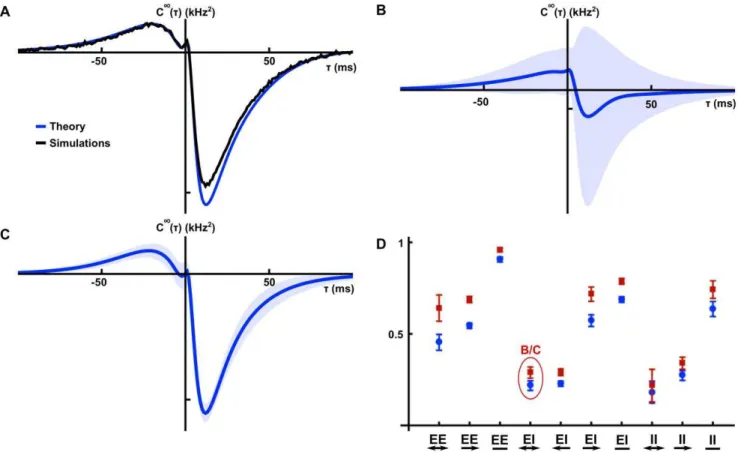
The approximation of network correlations (Eq. (15)) depends on the realization of the connectivity matrix. For a fixed realization, the underlying equations can be solved numerically to approximate the correlation structure (See Figure 7A). How-ever, the cross-correlation between a pair of cells of given types has a form which is easy to analyze when only leading order terms in 1=N are retained.
Specifically, the average cross-spectrum for two cells of given types is (See Section 1 in Text S1)
Figure 7. Correlations in random, fixed in-degree networks.(A) A comparison of numerically obtained excitatory-inhibitory cross-correlations
to the approximation given by Eq. (26). (B) Mean and standard deviation for the distribution of correlation functions for excitatory-inhibitory pairs of cells. (Solid line – mean cross-correlation, shaded area – one standard deviation from the mean, calculated using bootstrapping in a single network realization). (C) Mean and standard deviation for the distribution of cross-correlation functions conditioned on cell typeandfirst order connectivity for a reciprocally coupled excitatory-inhibitory pair of cells. (Solid line – mean cross-correlation function, shaded area – one standard deviation from the mean found by bootstrapping). (D) Average reduction inL2error between cross-correlation functions and their respective first-order conditioned
averages, relative to the error between the cross-correlations and their cell-type averages. Blue circles give results for a precisely tuned network, and red squares for a network with stronger, faster inhibition. Error bars indicate two standard errors above and below the mean.GE,GI,tE,tIfor panels A-C are as in the precisely tuned network of Figure 6, and the two networks of panel D are as in the networks of the same figure.
EnC~?ijo
i[X,j[Y
~CC~0 AA~ 1{AA~~mm
! " ~ m mY NYz ~ A A 1{AA~~mm
! ~ m mX NXz
~ A A 1{AA~~mm 2 ~ m mc 3
5zO1=N2,
ð25Þ
when i=j. This shows that, to leading order in 1=N, the mean cross-spectrum between two cells in given classes equals that in the all–to–all network (see Eq. (22)). Therefore our previous discussion relating network architecture to the shape of cross-correlations in the all–to–all network extends to the average correlation structure in the random network for largeN.
Pernice et al. [31] derived similar expressions for the correlation functions in networks of interactingHawkes processes[58,59], which are linear, self-exciting point processes with history-dependent intensities. They assumed that either the network is regular (i.e., both in- and out-degrees are fixed) or has a sufficiently narrow degree distribution. Our analysis depends on having fixed in-degrees, and we do not assume that networks are fully regular. Both approaches lead to results that hold approximately (for large enoughN) when the in-degree is not fixed.
Average correlations between cells in the random network conditioned on first order connectivity. As Figure 7B shows there is large variability around the mean excitatory-inhibitory cross-correlation function given by the leading order term of Eq. (25). Therefore, understanding the average cross-correlation between cells of given types does not necessarily provide much insight into the mechanisms that shape correlations on the level of individual cell pairs. Instead, we examine the average correlation between a pair of cells conditioned on their first order (direct) connectivity.
We derive expressions for first order conditional averages correct toO(1=N2)(See Section 2 in Text S1). The average cross-spectrum for a pair of cells with indicesi=j, conditioned on the value of the direct connections between them is
E C~?ijjJ~ij,J~ji
n o
i[X,j[Y ~
~ C
C0AA~J~ijzAA~J~jiz ~ A A2~mm 1{AA~~mm
! ~ m mY NYz ~ A A2mm~ 1{AA~~mm
! ~ m m X NXz ~ A A 1{AA~~mm 2 ~ m mc " #
zO(1=N2):
ð26Þ
Here we setJJ~ij~0if we condition on the absence of a connection j?i, and~JJij~JY=pJ~ if we condition on its presence. The termJJ~jiis set similarly.
Although Eq. (26) appears significantly more complicated than the cell-type averages given in Eq. (25), they only differ in the underlined, first order terms. The magnitude of expected contributions from all higher order motifs is unchanged and coincides with those in the all–to–all network.
Figure 7C shows the mean cross-correlation function for mutually coupled excitatory-inhibitory pairs. Taking into account the mutual coupling significantly reduces variability (Compare with Figure 7B). To quantify this reduction, we calculate the mean reduction in variability when correlation functions are computed conditioned on the connectivity between the cells. For a single network, the relative decrease in variability can be quantified using
merror~ 1 NT
X
(i,j)[T iwj
DDCij(t){CTFOC(t)DD2 DDCij(t){CCTT (t)DD2
,
whereTrepresents pairs of cells of a given type and connection (in the present example these are reciprocally coupled excitatory-inhibitory pairs), NT is the number of pairs of that type in the network, CCT
T (t) is the leading order approximation of average correlations given only the type of cells inT (as in Eq. (25)), and CFOC
T (t)the leading order approximation to average correlations conditioned on the first order connectivity of classT (as in Eq. (26)). We make use of the normDD:DD2defined byDDfDD2~ ÐDfD21=2. Figure 7D shows merror averaged over twenty networks. In particular, compare the reduction in variability when conditioning on bidirectional coupling between excitatory-inhibitory pairs shown in Figures 7B,C, with the corresponding relative error in Figure 7D (circled in red).
Discussion
We have extended and further developed a general theoretical framework that can be used to describe the correlation structure in a network of spiking cells. The application of linear response theory allows us to find tractable approximations of cross-correlation functions in terms of the network architecture and single cell response properties. The approach was originally used to derive analytical approximations to auto- and cross-spectra in an all–to–all inhibitory network in order to study the population response of the electrosensory lateral line lobe of weakly electric fish [26]. The key approximation relies on the assumption that the activity of cells in the network can be represented by a mixed point and continuous stochastic process, as given in Eq. (9). This approximation may be viewed as a generalization of classic Linear-Poisson models of neural spiking: the crucial difference is the replacement of the stationary firing rate by a realization of an integrate-and-fire spiking process. This allows for the retention of the underlying IF spiking activity while additionally posing that neurons act as perfect linear filters of their inputs. An iterative construction then leads to the expressions for approximate cross-correlations between pairs of cells given by Eq. (15).
The linear response framework of Lindner et al. [26] was extended by Marinazzo et al. [60] to somewhat more complex networks, and compared with other studies in which networks exhibit collective oscillations. In addition, other works [13,61,62] used linear response techniques to study information in the collective response of cells in a network. More recently, Ostojic et al. [24] obtained formulas for cross-correlations given in Eq. (9), which correspond to the first step in the iterative construction. Their approach captures corrections due to direct coupling (first order terms) and direct common input (second order terms involving second powers of interaction kernels; see also [49,63]). Our approach can be viewed as a generalization that also accounts for length two directed chains, along with all higher order corrections. As Figure 4 illustrates, these additional terms can be significant. The present approach also allows us to calculate corrected auto-correlations, in contrast with that of Ostojic et al.
Our work is also closely related to that of Pernice et al. [31], who analyzed the correlation structure in networks of interacting
functions. However, as they note, their approach can be extended to obtain the temporal structure of cross-correlations. Similarly, Toyoizumi et al. [64] derive expressions for cross-correlations in networks of interacting point process models in the Generalized Linear Model (GLM) class. These are very similar to Hawkes processes, but feature a static nonlinearity that shapes the spike emission rate.
To illustrate the power of the present linear response theory in analyzing the factors that shape correlations, we considered a number of simple examples for which the approximation given by Eq. (15) is tractable. We showed how the theory can be used both to gain intuition about the network and cell properties that shape correlations, and to quantify their impact. In particular, we explained how only local connections affect correlations in a precisely tuned all–to–all network, and how strengthening inhibition may synchronize spiking activity. In each case, we use comparisons with integrate-and-fire simulations to show that linear response theory makes highly accurate predictions.
It may be surprising thatlinearresponse theory can be used to provide corrections to cross-correlations of arbitrary order in network connectivity. The key to why this works lies in the accuracy of the linearization. A more accurate approximation could be obtained by including second and higher order corrections to the approximate response of a single cell, as well as corrections to the joint response. While including such terms is formally necessary to capture all contributions of a given order in network connectivity [32,33], the success of of linear response theory suggests that they are small for the cases at hand. In short, the present approximation neglects higher-order corrections to the approximate response of individual cells, along with all corrections involving joint responses, but accounts for paths through the network of arbitrary length.
As expected from the preceding discussion, simulations suggest that, for IF neurons, our approximations become less accurate as cells receive progressively stronger inputs. The physical reasons for this loss of accuracy could be related to interactions between the ‘‘hard threshold’’ and incoming synaptic inputs with short timescales. Additionally, while the theory will work for short synaptic timescales, it will improve for slower synaptic dynamics, limiting towards being essentially exact in the limit of arbitrarily long synaptic time constants (note the improvement in the approximation for the FFI circuit for the slower timescale exhibited in Figure 3). Another important factor is background noise, which is known to improve the accuracy of the linear description of single cell responses. We assume the presence of a white noise background, although it is possible to extend the present methods to colored background noise [25,65].
We found that linear response theory remains applicable in a wide range of dynamical regimes, including relatively low noise, superthreshold regimes where cells exhibit strong oscillatory behavior. Moreover, the theory can yield accurate approximations of strong correlations due to coupling: for the bidirectionally coupled excitatory circuit of Figure 4, the approximate cross-correlations match numerically obtained results even when correlation coefficients are large (rE1E2(?)&0:8in the excitable regime, &0:5in the oscillatory regime). Additional discussion of the limits of applicability of linear response to the computation of correlations in networks can be found in the Supplementary Information. There, we show that the approximation is valid over a range of physiological values in the case of the all-to-all network, and that the theory gives accurate predictions in the presence of low firing rates (see Figures S3, S4 in Text S1).
The limits of linear response approximations of time-dependent firing activity and correlations have been tested in a number of
other studies. Ostojic and Brunel [66] examined this accuracy in the relatively simple case of a neuron receiving filtered Gaussian noise in addition to a white background. Chacron et al. [61] noted that linear response approaches applied to networks of perfect integrators begin to display significant errors at larger connection strengths. Marinazzo et al. [60] remarked on the errors induced by network effects in linear response approximations to correlations in a delayed feedback loop. In particular, these errors were attributed to network effects such as synchrony in the excitatory population. The authors noted that such activity can not be correctly modeled by a linear approach.
Although we have demonstrated the theory using networks of integrate–and–fire neurons, the approach is widely applicable. The linear response kernel and power spectrum for a general integrate and fire neuron model can be easily obtained [29]. In addition, it is also possible to obtain the rate, spectrum, and susceptibility for modulation of the mean conductance in the case of conductance-based (rather than current-based) synapses (See [67] and Section 3 in Text S1). As the linear response kernel is directly related to the spike triggered average [24,30], the proposed theoretical framework should be applicable even to actual neurons whose responses are characterized experimentally. The possibilities for future applications are numerous. For example, one open question is how well the theory can predict correlations in the presence of adaptive currents [67]. In addition, the description of correlations in terms of architecture and response properties suggests the possibility of addressing the difficult inverse problem of inferring architectural properties from correlations [22–24,64]. Ostojic et al. applied linear response methods to the latter problem. It is our hope that the present approach will prove a valuable tool in moving the computational neuroscience community towards a more complete understanding of the origin and impact of correlated activity in neuronal populations.
Methods
Measures of spike time correlation
We quantify dependencies between the responses of cells in the network using the spike train auto- and cross-correlation functions [39]. For a pair of spike trains,yi(t),yj(t), the cross-correlation functionCij(t)is defined as
Cij(t)~cov yi(tzt),yj(t):
The auto-correlation function Cii(t) is the cross-correlation between a spike train and itself, andC(t)is the matrix of cross-correlation functions. Denoting by Nyi(t1,t2)~Ðt2
t1yi(s)ds the number of spikes over a time window ½t1,t2, the spike count correlation,rij(T), over windows of lengthtis defined as,
rij(T)~
covNyi(t,tzT),Nyj(t,tzT) ffiffiffiffiffiffiffiffiffiffiffiffiffiffiffiffiffiffiffiffiffiffiffiffiffiffiffiffiffiffiffiffiffiffiffiffiffiffiffiffiffiffiffiffiffiffiffiffiffiffiffiffiffiffiffiffiffiffiffiffiffiffiffiffiffiffiffiffiffiffi varNyi(t,tzT)varNyj(t,tzT)
r :
We assume stationarity of the spiking processes (that is, the network has reached a steady state) so thatrij(T)does not depend ont. We also use the total correlation coefficientrij(?)~limT??rij(T)to characterize dependencies between the processesyi and yj over arbitrarily long timescales.
covNyi(t,tzT),Nyj(t,tzT)~ ðT
{T
Cij(t)(T{DtD)dt:
We can interpret the cross-correlation as the conditional probability that cell ispikes at timetztgiven that cell jspiked at timet. The conditional firing rate,
Hij(t)~lim Dt?0
1
DtPr Nyi(tzt,tztzDt)w0DNyj(t,tzDt)w0
,
is the firing rate of celliconditioned on a spike in celljattunits of time in the past, andCij(t)~rj(Hij(t){ri):
Define the Fourier transform of a function f(t) as ~
ff(v)~F ½f(t)(v):Ð{??f(t)e{2pivtdt: We will often make use of the cross-spectrum between the output of cells i,j, given by
~
C
Cij(v)~E ~yyi(v)~yyj(v)
h i
, which is the Fourier transform of the cross-correlation function of cellsi,j. The power spectrumCC~ii(v)is the cross-spectrum between a cell and itself, and is the Fourier transform of the auto-correlation function.
Numerical methods. Simulations were run in C++, and the stochastic differential equations were integrated with a standard Euler method with a time-step of 0.01 ms. General parameter values were as follows: ti~20ms, EL,izEi~{54mV, si~
ffiffiffiffiffi 12
p
mV, vth~
20mV, vr~{54mV, tref~2ms, VT~{52:5mV, DT~1:4mV, tE~10ms, tI~5ms, tD,i~1ms. Marginal statistics (firing rates, uncoupled power spectra and response functions) were obtained using the threshold integration method of [29] in MATLAB. We have posted a package of code which contains examples of all the numerical methods used in this paper (both simulations and theory) at http://www.math.uh.edu/,josic/myweb/software.html. Additional code is available upon request.
Calculation of stationary rates in a recurrent network. The stationary firing rate of an IF neuron can be computed as a function of the mean and intensity of internal noise (Ei,si) and other cellular parameters (ti,ELi, etc…) [69]. Denote
the stationary firing rate of cell iin the network by ri, and by ri,0(E,s) the stationary firing rate in the presence of white noise with meanEand variances2. We keep the dependencies on other parameters are implicit. The stationary rates,ri, in the recurrent network without external input are determined self-consistently by
ri~ri,0(Ei’,si)~ri,0(Eiz X
j
Wijrj,si) i~1,. . .,N,
where we used E½ fi~PjWijEyj~PjWijrj. This equality holds because the synaptic kernels,Jij, were normalized to have area Wij. These equations can typically be solved by fixed-point iteration.
Note that this provides an effective mean input,Ei’, to each cell,
but does not give adjustments to the variance,si. We assume that the major impact of recurrent input is reflected inEi’, and ignore
corrections to the cell response involving higher order statistics of the input. This approach is valid as long as fluctuations in the recurrent input to each cell are small compared tosi, and may break down otherwise [27].
Correction to statistics in the presence of an external white noise signals. Expression (16) can be used to compute
the statistics of the network response to inputs gi(t) of finite variance. As noted by [26], when inputs have infinite variance additional corrections are necessary. As a particular example, consider the case where the processes are correlated white noise, i.e., when gi(t)~pffiffifficxc(t)zpffiffiffiffiffiffiffiffiffiffi1{cxi(t), where xc,xi are independent white noise processes with variance se. Then each gi is also a white noise process with intensity se
i, but
Egi(tzt)gj(t)~½dijd(t)z(1{dij)cd(t)sei. The firing rate of celliin response to this input isri~r0(Ei’,
ffiffiffiffiffiffiffiffiffiffiffiffiffiffiffiffiffiffiffiffiffiffiffiffi (si)2z(sei)
2 q
), and the point around which the response of the cell is linearized needs to be adjusted.
Finally, we may apply an additional correction to the linear response approximation of autocorrelations. For simplicity, we ignore coupling in Eq. (16) (so thatKK~~0). Linear response predicts thatCC~ii(v)~CC~ii0(v;s2i)z(sei)
2DAAi~(v)D2
, where we have introduced explicit dependence on s2
i, the variance of white noise being received by an IF neuron with power spectrumCC~0ii(v;s2
i), in the absence of the external signal. The approximation may be improved in this case by making the following substitution in Eq. (16) [26,50]:
~
C
C0ii(v;s2i)z(sei)2DAAi~(v)D2 ? CC~0
ii(v;s2iz(sei)2)
The response functionAshould be adjusted likewise.
Convolution of matrices. Let X(t)~½Xij(t) and
Y(t)~½Yij(t) be n1|n2 and n2|n3 matrices of functions, respectively. We define the convolution of matrices(XY)(t) to be then1|n3matrix of functions with entries defined by
(XY)ij(t)~ X
k
(XikYkj)(t):
Expectations and convolutions commute for matrix convolutions as matrix expectations are taken entry-wise. Each entry of a matrix convolution is a linear combination of scalar convolutions which commute with expectations. Additionally, we adopt the convention that the zeroth power of the interaction matrix,
K0
ij(t), is the diagonal matrix withK0ij(t)~d(t)wheni~j. Hence
K0ij(t)acts as the identity matrix under matrix convolution. Supporting Information
Text S1 Supplementary information file containing derivations and additional content, such as an exploration of the error of the theory. Supporting information figures were included in this file (and not separately).
(PDF)
Acknowledgments
The authors thank Robert Rosenbaum, Brent Doiron and Srdjan Ostojic for many helpful discussions.
Author Contributions
Conceived and designed the experiments: JT YH ESB KJ. Performed the experiments: JT. Analyzed the data: JT. Contributed reagents/materials/ analysis tools: JT YH ESB KJ. Wrote the paper: JT YH ESB KJ.
References
1. Cohen M, Kohn A (2011) Measuring and interpreting neuronal correlations. Nat Neurosci 14: 811–819.