Dynamic decision making for dam-break emergency management – Part 1: Theoretical framework

www.nat-hazards-earth-syst-sci.net/13/425/2013/ doi:10.5194/nhess-13-425-2013

© Author(s) 2013. CC Attribution 3.0 License.

Natural Hazards

and Earth System

Sciences

Geoscientiic

Geoscientiic

Geoscientiic

Geoscientiic

Dynamic decision making for dam-break emergency management

– Part 1: Theoretical framework

M. Peng1,2and L. M. Zhang1

1_{Department of Civil and Environmental Engineering, The Hong Kong University of Science and Technology, Hong Kong} 2_{Key Laboratory of Geotechnical and Underground Engineering of Ministry of Education,}

Department of Geotechnical Engineering, Tongji University, Shanghai, China Correspondence to:L. M. Zhang (cezhangl@ust.hk)

Received: 26 March 2012 – Published in Nat. Hazards Earth Syst. Sci. Discuss.: –

Revised: 10 December 2012 – Accepted: 15 December 2012 – Published: 18 February 2013

Abstract.An evacuation decision for dam breaks is a very serious issue. A late decision may lead to loss of lives and properties, but a very early evacuation will incur unneces-sary expenses. This paper presents a risk-based framework of dynamic decision making for dam-break emergency man-agement (DYDEM). The dam-break emergency manman-agement in both time scale and space scale is introduced first to de-fine the dynamic decision problem. The probability of dam failure is taken as a stochastic process and estimated using a time-series analysis method. The flood consequences are taken as functions of warning time and evaluated with a hu-man risk analysis model (HURAM) based on Bayesian net-works. A decision criterion is suggested to decide whether to evacuate the population at risk (PAR) or to delay the deci-sion. The optimum time for evacuating the PAR is obtained by minimizing the expected total loss, which integrates the time-related probabilities and flood consequences. When a delayed decision is chosen, the decision making can be up-dated with available new information. A specific dam-break case study is presented in a companion paper to illustrate the application of this framework to complex dam-breaching problems.

1 Introduction

Dam breaks can cause catastrophic consequences to human beings. Past dam failure disasters have shown that flood risks are directly related to the available warning time (the period from issuing evacuation warning to the arrival moment of a flood) for evacuation. Despite the benefits of saving human

life and properties, an evacuation decision should be treated as a very serious issue since it often incurs a large amount of economic expense at the same time (Frieser, 2004). Be-fore making an evacuation decision, two problems need to be considered. Is it necessary to evacuate the population at risk (PAR)? If yes, then when is the optimal time to evacuate the PAR? The answers to these problems raise the need for proper decision-making based on dynamic risk analysis that considers time effects.

Generally, there are two categories of methods of decision making for emergency management: deterministic methods and probabilistic methods. Deterministic methods are those based on deterministic analysis, experiences and judgment without explicit consideration of uncertainties. In determin-istic methods, some critical values (e.g. water level, period return flood) are often suggested as indices for evacuation decision-making (Nielsen et al., 1994; Frieser, 2004). Some guidelines also offer recommendations for decision-making based on judgments (Urbina and Wolshon, 2003; FEMA, 2004). Deterministic methods are simple to apply. However, they may not be reasonable as the uncertainties are not stud-ied.

Table 1.Flood consequences

Category Consequence Influenced by Influenced by Considered

evacuation? warning time? in DYDEM?

Evacuation cost

Initial evacuation cost Yes Increase Yes

GDP interruption by evacuation Yes Increase Yes

Indirect influence Yes Increase No

Flood damage

Immoveable properties No No influence No

Moveable properties Yes Decrease Yes

GDP interruption by flood No No influence No

Environmental damage No No influence No

Loss of life Fatalities Yes Decrease Yes

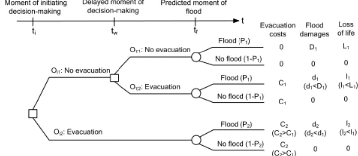
trees have been frequently used to conduct quantitatively risk-based decision making in mitigation of various disasters (Frieser, 2004; Smith et al., 2006; Lindell et al., 2007; Woo, 2008; Liu, 2009). Frieser (2004) and Smith et al. (2006) com-mented that the evacuation decision for floods can be delayed in cases with long prediction lead time and large uncertain-ties. Figure 1 shows a delayed decision tree for a flood dis-aster. The flood consequences include evacuation costs (C), flood damage (D), and loss of life (L) as shown in Table 1. Evacuation costs include initial costs (e.g. costs of transport, accommodation, food supply, organization and service), in-terruption of gross domestic product (GDP) due to evacua-tion, and indirect influences (e.g. influence of the market in the affected areas). The evacuation costs increase with the warning time. The indirect influences are difficult to evaluate and not included in this study. Flood damages include all the consequences caused by flooding except those to human life. Some moveable properties such as cars and portable items can be saved by evacuation. However, immoveable properties such as houses, GDP interruption and environmental dam-age cannot be reduced by evacuation. Therefore, those are not involved in this study. Loss of life is the fatality caused by flooding. Historical data show that the fatality rate can be largely reduced by allowing more warning time (DeKay and McClelland, 1993; Graham, 1999).

The evacuation may be delayed (e.g.twin Fig. 1) to obtain

information with less uncertainty and to reduce the evacu-ation costs (C1< C2), as shown in Fig. 1. As more

infor-mation is collected, the uncertainty in the dam failure prob-ability,P1, with a delayed decision is smaller than that in P2 in Fig. 1. However, such delayed evacuation runs the

risk of losing more lives (L1> l1> l2)and properties (D1> d1> d2)given less available time for evacuation. A good

de-cision should try to attain a minimum expected total loss. Time-dependent evacuation decision can be analyzed using a multi-phase decision tree (Frieser, 2004; Smith et al., 2006). The probabilistic methods using decision trees are superior to deterministic methods due to the inclusion of uncertainties.

A premise of using a decision tree in the existing meth-ods is to assume a predicted time of flooding,tf, as shown in

Flood (P1)

No flood (1-P1)

Evacuation costs

Flood damages 0 D1

0 C1

d1

(d1<D1) 0 Oi2: Evacuation

Oi1: No evacuation

Oτ2: Evacuation

Oτ1: No evacuation

C2

(C2>C1)

d2

(d2<d1)

0

ti tw tf

Delayed moment of decision-making Moment of initiating

decision-making

t

0

C2

(C2>C1)

C1

Loss of life L1

0 l1

(l1<L1) 0

l2

(l2<l1)

0 Predicted moment of

flood

Flood (P2)

No flood (1-P2)

Flood (P1)

No flood (1-P1)

Fig. 1.Decision tree for dam-break emergency management (mod-ified from Frieser, 2004).

Fig. 1. Normally,t_fis set as a target time (e.g. with enough lead time to evacuate the people) or the time of the worst predicted situation (e.g. the highest water level or largest flood flow rate). This may not be reasonable due to the fact that a dam-break flood may occur at any future time. There-fore, decision trees may not be sufficient for dynamic deci-sion making, since the predicted flood probability should be a stochastic process instead. The loss of life and properties could be underestimated if the flood occurs before the pre-dicted time, and vice versa.

Fig. 2.Schematic of the dam breaching and warning time.

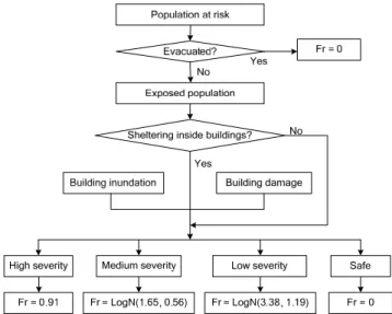
of this framework to complex dam-breaching problems. HU-RAM simulates the evacuation, sheltering and loss of life in a flood event, which are closely related to the evacuation cost, flood damage and number of fatalities in this paper. DYDEM in this paper focuses on dynamic decision making for dam-break emergency management.

2 Dam-break emergency management

Dam-break emergency management is aimed to minimize the possible dam-break consequences using primarily non-structural measures, such as warning, sheltering and evacu-ation. This section presents the dam-break emergency man-agement in both time and space scale to define the dynamic decision making problems.

2.1 In time scale

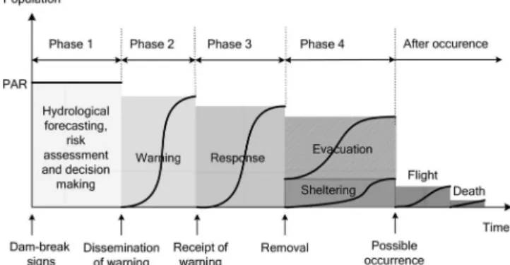
The prediction lead time (i.e. the duration between the pre-diction moment and the predicted failure time) of a dam-break flood is usually on the order of hours or days. Dur-ing this period emergency management can possibly be im-plemented to save human lives and properties. The studied time includes available time and demand time. The avail-able time is influenced by the dam breaching and flood rout-ing processes. The concepts of breachrout-ing and warnrout-ing time are shown in Fig. 2. The demand time for emergency man-agement can be divided into four phases: (1) hydrological forecasting, risk assessment and decision making; (2) warn-ing; (3) response; and (4) evacuation and sheltering (Frieser, 2004), as shown in Fig. 3.

Emergency management starts from the identification of signs of dam break (e.g. the water level rises to the crest or cracks in the dam) (Fig. 3). Risk assessment, based on the hydrological forecasting, must be conducted before the evac-uation decision making in phase 1. The government must de-cide the optimal time to evacuate the population at risk (PAR) if evacuation is finally chosen. It takes time to transmit warn-ing messages in phase 2. An S-curve for the PAR warned and the progress of warning is shown in Fig. 3. The warning transmitting time is defined as the duration between issuing the warning and the receipt of it. Phase 3 starts at the receipt

Fig. 3.Emergency management of dam breaks in time scale (modi-fied from Frieser, 2004).

of warning messages by the PAR. The PAR needs time to confirm the warning messages, prepare for evacuation and wait for family members. A part of the PAR may evacuate to safe places as shown in phase 4 of Fig. 3. The rest, ei-ther refusing to evacuate or having insufficient time, may try to shelter themselves in relatively safe places (e.g. high rise buildings) in the flooded areas. After the possible occurrence of the disaster, people may flee for safe havens. Some of these might lose their lives, however.

The dam-break emergency management in time scale dis-plays the sequence of human activities and the population distributions with time before the flood occurrence. A good decision should consider not only the available time before the predicted arrival of the flood, but also the demand time for each phase and the corresponding population distribution. 2.2 In space scale

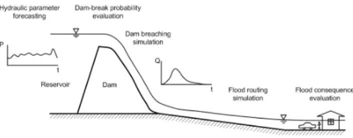
The risk analysis of a dam-break event covers a large area along the river from the catchment upstream of the dam to the potential flood areas downstream of the dam. In space scale (Fig. 4), the dam-break emergency management includes five steps: hydraulic parameter forecasting, dam-break probabil-ity evaluation, dam breaching simulation, flood routing sim-ulation and flood consequence evaluation.

Hydraulic parameters such as reservoir volume, inflow rate and water elevation directly influence the dam safety condi-tions. These parameters should be treated as stochastic pro-cesses instead of independent random variables due to the correlations in time scale.

Fig. 4.Emergency management of dam breaks in space scale.

reservoir water elevation exceeds the elevation of the dam crest. The probability of dam failure is closely related to hy-drological parameters.

The next two components are to simulate the dam breach-ing process and flood routbreach-ing downstream of the dam. The breaching parameters significantly affect the flood conse-quence downstream. In this study, an empirical model (Peng and Zhang, 2012c) based on statistical data is used to simu-late the breaching process when only geometrical parameters are available, while a physical model, DABA (Chang and Zhang, 2010), is used when more soil properties are avail-able (e.g. cohesion and friction angle). The outputs of the breaching simulation are peak outflow rate, breaching time and breach size. With the breaching parameters predicted, a river analysis program, HEC-RAS 4.0, developed by Hydro-logic Engineering Center (2008), is used to simulate the flood routing in the river downstream of the dam. Detailed simula-tions in a specific case will be introduced in the companion paper (Peng and Zhang, 2013).

The flood consequences, including evacuation costs, flood damage and loss of life as shown in Fig. 1, are highly related to the warning time. Generally, evacuation costs increase and flood damage and loss of life decrease with more warning time. The dam-break emergency management should cover the evolution of the dam-break event in space scale. A proper decision should take the dam-break probability as a time se-ries and the consequences as functions of warning time.

3 Framework of dynamic decision making

The framework of dynamic decision making is intended to make a decision whether to evacuate the population at risk or to delay the decision; to predict the optimal time to evacuate the PAR with the minimum expected total loss; and to update the decision-making with new information when delayed de-cision is chosen.

Assume a continuous stochastic process of dam-break probability as shown in Fig. 5. The studied period ranges fromt0 (e.g. the current time) to tend (e.g. the moment

af-ter which the risk is not considered). The probability of dam failure in a short period dtis calculated as

f(t)

t dt

Pre-warning After flood

Issuing evacuation

warning

Possible flood

Fig. 5.Probability of dam-break flood as a continuous stochastic process of time.

P (t )=f (t )dt (1)

wheref (t )is a continuous stochastic process of dam fail-ure probability. Given the time of issuing evacuation warn-ing (t0≤tw≤tend)as shown in Fig. 5, the period between t_w and possible flood arrival time (t_f)is called the warning time (Wt), which is critical for the people at risk to evacuate to safe places. Warning time equals zero if the possible flood occurs before the time for evacuating the PAR. Thus,Wt is a non-negative parameter and given by

Wt=0, whentf< tw (2)

Wt=tf−tw, whentf≥tw (3)

Wt=tend−tw,whentf≥tend. (4)

The flood risk, or expected total loss,E(Lt), is the sum of

the expected evacuation costs, flood damage and loss of life, which are obtained by integrating the product of these three categories of consequences and their corresponding proba-bilities along time:

E(Lt)=

Z

L(t )f (t )dt (5)

=

+∞ Z

t0

[C(Wt)+D(Wt)+L(Wt)]f (t )dt

=

+∞ Z

t0

C(Wt)f (t )dt+

+∞ Z

t0

[D(Wt)+L(Wt)]f (t )dt

whereL(t )is the flood consequences or total loss;C(Wt),

Fig. 6.Probability of dam-break flood as a discrete stochastic pro-cess of time.

+∞ Z

t0

C(Wt)f (t )dt= tw

Z

t0

C(0)f (t )dt

+

tend

Z

tw

C(t−tw)f (t )dt+C(tend−tw)[1−

tend

Z

t0

f (t )dt] (6)

+∞ Z

t0

[D(Wt)+L(Wt)]f (t )dt= tw

Z

0

[D(0)+L(0)]f (t )dt

+

tend

Z

tw

[D(t−tw)+L(t−tw)]f (t )dt+0. (7)

The last part of Eq. (6) denotes that evacuation costs incur even if there is no dam failure or if the failure time is beyond the studied period. The last part of Eq. (7) denotes that the flood damage and loss of life are not considered if there is no dam failure in the studied period.

The optimal time to evacuate the PAR is the time to attain the minimum total loss or the time at which the derivative of the following function is zero:

Min[E(Lt)]or

dE(Lt)

dt_w =0. (8)

For a discrete time series as shown in Fig. 6, the probabil-ity of flooding in the period fromtj−1totjis given byP (tj). The expected total loss is given by

E(Lt)=

+∞ X

j=1

L(tj)P (tj)

=

+∞ X

j=1

[C(Wt)+D(Wt)+L(Wt)]P (tj) (9)

Flood conse

quenc

es

Time of issuing evacuation warning

Total loss

Loss of life

Flood damage

Evacuation costs Optimal

point

Fig. 7.Flood consequences as functions of time for evacuating the PAR.

=

+∞ X

j=1

C(Wt)P (tj)

+

+∞ X

j=1

[D(Wt)+L(Wt)]P (tj). (10)

Similarly, considering the definition ofWtin Eqs. (2)–(4), Eq. (9) can be separated into two equations:

+∞ X

j=1

C(Wt)P (tj)= w

X

j=1

C(0)P (tj) (11)

+

N

X

j=w+1

C(tj−tw)P (tj)+C(tend−tw)[1−

N

X

j=0 P (tj)]

+∞ X

j=1

[D(Wt)+L(Wt)]P (tj)= w

X

j=1

[D(0)+L(0)]P (tj)

+

N

X

j=w+1

[D(tj−tw)+L(tj−tw)]P (tj)+0, (12)

where tN=tend. The optimal time to issue the

evacua-tion warning is the time to attain the minimum total loss [Min(E(Lt)].

Figure 7 shows the flood consequences as functions of the time for issuing warning (tw). The flood damage and loss

of life increase and the evacuation costs decrease withtw.

Therefore, there is an optimal point (top)for evacuating the

PAR to achieve the minimum expected total loss. The param-eter,t_op, is very important in decision making. Ift_op is close tot₀, the PAR should be evacuated immediately; ift_op=t_end, no evacuation is decided; ift0> top< tend, the PAR should

be evacuated attop. If it is not in an urgent case, namelytopis

much larger thant0, we may delay the decision to gain more

information to reduce the uncertainties.

As time goes on, more information for decision will be available. The decision with a different initial time (t0)is

evaluated results may be different. Thus, a dynamic deci-sion should be a multi-stage decideci-sion process, the details of which will be introduced in the companion paper (Peng and Zhang, 2013). In each stage, as the information gathered and its condition of uncertainty is different, the predicted dam-break probabilities and flood consequences could be differ-ent. It would be unnecessary to consider the decision making as a continuous process oft0since the changes in

informa-tion may be small in a short period. In this framework, the multi-stage decisions are limited to stages with significant changes in information, such as a predicted storm, changes in knowledge on the properties of the dam materials, and im-plementing major flood control measures. In the multi-stage decision framework, both the predicted dam-break probabil-ities and consequences should be updated in each new stage. This will be illustrated with a specific dam-break case study in the companion paper (Peng and Zhang, 2013).

It may be debatable to put a price on human life and make a decision with a minimal expected total loss. However, as the actual expenditures on risk reduction are finite, it may be rational to set a value of a life to help rational decision mak-ing. In this study, a value of the macroeconomic contribution of a person is used to monetize a human life, which will be introduced later. From the overview of the dynamic decision framework, two important components of the framework are critical: prediction of dam-break probability as a stochastic process and evaluation of flood consequences as functions of warning time. These two components will be presented in the next two sections.

4 Prediction of dam-break probability with time series 4.1 Dam-break probability analysis

As introduced above, only the overtopping failure mode is discussed in this paper. A dam is assumed to be overtopped once the reservoir volume exceeds its capacity (V_cr):

Vt> Vcr (13)

whereVt is the reservoir volume at timet. IfVt is a normal variate with a mean ofMV t and a standard deviation ofσV t, the probability of overtopping failure before timet (PO)is

given by

PO(t )=P (Vt > Vcr)=1−P (Vt≤Vcr) =1−8(Vcr−MV t

σV t

) (14)

where8() is the probability function of a standard normal distribution.

For a discrete variable situation, the probability of overtop-ping in the period betweent−1t andt,PD(t ), is the prob-ability that the predicted lake volume at timet is larger than

Vcr and the predicted lake volumes before time t (Vt−k1t,

k≥1) are smaller than or equal toV_cr:

PD(t )=P (Vt> Vcr, Vt−1t≤Vcr, ..., Vt−k1t≤Vcr, ...)

, (15)

whereVt−k1t denotes all the predicted lake volumes before timet.

Based on mass conservation, the reservoir volume at time

t,Vt, is given by

Vt=Vt−1t+(Qt−Qot−Qet)1t, (16)

where1t is a time interval, andQt,Qot, andQet are the inflow rate, outflow rate, and evaporation rate of the reser-voir at timet, respectively. For a specific dam before over-topping, the outflow rateQot can be treated as a determinis-tic variable. The evaporation rate (Qet)in a short time dur-ing the emergency management could be ignored. If the in-flow rate is greater than the outin-flow rate, thenVt always in-creases monotonically with time; namely, Vt> Vt−1t and

Vt−1t> Vt−Vt−k1t,k >1.PD(t )can now be expressed as

PD(t )=

P (Vt> Vcr, Vt−1t ≤Vcr, ..., Vt−k1t≤Vcr, ...) (17)

=P (Vt> Vcr, Vt−1t≤Vcr) (18)

=P (Vt−1t≤Vcr)−P (Vt≤Vcr, Vt−1t≤Vcr) (19)

=P (Vt−1t≤Vcr)−P (Vt≤Vcr) (20)

= [1−PO(t−1)] − [1−PO(t )] (21)

=PO(t )−PO(t−1) (22)

From the analysis,Qtis the only stochastic process in es-timating the reservoir volume at timet, which can be fore-casted using time series analysis methods. A time series is a sequence of observations taken sequentially in time. An intrinsic feature of a time series is that adjacent observa-tions are dependent (Box et al., 2008). Considering these time-related dependences is essential for dynamic decision analysis. The purpose of the time series analysis is to fore-cast the future values of a time series based on the avail-able observations. The analysis in this paper is divided into four steps: model identification, model estimation, model diagnostic checking and forecasting following Brockwell and Davis (1996) and Box et al. (2008). Several frequently used time-series models, model estimation, model diagnostic checking and forecasting are introduced in the appendices. 4.2 Forecasting dynamic inflow rates and lake volumes After a time-series model and its model parameters have been identified as described in the appendices, forecasts of reser-voir inflow rate can be obtained from the following difference equation:

xt =ϕ1xt−1+ϕ2xt−2+ · · · +ϕpxt−p

For example, an AR(2) time series can be forecasted as

x_t∗(1)=ϕ1xt+ϕ2xt−1 (24)

x_t∗(2)=ϕ1xt∗(1)+ϕ2xt−1 (25)

x_t∗(l)=ϕ1xt∗(l−1)+ϕ2x

∗

t(l−2), l=3,4, ... (26)

wherextis the recorded value andxt∗(l)is the predicted value with lead timel. Note the expected value ofat is zero asat follows a normal distribution ofN (0, σ_a2).

A time series can also be expressed in a random-shock form of an infinite series (Box et al., 2008):

xt=at+ψ1at−1+ψ2at−2+ψ3at−3· ··

=at+

∞ X

j=1

ψjaj, (27)

where the coefficientsψjs can be obtained by substituting Eq. (19) into Eq. (17) and comparing the coefficients ofat in both sides.

As at is an identically distributed stochastic process,

N (0, σ_a2), the standard deviation ofxt, is calculated as

σ2[xt(l)] =(1+ψ₁2+ψ₂2+...+ψl2−1)σa2 (28) whereσais estimated as

σ_a2= 1 n−1

n

X

1

a_t2 (29)

in whichatcan be obtained using Eq. (A11).

According to Eq. (15), the reservoir volumeVt can be ex-pressed as a function of the inflow rate,xt:

Vt−Vt−1t=(xt+µQ−Qot)1t, (30)

whereQt=xt+µQ, andµQis the mean value ofQt. Let us set

vt=

Vt

1tandvt−i= Vt−i1t

1t . (31)

Thenvt is given by

xt=vt−vt−1−(µQ−Qot). (32)

Takext as a AP(2) model for example again; namely

xt=ϕ1xt−1+ϕ2xt−2+at. (33)

Writing Eq. (24) at timest,t−1 andt−2 and substituting these equations forxt,xt−1andxt−2into Eq. (25),vt can be expressed as

vt=(1+ϕ1)vt−1−(ϕ1−ϕ2)vt−2−ϕ2vt−3 (34) +(1−ϕ₁−ϕ₂)µQ−(QOt−ϕ1QOt−1−ϕ2QOt−2)+at. Set

CQ=(1−ϕ1−ϕ2)µQ−(QOt−ϕ1QOt−1−ϕ2QOt−2). (35)

Then the means ofvtcan be forecasted as

v_t∗(1)=(1+ϕ1)vt−(ϕ1−ϕ2)vt−1−ϕ2vt−2+CQ (36)

v_t∗(2)=(1+ϕ1)v∗t(1)−(ϕ1−ϕ2)vt−ϕ2vt−1+CQ (37)

v_t∗(3)=(1+ϕ1)v∗t(2)(ϕ1−ϕ2)v

∗

t(1)−ϕ2vt+CQ (38)

v∗_t(l)=(1+ϕ1)v∗t(l−1)(ϕ1−ϕ2)v∗t(l−2)

−ϕ2vt∗(l−2)+CQ l=4,5, ... (39)

wherevtis the recorded value andvt∗(l)is the predicted value with lead timel.

The standard deviation ofvt andVt can be obtained fol-lowing the method as shown in Eqs. (20) and (21). With the means and standard deviations ofVt, the probabilities of dam failure as a time series can be predicted with Eqs. (14) and (16). The details of the method will be demonstrated with a dam-break case study in the companion paper (Peng and Zhang, 2013).

5 Evaluation of the consequences of dam breaks The flood consequences are closely related to evacuation, sheltering, and loss of life. Before evaluating the conse-quences, HURAM (Peng and Zhang, 2012a, b) is used to simulate these three processes.

5.1 Human risk analysis

HURAM incorporates 14 parameters (e.g. time of a day, warning time, water depth, building damage, evacuation, and sheltering) and their inter-relationships in a systematic struc-ture by using Bayesian networks. Figure 8 shows the frame-work of HURAM, which can be divided into four compo-nents: evacuation, sheltering, flood severity, and loss of life. An evacuation is assumed successful when the available time is larger than the demand time:

Wt+Rt> Tt+St+Et (40)

Fig. 8.The framework of HURAM.

The exposed people are assumed to take shelter at the top of buildings. A successful sheltering also requires that the available time is longer than the demand time (Wt+Rt > Tt+

St).Et is not needed in Eq. (29) for sheltering. The people who have sheltered in the buildings are not absolutely safe, depending on building damage and building inundation as shown in Fig. 8.

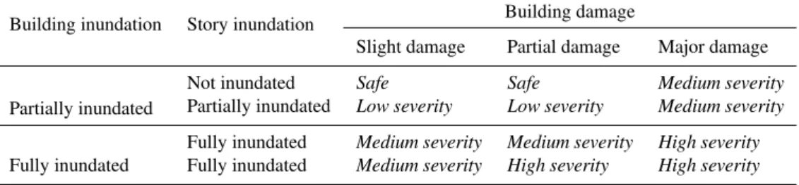
Flood severity is a parameter to evaluate the flood strength and the resistance of the buildings. Flood severity is di-vided into four levels: safe, low, medium and high, depend-ing on the builddepend-ing damage and builddepend-ing inundation. Build-ing damage is determined accordBuild-ing to the criteria of RESC-DAM (2000) as shown in Table 2. The whole building is fully inundated if the water depth is greater than the height of the building. Based on the concepts of building damage and building inundation, the flood severity in this study is defined in a matrix form in Table 3.

The loss of life in each flood severity zone is obtained with separate methods. In a safe zone, where no flood has arrived and the buildings are stable, the fatality rate is set as zero. In a high severity zone, as the buildings are either fully in-undated or totally damaged, the fatality is very high. Histor-ical records show that the average fatality rate in high sever-ity zones is 0.91 (Peng and Zhang, 2012a). Jonkman (2007) found that a logarithmic function fits the relationship be-tween fatality rate and water depth well. Thus, the fatality rates in medium and low severity zones are assumed to fol-low lognormal functions of water depth (h). Based on re-sults of regression analysis, the means and standard devi-ations of ln(h) are 1.65 and 0.56 for medium flood sever-ity and 3.38 and 1.19 for low flood seversever-ity, respectively (Peng and Zhang, 2012a). For example, the fatality rate of

the non-evacuated people in a low flood severity area (the buildings are neither seriously damaged nor fully inundated) is 10 % if the water depth is 6.4 m.

5.2 Modifications to HURAM

HURAM is implemented in Hugin Lite (Hugin Expert A/S, 2004), which is a program for the analysis of Bayesian net-works. Hugin Lite is powerful for the analysis of Bayesian networks involving discrete variables or continuous normal variates. However, in the dynamic decision making frame-work (DYDEM), the parameters are not limited to these two types. Thus, the calculations for flood consequence in DY-DEM are coded in Visual Basic in Microsoft Excel with Monte Carlo simulations instead of in Hugin Lite. The mod-ifications are summarized as follows, and details of the HU-RAM model are described by Peng and Zhang (2012a, b):

1. In HURAM, the parameter of time of day, with the states of 08:00–17:00, 17:00–22:00 and 22:00–08:00, is considered in the evacuation and sheltering compo-nents. In each state of time of day, the distributions of warning transmitting time (Tt), response time (St)and evacuation time (Et)are different. These can be handled as the lead time in HURAM is on the order of minutes to hours (the lead time is often in one state of time of a day). However, in DYDEM, the lead time for decision making is often on the order of days. The distributions of Tt,St andEt would be complicated if the time of day is considered. Thus, the effect of time of day is not considered in DYDEM.

2. In HURAM, the warning transmitting distributions are

W(3.5, 0.6),W(2.0, 0.5), andW(1.3, 0.7) for times of a day of 08:00–17:00, 17:00–22:00 and 22:00–08:00, re-spectively. HereW (a,b)denotes a Weibull distribution with coefficientsaandb:

Pt=1−exp(−atb). (41)

In DYDEM, we useW(1.3, 0.7) only for convenience and safety. W(1.3, 0.7) is suggested for moderately rapid warning by Lindell et al. (2002).

3. The response time distribution is assumed as W(4, 1) for emergent dam break situations in HURAM, with a mean value of 15 min and a standard deviation of 15 min. However, for decision making in DYDEM, the response time should be much longer as people need time to evacuate properties and prepare to live outside of their homes for several days. A distribution ofW(0.085, 2.55) is used according to practices of hurricane evacu-ation (Lindell et al., 2004).

5.3 Estimation of the flood consequences

Table 2.Recommended damage parameters for building structures (after RESCDAM, 2000).

Building type Partial damage Major damage

Unanchored wood-framed DV≥2 m2s−1 DV≥3 m2s−1 Anchored wood-framed DV≥3 m2s−1 DV≥7 m2s−1

Masonry, concrete and brick DV≥3 m2s−1_{andV≥2 m s}−1 _{DV≥7 m}2_s−1_{andV≥2 m s}−1

Table 3.Flood severity matrix.

Building inundation Story inundation Building damage

Slight damage Partial damage Major damage

Partially inundated

Not inundated Safe Safe Medium severity

Partially inundated Low severity Low severity Medium severity

Fully inundated Medium severity Medium severity High severity

Fully inundated Fully inundated Medium severity High severity High severity

and arranging the people at risk and necessary services (e.g. security and medical care). The initial costs are generally proportional to the number of people to be evacuated and the time interrupted (warning time):

C_i=cP_eva(PAR)(Wt+3) (42)

wherecis the expense per person per day (e.g. RMB 60 or US$ 9.5 per person per day); P_eva is the proportion of the people evacuated, which is estimated using the modified HU-RAM; Wt is the warning time in days. The 3-day time is taken as the minimal period of time between the predicted moment of flooding and the return of the residents (Frieser, 2004). The GDP interruption (CGDP)is calculated as

CGDP=

GDPP

365 (PAR)(Wt+4) (43)

where GDPPis the average GDP per person in the flood area.

It is expected that economic sectors need time to restart their business (Frieser, 2004). Therefore, a duration of 4 days is added to the warning time. Thus the evacuation costs (C)are given by

C=Ci+CGDP. (44)

The flood damage (D)is limited to the moveable properties in this study. The moveable properties are generally propor-tional to the number of people who have neither evacuated nor sheltered in safe zones:

D=(1−Peva)(1−Psafe)(PAR)αIp (45)

wherePsafe is the ratio of the people taking shelter in safe

zones; α is the proportion of properties that can be trans-ferred (0.1 is assumed);Ip is the property of each person,

which is taken as the cumulative net income (i.e. income mi-nus spending) per person:

Ip=(I−S)n (46)

whereI andSare the average income and spending per per-son;nis the average working period per person (e.g. 20 yr).

Despite ethical considerations, a human life has to be mea-sured for evacuation decision making. Jonkman (2007) re-viewed approaches of evaluating the human life. A method with macroeconomic considerations is chosen in this study (Van Manen and Vrijling, 1996, quoted by Jonkman, 2007). In this method, the value of a human life (VL)is given as

the product of GDP per person (GDPP) and the average

longevity (L):

VL=(GDPp)L. (47)

For example, the GDPP andL in Mianyang, China, are

RMB 13 745 and 75 yr in 2008 (Mianyang Bureau of Statis-tics, 2009). Thus, the value of one person in 2010 in China is RMB 1.03 million. The monetized loss of life (ML)is then

calculated as

M_L=V_L(LOL) (48)

where LOL is the loss of life predicted with HURAM as a function of warning time. AsPeva,Psafeand LOL can be

pre-dicted as functions of warning time with HURAM, the three categories of flood consequences are expressed as functions of warning time.

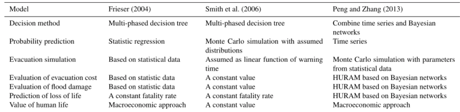
6 Dynamic decision making and comparison with existing methods

Table 4.Comparison of decision-making methods for dam break floods.

Model Frieser (2004) Smith et al. (2006) Peng and Zhang (2013)

Decision method Multi-phased decision tree Multi-phased decision tree Combine time series and Bayesian

networks

Probability prediction Statistic regression Monte Carlo simulation with assumed

distributions

Time series

Evacuation simulation Based on statistical data Assumed as linear function of warning

time

Monte Carlo simulation with parameters from statistical data

Evaluation of evacuation cost Based on statistic data A constant value HURAM based on Bayesian networks

Evaluation of flood damage Based on statistic data A constant value HURAM based on Bayesian networks

Prediction of loss of life A constant fatality rate A constant fatality rate HURAM based on Bayesian networks

Value of human life Macroeconomic approach A constant value Macroeconomic approach

to reduce the uncertainties in the model parameters. These will be presented with a specific dam-break case study in the companion paper (Peng and Zhang, 2013).

Frieser (2004) and Smith et al. (2006) published decision-making methods for floods with multi-phase decision trees, which are extended from the two-phase decision tree shown in Fig. 1. The time of possible flood occurrence is set as a target time (e.g. with enough lead time to evacuate the peo-ple) or the time achieving the worst predicted situation (e.g. highest water level or largest flood flow rate). The minimum expected total loss in each phase is obtained by comparing those in all alternatives. The optimal time to evacuate the PAR is the time achieving the minimum expected total loss.

Table 4 shows a comparison of these two methods and DY-DEM. Compared to the existing methods with decision trees, the dynamic decision framework suggested in this paper has several distinct features:

1. The framework takes the dam-failure probability as a time series and the flood consequences as functions of warning time. The time effects on both dam-break prob-ability and consequence are sufficiently considered. 2. Decision trees have a premise of a fixed occurrence

time, which may not be reasonable, as the probability of disaster occurrence is a stochastic process. The loss of life and properties may be underestimated if the flood occurs before the predicted moment, and vice versa. The dam-failure probability is simulated as a time series in DYDEM, in which the dam may break at any future time with a certain probability.

3. A successful evacuation can be attained when the avail-able time (i.e. the sum of warning time and flood rise time) is more than the demanded time (i.e. the sum of warning transmitting time, response time and evacua-tion time). The parameter distribuevacua-tions are based on ex-cising models and statistical data. Monte Carlo simu-lation is used to simulate the evacuation process with these parameter distributions.

4. The human risk or loss of life, which is complex and of-ten assumed as constant values in the existing methods,

is simulated with HURAM based on Bayesian net-works. Fourteen uncertain parameters and their inter-relationships are considered in this model.

5. Flood consequences, including evacuation cost, flood damage and loss of life, are closely related to evacua-tion rate (the proporevacua-tion of the people evacuated), shel-tering rate (the proportion of the people sheltered) and fatality rate (the proportion of the people who die). The processes of evacuation, sheltering and loss of life are simulated in HURAM with a Bayesian network.

7 Conclusions

Evacuation can save human life and properties but incurs costs at the same time. This paper presents a new framework of dynamic decision making for dam-break emergency man-agement. The following conclusions can be drawn:

1. The new framework presented in this paper takes the dam-failure probability as a time series and the flood consequences as functions of warning time. The as-sumption of a fixed flood occurrence time in a tradi-tional decision tree can be relaxed.

2. Overtopping failure occurs when the reservoir water volume exceeds the capacity. The inflow rates and reser-voir volumes are considered as stochastic processes and forecasted using time series in four steps: model iden-tification, model estimation, model diagnostic checking and forecasting. The probability of overtopping failure is predicted using the forecasted mean values and stan-dard deviations of the reservoir volume.

4. The total risk given a warning time is calculated consid-ering the probability of dam failure, evacuation costs, flood damage and loss of life, and the optimal warn-ing time to achieve a minimum total loss can be deter-mined. The PAR needs to be evacuated immediately if the calculated optimal warning time is close to the ini-tial time (t0); no warning is needed if the calculated

op-timal warning time is equal to the end of the study pe-riod (tend); the PAR should be evacuated at the optimal

time (top)with the minimum expected total loss if top

is betweent0 andtend. The decision can be delayed to

collect more information and reduce the uncertainties in the information. A delayed decision analysis can be per-formed with the updated information in this framework. A specific dam-break case study will be presented in the companion paper.

Appendix A

Time series models for forecasting inflow rate

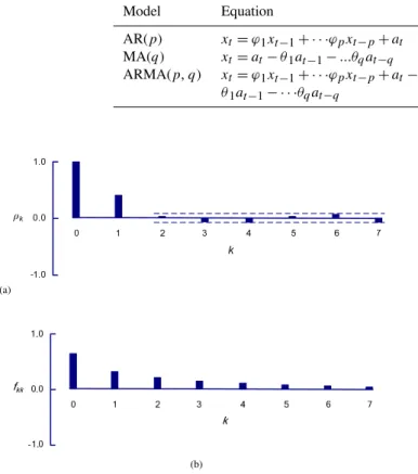
A stationary time series, which is one with its mean and variance independent of time, can usually be simulated as a mixed autoregressive–moving average (ARMA) model. In an ARMA model, a time-related variablextcan be expressed as a finite, linear aggregate of previous values of the time se-ries and random shocks,at,at−1,. . . ,at−q.

xt=ϕ1xt−1+ϕ2xt−2+ · · · +ϕpxt−p+at

−θ1at−1−θ2at−2− · · · −θqat−q (A1)

in whichϕ_i andθ_i are the coefficients of the ARMA(p, q)

model to be quantified. A random shock,at, is an indepen-dently and identically distributed (IID) stochastic process. Normallyat can be assumed as a normal distribution with a mean value of zero,N (0, σ_a2).

If a time series is not a stationary model, it can often be transferred to a stationary one by differentiating it (Box et al., 2008). A difference equation1xt is defined as

1xt=xt−xt−1 (A2)

and1dxtas

1dxt =1d−1xt−1d−1xt−1. (A3)

Ifxt can be transferred to a stationary time seriesωt with difference equation, namely,

ωt=1dxt=ϕ1ωt−1+ϕ2ωt−2+ · · ·+

ϕpωt−p+at−θ1at−1−θ2at−2− · · · −θqat−q, (A4) thenxt is called an autoregressive integrated moving average time series, or ARIMA (p, d, q). Actually, ARMA (p, q)is a special case of ARIMA (p, d, q)withd=0.

For an ARMA(p, q)model as shown in Eq. (A1), ifq=0, then

xt =ϕ1xt−1+ϕ2xt−2+ · · · +ϕpxt−p+at (A5) is called anautoregressivemodel of orderp, or AR(p)for short. If thep=0 in an ARMA(p, q)model, thenxtcan be expressed as a finite weighted sum ofat,at−1,. . . ,at−q:

xt =at−θ1at−1−θ2at−2− · · · −θqat−q, (A6) and is called amoving averagemodel of orderq, or MA(q)

for short.

A1 Model identification

The objective of model identification is to find a suitable time series model with orders (p, d, q)to simulate the observa-tions of a time series. For a given observed time series, the first step is to check whether it is stationary or not. If it is non-stationary, we need to transform it using Eq. (A3) until it becomes a stationary time series. The symptom of a non-stationary time series is that the autocorrelation functionρk at time lagkwill not die out quickly and will fall off slowly and nearly linearly with the increase ofk(Box et al., 2008). The autocorrelation function,ρk, is given by

ρk=

γk

γ0

(A7) whereγ is called aautocovarianceat time lagkand given by

γk=cov[xt, xt+k] =E[(xt−µ)(xt+k−µ)]. (A8) For a given time series of inflow rate,x1,x2, . . .xN, the

estimate ofγkis given by

γ_k∗= 1 N

NX−k

t=1

[(xt− ¯x)(xt+k− ¯x)] k=0,1, ..., N−1, (A9)

wherex¯is the average value of the observations ofxt. Another important parameter for a time series is its partial autocorrelation functionϕkk. Thej-th autocorrelation func-tionρj can be described as an autoregressive function as

ρj=ϕk1ρj−1+ϕk2ρj−2+ · · ·ϕk(k−1)ρj−k+1

+ϕkkρj−k j=1,2, ..., k (A10)

where the last coefficientϕkkis called a “partial autocorrela-tion funcautocorrela-tion”.ϕkkcan be estimated using a recursive formu-las (Durbin, 1960; Box et al., 2008).

Table A1.Identification of time series.

Model Equation Behaviour ofρk Behaviour ofϕkk

AR(p) xt=ϕ1xt−1+ · · ·ϕpxt−p+at Tail off Cut off atϕpp MA(q) xt=at−θ1at−1−...θqat−q Cut off atρq Tail off ARMA(p,q) xt=ϕ1xt−1+ · · ·ϕpxt−p+at−

θ₁at−1− · · ·θqat−q

Tail off Tail off

(a)

(b)

Fig. A1.Parameters of an assumed time series:(a)autocorrelation function,(b)partial autocorrelation function.

ϕkkhas a cutoff after lagp. Conversely, for MA(q), the auto-correlation functionρkcuts off after lagp, while its autocor-relation functionϕkktails off. If bothρkandϕkktail off, then a mixed process is suggested as shown in Table A1. For ex-ample, the autocorrelation function (ρk)and partial autocor-relation function (ϕkk)of an assumed time series are shown in Fig. A1. Asρkhas a cutoff after lag 1 andϕkktails off, the time series can be assumed as Ma(1). The assumption needs to be tested, which will be introduced later.

A2 Model estimation and diagnostic checking

An ARMA(p, q) time series, shown in Eq. (A1), has (p+ q+1) parameters, namely,ϕ1, ...,ϕp,θ1, ...,θq, andσa. The objective of model estimation is to find proper parameters to fit the observations of the time series. The error of a ARMA (p,q)time series at timetis expressed as

at=xt−ϕ1xt−1−ϕ2xt−2− · · · −ϕpxt−p

+θ1at−1+θ2at−2+ · · · +θqat−q. (A11) The least squares method is used to find parametersϕiandθi

for achieving the least sum of the squares ofat:

Min[

n

X

t=1

a_t2(ϕi, θi)], i=1,2, ..., n. (A12)

This can be implemented using a solver in Microsoft Ex-cel.

After obtaining the parameters, the next step is to conduct model diagnostic checking to make sure the assumed model is suitable. Box et al. (2008) show that the equation

n

K

X

k=1

[ρ_k∗(a)]2 (A13)

approximately follows aχ2(K−p−q)distribution, where

ρ_k∗(a)is the estimated autocorrelation function ofat, which is defined in Eqs. (A7) and (A8). The model can be checked through aχ2goodness-of-fit test at a confidence level (e.g. 5 % or 10 %).

Acknowledgements. The research reported in this paper was

substantially supported by the Natural Science Foundation of China (No. 51129902) and the National Basic Research Program (973 Program) (No. 2011CB013506).

Edited by: D. Keefer

Reviewed by: J.-J. Dong and H. Huang

References

ANCOLD: Guidelines on Risk Assessment. Working Group on Risk Assessment, Australian National Committee on Large Dams, Sydney, New South Wales, Australia, 1998.

BC Hydro: Guidelines for Consequence-Based Dam Safety Eval-uations and Improvements. Hydroelectric Engineering Division Report No. H2528, BC Hydro, Burnaby, BC, Canada, 1993. Box, G. E. P., Jenkins, G. M., and Reinsel, G. C.: Time series

anal-ysis: forecasting and control. Wiley Series in Probability and Statistics, Hoboken, New Jersey, USA, 2008.

Brockwell, P. J. and Davids, R. A.: Introduction to time series and forecasting, Springer Texts in Statistics, New York, USA, 1996. Chang, D. S. and Zhang, L. M.: Simulation of the erosion process

of landslide dams due to overtopping considering variations in soil erodibility along depth, Nat. Hazards Earth Syst. Sci., 10, 933–946, doi:10.5194/nhess-10-933-2010, 2010.

Durbin, J.: The fitting of time-series models, Rev. Int. Stat. Inst., 28, 233–244, 1960.

FEMA (Federal Emergency Management Agency): Federal guide-lines for dam safety – Hazard potential classification system for dams, Federal Emergency Management Agency, Washington DC, USA, 2004.

Frieser, B.: Probabilistic evacuation decision model for river floods in the Netherlands, Final report, Delft University of Technology, Delft, Netherlands, 138 pp., 2004.

Graham, W. J.: A procedure for estimating loss of life caused by dam failure. US Bureau of Reclamation, Dam Safety Office, Denver, USA, Report no. DSO-99-06, 44 pp., 1999.

Hugin Expert A/S: Hugin Lite, available at: http://www.hugin.com/ Products Services/Products/Demo/Lite/ (last access: 20 Jan-uary 2009), 2004.

Hydrologic Engineering Center (HEC): HEC-RAS, River Analysis System, hydraulic reference manual, version 4.0, developed by Hydrologic Engineering Center of US Army Corps of Engineers, Washington DC, USA, 2008.

Jonkman, S. N.: Loss of life estimation in flood risk assessment: theory and applications, Ph.D. Thesis, Delft University of Tech-nology, Delft, Netherlands, 2007.

Lindell, M. K., Prater, C. S., Perry, R. W., and Wu, J. Y.: EMBLEM: An Empirically Based Large Scale Evacuation Time Estimate Model, Texas A&M University Hazard Reduction & Recovery Center, College Station, Texas, USA, 2002.

Lindell, M. K., Prater, C. S., and Peacock, W. G.: Organizational communication and decision making for hurricane emergencies, Nat. Hazards Rev., 8, 50–60, 2007.

Liu, Y.: An explicit risk-based approach for large-levee safety deci-sions, MPhil thesis, The Hong Kong University of Science and Technology, Hong Kong, 2009.

Mianyang Bureau of Statistics: Report on the national economy and society development on Miangyang City in 2008. Mi-anyang Bureau of Statistics, Sichuan Province, China, available at: http://my.gov.cn/bmwz/942947769050464256/20090325/ 391646.html, last access: 25 March 2009.

Nielsen, N. M., Hartford, D. N. D., and MacDonald, J. J.: Selection of tolerable risk criteria for dam safety decision making, Proc. 1994 Canadian Dam Safety Conference, Winnipeg, Manitoba, Vancouver, BiTech Publishers, 355–369, 1994.

Peng, M. and Zhang, L. M.: Analysis of human risks due to dam break floods – part 1: A new model based on Bayesian networks, Nat. Hazards, 64, 1899–1923, 2012a.

Peng, M. and Zhang, L. M.: Analysis of human risk due to dam break floods – part 2: Application to Tangjiashan Landslide Dam failure, Nat. Hazards, 64, 903–933, 2012b.

Peng, M. and Zhang, L. M.: Breaching parameters of landslide dams, Landslides, 9, 13–31, 2012c.

Peng, M. and Zhang, L. M.: Dynamic decision making for dam-break emergency management – Part 2: Application to Tangji-ashan landslide dam failure, Nat. Hazards Earth Syst. Sci., 13, 439–454, doi:10.5194/nhess-13-439-2013, 2013.

RESCDAM: The use of physical models in dam-break flood anal-ysis: Rescue actions based on dam-break flood analysis, Final report of Helsinki University of Technology, Helsinki, Finland, 57 pp., 2000.

Smith, P. J., Kojiri, T., and Sekii, K.: Risk-based flood evacuation decision using a distributed rainfall-runoff model, Ann. Disas. Prev. Res. Inst., Kyoto Univ., No. 49B, 2006.

Urbina, E. and Wolshon, B.: National review of hurricane evacua-tion plans and policies: a comparison and contrast of state prac-tices, Transport. Res. Part A: Policy and Practice, 37, 257–275, 2003.

USBR (US Bureau of Reclamation): Guidelines for Achieving Pub-lic Protection in Dam Safety Decision Making, Dam Safety Of-fice, US Bureau of Reclamation, Denver, CO, USA, 1997. Van Manen, S. E. and Vrijling, J. K.: The problem of the valuation

of a human life. proceedings of ESREL 96 – PSAM III Confer-ence, Crete, Greece, 1996.

Woo, G.: Probabilistic criteria for volcano evacuation decisions, Nat. Hazards, 45, 87–97, 2008.

Xu, Y. and Zhang, L. M.: Breaching parameters of earth and rockfill dams, J. Geotech. Geoenviron. Eng., 135, 1957–1970, 2009. Zhang, L. M., Xu, Y., and Jia, J. S.: Analysis of earth dam failures-A