www.scielo.br/cam
Sources of uncertainty and error in the
simulation of
fl
ow in porous media
JAMES GLIMM1, SHULING HOU2, YOON-HA LEE1 DAVID H. SHARP3 and KENNY YE1
1Department of Applied Mathematics and Statistics
SUNY at Stony Brook, Stony Brook NY 11794-3600
2Theoretical Division, Los Alamos National Laboratory, Los Alamos, NM 87545 3Applied Physics Division and Theoretical Division
Los Alamos National Laboratory, Los Alamos, NM 87545
E-mail: [email protected] / [email protected]
Abstract. We are concerned here with the analysis and partition of uncertainty into component pieces, for a model prediction problem for flow in porous media.
Mathematical subject classification: 60H30, 62P30, 35R60.
Key words:uncertainty, solution error, porous media.
1 Introduction
In previous papers we have developed a Bayesian approach to uncertainty quan-tification [8, 9, 10] and the analysis of errors [5, 4, 6, 3, 2, 7] in numerical simulations. Prediction depends on both inverse and forward solutions, the for-mer to fix the model and its parameters and the latter to solve the model and make predictions. In the Bayesian framework, the indeterminacy potentially in-herent in the inverse solution is resolved by the use of a probability framework. In this framework, the probabilities of observation and solution errors are the leading contributions to the likelihood of an observation, which is a key factor in the definition of the posterior. The posterior is a probability distribution for models and parameters as constrained by observations. Both the inverse and the
forward steps depend on the forward simulation, errors in which introduce error and uncertainty into the analysis.
The purpose of this paper is to analyze and partition prediction uncertainty into component pieces associated with substeps of the prediction process. As with earlier papers, we illustrate our ideas with a simplified study of prediction for an idealized petroleum reservoir. We suppose that we have observations of oil production from an early time period (the “past”) and we use this information to constrain the prediction of the production for a later period (the “future”). The past production is known but the geology which gives rise to it is not. The errors or uncertainty in predictions of future production depend on geological, physical, and numerical parameters,e.g. the geology correlation length, the oil to water viscosity ratio, and the coarseness of the mesh used in simulating either the forward or inverse problems.
Our goal is model transparency. We want an uncertainty model, that is simple to describe in an understandable and plausible manner the separate contribu-tions to uncertainty, but accurate enough that it does not add to or increase the uncertainty being explained. Not only is such a model of benefit to the user. More importantly, such a model has a higher chance of being transferable from one problem to another. Because error models require extensive computation to validate and calibrate, the ability to transfer them (from a simple to a more realistic context) is important for the practical application of uncertainty analysis in general.
as distributed over the ensemble. The conventional 5%, 95% confidence intervals are then given as the mean prediction±1.96σ.
The main result of this paper is to estimate the separate contributions toσ. The observations are insufficient to specify the geology. As a result there is an inherent uncertainty in the problem specification. This contribution toσis labeledσgeology. In addition there is uncertainty associated with the use of approximate numerics to solve the inverse and forward problems, which we denote byσinverseandσforward. Finally, since we consider simplified (approximate) statistical methodologies, we introduce σstatistics to quantify the effects of these approximations. Use of finite sized ensembles and observational error introduce other uncertainties, not, considered here.
If the various sources of uncertainty were independent, then theσ would com-bine according to the rule
σtotal2 =
i
σi2 (1)
While this formula is useful qualitatively, we observe deviations from it in the range of 30% - 50%, indicating significant correlation among the different con-tributions to the uncertainty. We have been able to observe directly only some of the individualσi. For the others, some version of (1) is used to definethe
missingσi, tacitly assuming independence.
A second result is to determine the dependence of the variousσi on the
param-eters defining the problem. These paramparam-eters represent geological, numerical, and physical information (explanatory variables) which may be assumed to be known. Even in our simple study, the explanatory variables take on 60 distinct values in total. Thus it is important to compress and synthesize this information, so that useful and comprehensible trends in the dependence of the variousσ on the explanatory variables can be understood.
Finally, we observe a general ordering in the magnitudes of the variousσ:
σgeology≫σforward≫σinverse≫σstatistics (2)
2 The problem formulation
The present paper and earlier ones in this series [5, 4, 6, 3] serve to estab-lish a proto-type model for solution errors for flow in petroleum reservoirs. In order to focus on the uncertainty quantification issues, we have examined some-what idealized reservoir descriptions. The idealized Darcy and Buckley-Leverett equations
v= −K∇p; ∇ ·v=0
st +v· ∇f =0
are solved for a total seepage velocityvand oil saturations. HereK=K(x, z)is the random total permeability,the relative transmissivity andf the fractional flux. The permeabilityKis sampled from a lognormal distribution. The flow is nondimensionalized to lie in the unit square 0≤ x, z≤ 1. See also [4, 6] for a more detailed specification of the simulations.
The difference between the fine grid and the coarse grid solution is the solution error, which we study here. We only examine the oil cut, so the solution and the error are time series. We are not using actual production data in this study. We therefore model the real problem by selecting a particular geologyKi0as the
“correct” one, and consider the fine grid solution oil cutsi0 as a stand in for the
observed oil productionO.
We assume we have production data up to the present timeT0, defined in terms of an oil cut levelsi0(T0), here selected as 0.8, 0.6, or 0.4. For each choice of
horizontal correlation lengthλ50 geologies, sampled from a given log normal distribution, define the prior distributionP (K). According to Bayes theorem, the posteriorP (K|O)
P (K|O)= P (O|K)P (K)
P (O|K)P (K)dK .
P (K|O)is defined in terms of a likelihood,P (O|K), for the observationOto occur assuming the geologyKis correct. Letsf andscdenote the fine and coarse
(upscaled) solutions, respectively. As explained above, we choosesf,i0as a stand
in for an actual observationO. In evaluating the likelihood, we takeO =sf,i0
and compare tosc,j,j =i0. The likelihood is thus the probability of an error in
sc,j sufficient to produce the discrepancy
sf,i0(t )−sc,j(t ), 0≤t≤T0.
Since we assumeKj is correct in evaluating the likelihood, the likelihood
spec-ifies the probability of a solution error of a given size, to which we apply our Gaussian error model. See [4] for more detail.
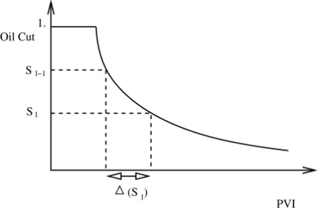
We specify the arrival time error model with five degrees of freedom. They are the breakthrough time and incremental elapsed time at oil cut levels of 0.8, 0.6, 0.4 and 0.2. To avoid an undue influence from numerical diffusion in the coarse grid simulations, we define the breakthrough time in terms of an oil cut value of 0.95. That is(Sl)=t (Sl)−t (Sl−1), where
t (Sl)=sup t
{s(t )≥Sl}, (3)
andSl =1−0.2·l, 0 ≤l≤N, and(S0)=t (S0). See the Fig. 1. Thus, the
a given change in the oil cut level for the fine and the coarse grid solutions. The mean and covariance matrix of the error are estimated by
e(l)= 1
n
i
ei(l) (4)
Cs(l, m)= 1
n−1
i
ei(l)−e(l)
ei(m)−e(m)
(5)
This elapsed time error model is used only to model the past,t ≤ T0, while future oil production
final time
present
si(t )dt (6)
is used to describe the future. The final time is set at 1.4 (PVI) in (6) andsimight
denote the fine or coarse grid solution. We correct the course grid solution for the mean solution error in all of its uses.
1.
(S ) S
S l−1
l
l
PVI Oil Cut
Figure 1 – Definition of the(Sl).
3 Findings
forward simulations. They are computed for each choice of exact geologyi0and then averaged (RMS) overi0to yield a final value.
This method is not applicable for fine grid solutions. For the fine grids, we specify an arrival time window (size 0.03) for past observations of the oil cut. Simulations passing through this window define the posterior.
3.1 Approximate independence of distinct error sources
We make precise the definitions of the different σi which will enter into our
analysis. σgeologyrepresents the uncertainty inherent in the prediction problem. σgeology originates in the incomplete set of observations (the oil cut) used to characterize the reservoir. It is defined as the standard deviation associated with the following prediction problem: the posterior is determined by fine grid solutions, using the windowing method, while the future is also simulated using the fine grid. σforwardis defined as the standard deviation of the prediction error resulting from use of the upscaled solution operator for forward predictions, starting from a knowledge of the exact geology. σinverse, the uncertainty in the selection of the posterior distribution, i.e. the inverse problem, is not directly observable, so we define it in terms of an RMS difference
σBayes ff2 =σgeology2 +σinverse2 (7) whereσBayes ffis defined predictionσfor prediction based on the Bayesian poste-rior (e.g. course grid solutions for the inverse problem) and the fine grid solutions for the forward simulation. The statistical uncertainty is also not directly observ-able, and is defined in terms of an RMS difference
See [7] for details. For comparison with (1), we defineσBayes statas the standard deviation associated with the Bayesian prediction using a coarse grid for both the inverse and forward steps and an approximate statistical model for the solution error covariance.
Eq. (1) asserts that
σBayes stat2 ≈σtotal2 ≡σgeology2 +σforward2 +σinverse2 +σstat2 . (9) Eliminating the trivial combinations from this formula which collapse by defi-nition, we are asserting that
σBayes stat2 ≈σtotal2 ≡σBayes ff stat2 +σforward2 . (10) There are actually three versions of this formula, with the full statistics covariance (no approximations), the diagonal covariance and the parametric model diagonal covariance. The formula asserts independence of prediction errors associated with the inverse and forward (past and future) aspects of prediction.
To assess the accuracy of (10), we perform an RMS average over all explanatory parameter values ofσtotal as defined by the formula and ofσBayes stat as defined directly. We find that (10) explains about 2/3 of the value ofσtotalcompared to σBayes statin the sense of an RMS average of the dependence of both sides of the equation on the explanatory parameters.
3.2 Dependence of error on problem parameters
Here we develop a parametric model for the dependence of the variousσion the
explanatory variables. We propose a relation of the form
lnσi2=a0+ageologyxgeology+ameshxmesh+apxp (11)
Here thea’s are coefficients to be determined and the x’s represent values for the explanatory variables. Thusxmesh =x/DwhereDis the interwell spacing and x is the scaled up mesh spacing. Also xp is the natural logarithm of
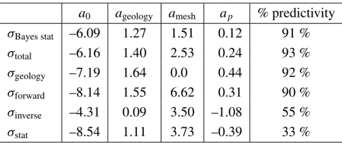
section is a table of thea’s for eachσi, together with a percentage of the RMS
parametric variability captured by this formula. The a’s are obtained from a nonlinear regression, to minimize errors in a fit to the exponential of (11). See Table 1.
a0 ageology amesh ap % predictivity
σBayes stat –6.09 1.27 1.51 0.12 91 % σtotal –6.16 1.40 2.53 0.24 93 % σgeology –7.19 1.64 0.0 0.44 92 % σforward –8.14 1.55 6.62 0.31 90 % σinverse –4.31 0.09 3.50 –1.08 55 % σstat –8.54 1.11 3.73 –0.39 33 %
Table 1 – Parametric model coefficients and RMS per cent predictivity of the model. The values given here utilize the parametric model for the diagonal approximation to the covariance to the error.
two approximations) are nearly identical, again showing that aσstator confidence interval inferred from this data will be very small.
5 10 20 40 0.2 0.4 0.6 0.8 1.00 0.05 0.1 ν λ
Figure 2 – Dependence ofσgeologyon viscosity ratioνand correlation lengthλ.
0.2 0.1 0.05 0.2 0.4 0.6 0.8 1.0 0 0.05 0.1 ∆x/D λ 0.2 0.1 0.05 0.2 0.4 0.6 0.8 1.0 0 0.05 0.1 ∆x/D λ 0.2 0.1 0.05 0.2 0.4 0.6 0.8 1.00 0.05 0.1 ∆x/D λ 0.2 0.1 0.05 0.2 0.4 0.6 0.8 1.00 0.05 0.1 ∆x/D λ
3.3 Ordering of error sources by magnitude
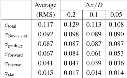
The main results of this section are summarized in Table 2, which justifies the ordering given in (2). Each entry is defined as an RMS average over the 60 explanatory parameter values, or over those values for fixedx.
Average x/D
(RMS) 0.2 0.1 0.05
σtotal 0.117 0.129 0.113 0.108 σBayes stat 0.092 0.098 0.089 0.090 σgeology 0.087 0.087 0.087 0.087 σforward 0.067 0.084 0.061 0.053 σinverse 0.041 0.047 0.039 0.036 σstat 0.015 0.017 0.014 0.014
Table 2 – Magnitudes of distinct contributions to the standard deviation for relative error in predictions. We tabulate in the first column the RMS average over all explanatory parameters, and in the next three columns the RMS average withxheld fixed.
4 Acknowledgments
James Glimm is supported by the MICS program of the U.S. Department of En-ergy DE-FG02-90ER25084, DE-AC02-98CH10886, grant DAAL-03-91-0027 and the National Science Foundation, grant DMS-01022480. Shuling Hou and David H. Sharp are supported by the U.S. Department of Energy. Yoon-ha Lee is supported by the Department of Energy DE-FG02-90ER25084.
REFERENCES
[1] M.A. Christie, T.C. Wallstrom, L.J. D.S. Hou, D.H. Sharp and Q. Zou,Effective medium boundary conditions in upscaling, in Proceedings of the 7th European Conference on the Mathematics of Oil Recovery, Baveno, Italy, Sept. 5-8 (2000).
[2] B. DeVolder, J. Glimm, J.W. Grove, Y. Kang, Y. Lee, K. Pao, D.H. Sharp and K. Ye,
Uncertainty quantification for multiscale simulations, Journal of Fluids Engineering,124
(2002), pp. 29–41.
[3] J. Glimm, Y. ha Lee, and K.Ye,A simple model for scale up error, Contemporary Mathematics,
[4] J. Glimm, S. Hou, H. Kim, Y. Lee, D. Sharp, K. Ye and Q. Zou,Risk management for petroleum reservoir production: A simulation-based study of prediction, J. Comp. Geo-sciences,5(2001), pp. 173–197.
[5] J. Glimm, S. Hou, H. Kim, D. Sharp and K. Ye,A probability model for errors in the numerical solutions of a partial differential equation, CFD Journal,9(2000).
[6] J. Glimm, S. Hou, Y. Lee, D. Sharp and K. Ye,Prediction of oil production with confidence intervals, SPE 66350, Society of Petroelum Engineers, (2001). SPE Reservoir Simulation Symposium held in Houston, Texas, 11-14 Feb.
[7] J. Glimm, S. Hou, Y. Lee, D. Sharp and K. Ye,Solution error models for uncertainty quantifi-cation, Contemporary Mathematics, (2003). Submitted. SUNYSB preprint 02-16. LANL preprint LA-UR: 02-5987.
[8] J. Glimm and D.H. Sharp,Stochastic partial differential equations: Selected applications in continuum physics, in Stochastic Partial Differential Equations: Six Perspectives, R.A. Carmona and B.L. Rozovskii, eds., Mathematical Surveys and Monographs, American Math-ematical Society, Providence, (1997).
[9] J. Glimm and D.H. Sharp,Stochastic methods for the prediction of complex multiscale phe-nomena, Quarterly J. Appl. Math.,56(1998), pp. 741–765.
[10] J. Glimm and D.H. Sharp,Prediction and the quantification of uncertainty, Physica D,
133(1999), pp. 152–170.
[11] T. Wallstrom, M.A. Christie, L.J. Durlofsky and D.H. Sharp, Effective flux boundary conditions for up scaling porous media equations, Transport in Porous Media,46(2000), pp. 139–153.
[12] T. Wallstrom, S. Hou, M.A. Christie, L.J. Durlofsky and D.H. Sharp,Accurate scale up of two phase flow using renormalization and nonuniform coarsening, Computational Geoscience,
3(1999), pp. 69–87.
[13] T. Wallstrom, S. Hou, M.A. Christie, L.J. Durlofsky and D.H. Sharp,Application of a new two-phase upscaling technique to realistic reservoir cross sections, Proceedings of the SPE 15th Symposium on Reservoir Simulation, (1999), pp. 451–462. SPE 51939.