www.scielo.br/cam
Fluid-solid mixtures and electrochemomechanics:
the simplicity of Lagrangian mixture theory
JACQUES M. HUYGHE, R. VAN LOON and F.T.P. BAAIJENS
Department of Biomedical Engineering, Eindhoven University of Technology Eindhoven, The Netherlands
E-mail: [email protected]
Abstract. Today, the focus of physical scientists is shifting more to biology than ever before. A biological tissue is typically an ionised porous medium saturated with a solution of ions and neutral solutes. Because classical porous media theories do not account for ionisation, the present paper addresses this issue. The characteristic pore size in most biological applications is close to the molecular level and hence below the Debye-Hueckel scale. Not only pressure gradients and concentration gradients, but electrical gradients as well are intimately linked to fluid flow, ion flow and deformation.
Mathematical subject classification: 76ZXX, 76W05, 76S05.
Key words:swelling, shale, cartilage, finite deformation, equipresence.
1 Introduction
Since antiquity, the phenomenon of swelling of tissues has been closely related to health and disease. Biological, synthetic and mineral porous media often ex-hibit swelling or shrinking when in contact with changing salt concentrations. This phenomenon, observed in clays, shales, cartilage and gels, is caused by a combination of electrostatic forces and hydration forces [11]. In case of biolog-ical tissue, electrostatic forces are often dominant. Classbiolog-ical concepts, such as the transmembrane potential of cells are directly associated with these electro-static forces. Already years ago, Biot understood that his theories were closely associated with transmembrane phenomena in living cells [4]. At least four
components are involved in the swelling mechanics: a solid, a fluid, anions and cations. Lai et al. [11] developed a triphasic theory for soft hydrated tissue and applied the theory to cartilage while neglecting geometric non-linearities. They verified the theory for one-dimensional equilibrium results. As soft tissues and cells are commonly subject to large deformations, our group developed a finite deformation theory of ionised media [9]. In order to simplify the mathemetics as much as possible a Lagrangian form of the entropy inequality has been derived which leads to equations consistent with Biot’s porous media theories in a more straightforward way than the more familiar Eulerian approach of Bowen [6]. The incompressibility and electroneutrality conditions are introduced by means of two Lagrange multipliers; the latter is physically interpreted as an electrical potential, the former as a pressure.
2 Fluid-solid mixtures
We shall derive equations applicable to the behaviour of elastic incompressible fluid saturated porous media from mixture theory.
2.1 Assumptions
We consider the porous medium as a two-component mixture, composed of a solid (superscripts) and a fluid component (superscriptf). Saturation requires:
ϕs +ϕf =1. (1)
We assume that no mass-exchange occurs between the components. Each com-ponent is assumed incompressible:
ρiα = ρ α
ϕα =constant, α =s, f. (2)
2.2 Conservation laws 2.2.1 Conservation of mass
In the absence of mass exchange the local law of conservation of mass of com-ponentαreduces to:
∂ρα
∂t + ∇∇∇ · (ρ
αvα)=0, α=s, f. (3)
We can rewrite (3):
∂ϕα
∂t + ∇∇∇ · (ϕ
αvα)=0, α=s, f. (4)
Summation of the equations (4) yields the local mass balance of the mixture:
∇∇∇ · (ϕsvs)+ ∇∇ ·∇ (ϕfvf)=0, (5)
or:
∇∇∇ · vs+ ∇∇∇ ·
ϕf(vf −vs)=0. (6)
The first term of (6) represents the rate of volume increase of a unit volume of mixture. The second term represents the fluid flux from this unit volume. Eq. (6) states that every volume-increase or decrease of the mixture is associated with an equal amount of in- or outflux of liquid. At this point it is useful to refer current descriptors of the mixture with respect to an initial state of the porous solid. As is usual in continuum mechanics, we define the deformation gradient tensorF mapping an infinitesimal material line segment in the initial state onto the corresponding infinitesimal line segment in the current state. The relative volume change from the initial to the current state is the determinant of the deformation gradient tensorJ =detF. If we introduce volume fractions
α =J ϕα (7)
per unit initial volume, we can rewrite the mass balance equation (4) as follows:
Dsα
Dt +J∇∇∇ · [ϕ α
(vα−vs)] =0 (8)
when using the identity:
Ds
DtJ =J∇∇∇ · v
2.2.2 Conservation of momentum
Considering the assumptions stated earlier, momentum balance reduces to:
∇∇∇ · (σα)c+ ˆpα =0, α =s, f. (10)
The momentum interactionpˆα arises e.g., as a consequence of friction between the fluid and the solid. We assume no moment of momentum interaction between fluid and solid. Therefore we tacitly assumed the symmetry of the partial Cauchy stress tensor in (10). Summation of the equations (10) yields the local momentum balance for the mixture as a whole:
∇ ∇
∇ · σs+ ∇∇∇ · σf = ∇∇∇ · σ =0, (11)
if we use:
ˆ
ps + ˆpf =0. (12)
2.2.3 The entropy inequality
The local form of the entropy inequality applied to the mixture as a whole, reduces to:
α=s,f
−ραD αF˜α
Dt ˜
Fα +σα:Dα − ˆpα· uα
≥0. (13)
We introduce the strain energy function
W =J
α=s,f
ραF˜α =J α=s,f
ψα (14)
as the Helmholtz free energy of a mixture volume which in theinitialstate of the solid equals unity. ψα is the Helmholz free energy of constituentαper unit
mixture volume. Rewriting the inequality (13) for the entropy production per initial mixture volume – i.e. we multiply inequality (13) by the relative volume changeJ – we find:
−D s
DtW +Jσ: ∇∇∇v
s +J∇∇∇ ·
(vf −vs)· σf −(vf −vs)ψf
2.3 Constitutive restrictions
We use the entropy inequality to derive constitutive restrictions for the mixture. The entropy inequality should hold for an arbitrary state of the mixture, com-plying with the balance laws and with incompressibility. There are two ways to comply with these restrictions. One is substitution of the restriction into the in-equality, resulting in elimination of a field variable. The other is by introduction of a Lagrange multiplier. The mass balance of the mixture (6) is accounted for by means of a Lagrange multiplier. Other balance laws and the incompressibility conditions (2) are accounted for by means of substitution. From the inequality 15 we see that the apparent density and the momentum interactionpˆα is already eliminated from the inequality. In other words the conditions of incompressibil-ity and the momentum balance of the constituents have already been substituted into the second law. The divergence of the partial stress tensor of the solid∇∇∇ ·σs and the heat suppliesrα also are absent from 15. Thus the momentum balance
of the mixture and the energy balance have already been substituted in the sec-ond law. Therefore, restrictions still to be fulfilled are the mass balances of the constituents (3) and mass balance of the mixture (6). The latter is substituted by means of a Lagrange multiplierp:
−D s
DtW+Jσe: ∇∇∇v s +
J[σf +(pϕf −ψf)I] : ∇∇∇(vf −vs)
+J (vf −vs)· (−∇∇∇ψf +p∇∇∇ϕf + ∇∇∇ · σf)≥0.
(16)
in which the effective stressσeis defined as
σe =σ+pI (17)
2.3.1 Choice of independent and dependent variables
We choose as dependent variables the dynamic variables appearing in inequality 16: W, ψf, σe, σf +pϕfI,∇∇∇ · σf +p∇∇∇ϕf. Their number should equate
phenomena involved in the behaviour of the material. We choose as independent variables the kinematic variables: the Green strain of the solidEs, the fluid volume fractionf and the fluid velocity relative to the solid vf −vs. For
reasons of objectivity we need to transform all the vectors and tensors among the dependent and independent variables back to the initial state. This yields for the constitutive relationships:
W =W (Es, f,vf s),
ψf =ψf(Es, f,vf s),
σe =F · Se(Es, f,vf s)· Fc,
σf −ϕfpI =F · Sf(Es, f,vf s)· Fc
ˆ
pf −p∇∇∇ϕf =F · ˆPf(Es, f,vf s)
(18)
with
vf s =F−1· (vf −vs) (19)
The principle of equipresence requires that all dependent variables appear in each of the constitutive relationships. The choice of the independent variables is paramount for the form of the constitutive relationships that are derived. E.g., including for the solid Green strain only and no measure of strain rate, implies elasticity of the solid. In mixture mechanics it is also important to realise that each of the variables is an averaged value of a physical quantity over an averaging volume. It may seem surprising that the shear rate of the fluid is not included in the list of independent variables, although the viscosity of the fluid is absolutely essential for the behaviour of the mixture. The reason for this is that in a porous medium the shear rate at one side of the pore has a sign opposite to the shear rate at the other side of the pore. The expectation value of the shear rate in a representative elementary volume is therefore the shear rate of the solid, i.e. a generally very low value, not representative for the dissipation in the fluid. It is therefore more obvious to use the fluid velocity relative to the solid as a macroscopic measure of the microvalues of the shear rate. The fluid volume fractionf is not independent of the Green strain because of incompressibility:
Because of the strong non-linearity of equation (20), elimination of one of the variables is tedious. In fact, the way we deal with the interdependence of these two variables is by means of the Lagrange multiplier p. The condition (6) is in fact a differentated form of equation (20). This legitimises the use ofEsandf as independent variables.
2.3.2 Constitutive relationships
Applying the chain rule for time differentiation of W:
DsW
Dt =
∂W ∂Es:
DsEs
Dt +
∂W ∂f
Dsf
Dt +
∂W
∂vf s (21)
and substituting the mass balance of the constituents (8) for the elimination of
Dsf
Dt from the inequality 16:
Jσe−F · ∂W ∂E · F
c
: ∇∇∇vs + ∂W ∂vf s ·
Ds Dtv
f s
+J[σf +(µfϕf −ψf)I] : ∇∇∇(vf −vs)
+J (vf −vs)· (−∇∇∇ψf +µf∇∇∇ϕf + ∇∇∇ · σf)≥0.
(22)
in whichµf is the chemical potential of the fluid:
µf = ∂W
∂f +p (23)
Eq. (22) should be true for any value of the state variables. Close inspection of the choice of independent variables and the inequality (22), reveals that the first term of (22) is linear in the solid velocity gradient∇∇∇vs, the second term linear inDDtsvf s and the third term linear in the relative velocity gradients∇∇∇(vf −vs). Therefore, by a standard argument, we find:
σe =
1 JF ·
∂W ∂E · F
c (24)
∂W
∂vf s =0 (25)
leaving as inequality:
J (vf −vs)· (−∇∇∇ψf +µf∇∇∇ϕf + ∇∇∇ · σf)≥0. (27)
Eq. (24) indicates that the effective stress of the mixture can be derived from a strain energy function W which represents the free energy of the mixture. Eq. (25) shows that the strain energy function cannot depend on the relative velocity of fluid versus solid. This result – only obtained in a Lagrangian formulation – simplifies the constitutive laws to a large extent, because a vectorial variable disappears among the independent variables of the free energyW, and its deriva-tives, the effective stress and the chemical potential. The partial free energies, ψs andψf cannot be shown independent from the relative velocity. Thus, the effective stress of a biphasic medium can be derived from a regular strain energy function, which physically has the same meaning as in single phase media. Ac-cording to equation (26) the partial stress of the fluid is a scalar. Transforming the relative velocities to their Lagrangian equivalents, we find in stead of (27):
vf s ·
− ∇∇∇0ψf +µf∇∇∇0ϕf + ∇∇∇0· σf
≥0. (28)
in which∇∇∇0=Fc· ∇∇∇is the gradient operator with respect to the initial configura-tion. Note that asµf∇∇∇0ϕf+∇∇∇0·σfdepends onvf saccording to the constituive
relationships (18), the lefthandside of inequality (28) is not a linear function of vf sand therefore it is incorrect to equate the factor−∇∇∇0ψf+µf∇∇∇0ϕf+∇∇∇0·σf to zero. From a physical point of view it is obvious that unlike the elastic de-formation of the solid the flow of fluid relative the solid results in an entropy production. If we assume that the system is not too far from equilibrium, we can express the dissipation (28) associated with relative flow of fluid and ions as a quadratic function of the relative velocities:
−∇∇∇0ψf +µf∇∇∇0ϕf + ∇∇∇0· σf =B· vf s (29) Bis a semi-positive definite matrix of frictional coefficients. Substituting equa-tion (26) into equaequa-tion (29) yields the Lagrangian form of Darcy’s law:
−ϕf∇∇∇0µf =B· vf s (30)
2.4 Physical interpretation of the constitutive variables
The Lagrange multiplier p should be interpreted as the hydrostatic pressure in the fluid.
∇∇∇ · σe− ∇∇∇p=0. (31)
If we define the permeability tensorKas:
K =(ϕf)2B−1 (32)
equation (30) becomes:
ϕf(vf −vs)= −K· ∇∇∇ p+ ∂W ∂f
. (33)
Eq. (33) is the threedimensional form of Darcy’s law. The difference between the chemical potentialµf and the pressurepis thematricpotential. The matric potential accounts for adsorption and capillary forces. It can be quantified ex-perimentally using capillary rising heights. In Terzaghi’s consolidation theory the matric potentisal is neglected, not because it is negligible in absolute terms but because its gradient is negligible in an homogenous medium with limited variation of fluid volume fraction and coarse pore structure.
2.5 Resulting equations
The resulting equations are:
Momentum balance of the mixture:
∇ ∇
∇ · σe− ∇∇∇p=0 (34)
Mass balance of the mixture:
∇∇∇ · vs− ∇∇∇ · (ϕf(vf −vs))=0 (35)
Darcy’s law:
Stress-strain relationship:
σe=(detF)−1F· ∂W ∂Es · F
c
, (37)
Constitutive law for the chemical potential of the fluid:
µf =p+ ∂W
∂f (38)
The total stress in the mixture is composed of an effective stress and a hydro-dynamic pressure: σ = σe−pI. The effective stress σe is derived from the
strain energy function of the mixtureW. In equation (38)F is the deformation gradient tensor of the solid andEsthe Green strain tensor of the solid. The strain energyW in a function of the solid strainE.
Dynamic boundary conditions are:
[(σe−pI)· n] =0 (39)
withnthe outer normal along the boundary and the square brackets represent the difference between the value at either side of the boundary.
Vfµf
=0, (40)
with as a special case the evaporation boundary condition:
Vfµf =RT ln p d
pd s
(41)
is incompressible, the medium outside the boundary need not be incompressible as is the case for evaporation. Kinematic boundary conditions are:
[u] =0 (42)
[(vf −vs)·n] =0 (43)
3 Donnan Osmosis
When an ionised medium is in contact with a monovalent salt solution, diffusion of salt ions and flow of fluid take place between the medium and the salt solution until equilibrium is reached:
µ+ = µ+ (44)
µ− = µ− (45)
µf = µf (46)
µ+ is the electrochemical potential of the cations, µ− is the electrochemical potential of the anions andµf the chemical potential of the fluid in the medium. The corresponding overlined symbols refer to chemical potentials in the outer solution. Standard expressions for (electro)chemical potentials are found in the literature [15]. If we assume incompressibility for each constituent, i.e. same partial molar volumes in either solution, we find:
µ+=µ+0 + 1
V+(RT lna ++
F ξ ) (47)
µ−=µ−0 +
1
V−(RT lna −−
F ξ ) (48)
µf =µf0 +p+RT Vf
lnaf (49)
and (45) leads to:
a−a+ = a+a− (50)
ξ−ξ = RT
2F ln a−a+
a+a− (51)
whereξ−ξis the Donnan potential between the inner and outer solution. If we definecf cas the fixed charge density per unit fluid volume of the inner solution,
taken positive for positive charges and negative for negative charges, we can write the electroneutrality conditions as:
c− = c++cf c (52)
c−=c+=c (53)
c+ and c− are the cationic and anionic concentrations per unit fluid volume in the inner solution, while the corresponding overlined symbols pertain to the outer solution. In terms of the volume fractions introduced in equation (7), the concentrations are
cβ = β
fV¯β (54)
From the previous equations we derive the Donnan equilibrium concentration of the ions:
2c+ = −cf c+
(cf c)2+4f2c2 (55)
2c− = cf c+
(cf c)2+4f2c2 (56)
with
f2= f +
f−
f+f− (57)
andfβ = aβ
cβ, β = +,−the activity coefficient of componentβ. Equations
during swelling and for the associated osmotic pressureπ. Using equation (49) one can derive Van’t Hoff relation from (46):
π =p−p=RTŴf(c++c−)−2Ŵfc (58)
provided that the molar fractions of the ions are small compared to the molar fraction of the fluid.Ŵf andŴf are the osmotic coefficients.
4 Quadriphasic theory
It may be clear from the above considerations that physical phenomena occuring in the porous medium are a combination of mechanical, chemical and electrical effects. The interrelationship between these effects are well known for membrane processes [16]. The purpose of this paper is to generalise these relationships for porous media subjected to threedimensional finite deformation. The four phases that we consider in the medium are: solid (superscript s), fluid (superscript f), monovalent anions (superscript –) and monovalent cations (superscript +). As-suming all components intrinsically incompressible and excluding mass transfer between phases, the mass balance of each phase is given by (4), whereα takes the values s,f,+ or – . We assume saturation
ϕs+ϕf +ϕ++ϕ−=1. (59)
Summation of the equation (4) yields the mass balance of the mixture:
∇ · vs + f,+,−
∇ ·
ϕα(vα − vs)
=0 (60)
The electrostatic interactions are accounted for by means of an electroneutrality condition:
Ds Dt
β=f,+,− zββ
¯
Vβ =0 (61)
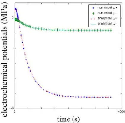
Figure 1 – Electrochemical potential of anions and cations as a function of time during swelling of a one dimensional ionised medium. The solution from a 3D finite element
code [17] is compared to the analytical solution [18].
Helmholz free energy of constituentαper unit mixture volume. The inequality for the entropy production per initial mixture volume reads:
−D s
DtW +Jσ: ∇ v s
+J∇ · β=f,+,−
(vβ − vs)· σβ −(vβ− vs)ψβ≥0. (62)
We assume the existence of a Lagrange multiplierpfor the saturation condition andλfor the electroneutrality condition. The entropy inequality transforms into:
−D s
DtW +Jσ
eff: ∇ vs
+J
β=f,+,−
σβ +
p+z βλ
Vβ
ϕβ−ψβ
I
: ∇(vβ − vs)
+J
β=f,+,−
(vβ − vs)·
− ∇ψβ+ p+z βλ
Vβ
∇ϕβ+ ∇ · σβ
in whichzβ is the valence of constituent β, σeff is the effective stress of the medium. We choose as independent variables the Green strainE, the Lagrangian form of the volume fractions of the fluid and the ionsβ, and of the relative
velocities vβs = F−1· (vβ − vs), β = f,+,−. We apply the principle of equipresence asd the chain rule for time differentiation ofW:
Jσeff −F · ∂W ∂E · F
c
: ∇ vs
+
β=f,+,−
∂W ∂vβs ·
Ds Dtv
βs+J
σβ+(µβϕβ−ψβ)I: ∇(vβ− vs)
+J (vβ− vs)· (− ∇ψβ +µβ∇ϕβ + ∇ · σβ)
≥0.
(64)
in whichµβ are the electrochemical potentials of fluid and ions:
µf = ∂W ∂f +p
µ+ = ∂W ∂+ +
λ
V+
+p (65)
µ− = ∂W ∂− −
λ
V− +p
By a standard argument [7], we find:
σeff = 1 JF ·
∂W ∂E · F
c (66)
∂W
∂vβs =0 (67)
σβ =(ψβ−µβϕβ)I (68)
leaving as inequality:
β=f,+,−
J (vβ− vs)·
− ∇ψβ +µβ∇ϕβ + ∇ · σβ
≥0. (69)
Equation (67) shows that, again, the strain energy function cannot depend on the relative velocities. In fact this result can easily be generalised to mixtures of arbitrary number of components. Thus, the effective stress of a quadriphasic medium can be derived from a regular strain energy function, which physically has the same meaning as in single phase or biphasic media, but which can depend on both strain and ion concentrations in the medium. According to equation (68) the partial stress of the fluid and the ions are scalars. Transforming the relative velocities to their Lagrangian equivalents, we find in stead of (69):
β=f,+,− vβs·
− ∇0ψβ +µβ∇0ϕβ+ ∇0· σβ≥0. (70)
in which∇0 = Fc· ∇ is the gradient operator with respect to the initial con-figuration. If we assume that the system is not too far from equilibrium, we can express the dissipation (70) associated with relative flow of fluid and ions as a quadratic function of the relative velocities:
− ∇0ψβ+µβ∇0ϕβ+ ∇0· σβ =
γ=f,+,−
Bβγ · vγ s (71)
Bβγ is a positive definite matrix of frictional tensors. Substituting equation (68) into equation (71) yields Lagrangian forms of the classical equations of irreversible thermodynamics:
−ϕβ∇0µβ =
γ=f,+,−
Bβγ · vγ s (72)
part of the energy function as
W (f, +, −)=µf0f +µ+0++µ−0− −RT Ŵ
+ ¯ V+ +
− ¯ V−
ln(f)+RT + ¯ V+ ln
+ ¯ V+ −1 +RT − ¯ V− ln
− ¯ V− −1 (73)
Hence the expressions 65, take the form:
µf = −RT Ŵ + fV¯+ +
− fV¯−
+p
µ+ = RT ln
+ (f)ŴV¯+ +
λ
V+
+p (74)
µ− = RT ln
− (f)ŴV¯− −
λ
V− +p
which is consistent with the classical expressions for electrochemical potentials (47-49), provided that we identify the activity of ionβ as
aβ =fβcβ = β
(f)ŴV¯β (75)
the activity coefficient as
fβ =(β)1−Ŵ (76)
and the Lagrange multiplierλas the product of the electrical potential and Fara-day constant:
λ=F ξ (77)
Equations (74-76) justifies the form of the mixing energy (73) as the mixing energy belonging to the Donnan osmosis model. Rearranging equation (65) yields,
µα −p− z α
¯ Vαλ=
β=f,+,−
in which,
Cαβ =
∂2W (f, +, −) ∂α∂β
−1 = ⎡ ⎢ ⎢ ⎢ ⎣ RT Ŵ + ¯
V+(f)2 +
− ¯ V−(f)2
− RT Ŵ ¯
V+f −
RT Ŵ ¯ V−f
−RT Ŵ ¯ V+f
RT ¯
V++ 0
−RT Ŵ ¯
V−f 0
RT ¯ V−−
⎤ ⎥ ⎥ ⎥ ⎦ −1 (79)
is the inverse of the Hessian of the mixing energy. To obtain the weak formulation the equations are multiplied by arbitrary, time independent weighing functions and integrated over the volume of the mixture (). The momentum equation is multiplied by a weighing functionwx. The saturation condition, mass equation
and equation for electroneutrality are multiplied by the weighing functionswp, wα
µandwξ, respectively. After partial integration and applying the divergence
theorem, we find,
⎧ ⎪ ⎪ ⎪ ⎪ ⎪ ⎪ ⎪ ⎪ ⎪ ⎪ ⎪ ⎪ ⎪ ⎪ ⎪ ⎪ ⎪ ⎪ ⎪ ⎪ ⎪ ⎪ ⎪ ⎨ ⎪ ⎪ ⎪ ⎪ ⎪ ⎪ ⎪ ⎪ ⎪ ⎪ ⎪ ⎪ ⎪ ⎪ ⎪ ⎪ ⎪ ⎪ ⎪ ⎪ ⎪ ⎪ ⎪ ⎩ ∇ wx
c
:σ d=
Ŵ
wx· (σ · n) dŴ ,
wp
∇ · vs
d− wp 1 J β
Dsβ
Dt d=0,
wµα
1 J
Dsβ
Dt d+
α
Kαβ∇µα
· ∇wµα d
=
Ŵ wαµ
α
Kαβ∇µα
· n dŴ ,
wξ ⎛ ⎝ 1 J β zβF
¯ Vβ
Dsβ Dt
⎞
⎠ d=0.
(80)
in which Ŵ is the outer surface of the medium and Kαβ = ϕαϕβ(Bαβ)−1 a
generalised diffusion-permeability tensor. We choose to use an updated Lagrange formulation. The total deformation tensorF may be divided into,
where Fn describes the deformation from the initial configuration 0 to the
reference configurationn, andFdenotes the deformation from the reference
configuration to the current state. When transforming the balance equations to a known domain, the reference configurationnis used. The gradient operator
is transformed according to,
∇ =F−c · ∇n (82)
As the total deformation is divided, the volume ratio is divided in a similar way. From the definition ofJ it follows that,
J =JJn (83)
Time discretization of the material time derivatives forJandβ yields,
J
∇ · vs
= ˙J=
J−1
t (84)
Dsβ
Dt =
β−β n
t (85)
For the mass balance a time discretization scheme is applied,
χ =θχ (t n+t )+(1−θ )χn (86)
The time discretization scheme can be varied easily from implicit Euler (θ =1) to explicit Euler (θ = 0). The Newton-Raphson iteration procedure is used to determine a sequence of approximate solutions of the non-linear equations. Quadratic interpolation functions(
∼)are used for the position field and weighing
functionww. Linear interpolation functions(
∼)are taken for the discretization
S −L 0 0 δ u
∼ −R∼
−LT − β
Cαβ Cαβ −
β Cαβz
αF
¯
Vα δp∼ U∼−
β Q ∼β
=
0 Cαβ −Kαβ−Cαβ Cαβz
αF
¯
Vα δµ∼
α Q
∼β+
α (T
∼1+T∼2)
0 −
β Cαβz
αF
¯
Vα Cαβ zαF
¯ Vα −
β zβF
¯ VβCαβ
zαF ¯
Vα δ ξ∼ −
α zαF
¯ VαQ∼α
S =
BT
DF +Dτ +DJ
B d
L =
B ∼w∼
T d
Cαβ =
α ∼ 1 JnJ
Cαβ ∼
T d
Kαβ = θ
α
BTµKαβBµt d
R ∼ =
BTσ
∼d U ∼ = ∼
J−1 J d T ∼1 = θ
BTµKαβBµt dµ ∼ α
T ∼2
= (1−θ )
1 J
BTµF KαβFTBµt dµ ∼ α ϕ Q ∼β = ∼ 1 JnJ
The matricesDF,Dτ andDJ result from the linearisation ofF,σeff andJ
respectively. The matricesB and Bµ contain the derivatives of the quadratic
and linear interpolation functions respectively. The columnBw
∼ also contains of
derivatives of the quadratic interpolation functions. For calculation a 27-node brick element is chosen with 3 displacements in every node. In each corner of the brick one pressure, 3 chemical potentials and an electric potential is calculated, resulting in a total of 121 degrees of freedom per element. The code is verified using analytical solutions of the linearised equations for a 1D medium subject to stepwise change in external salt concentration [18]. The comparison is shown in fig. 1 for the electrochemical potentials of the cations and anions. The analytical solution is obtained by reducing the linearised equations to 3 diffusion equations. Both the numerical solution as the analytical solution solution clearly show two time constants, one for the diffusion of the ions and the other for the pressure diffusion.
5 Discussion
the same assumption formulated for the partial free energies in [2] is far less obvi-ous. So the experimental quantification of only one partial free energy is on itself more complicated than the quantification of the total energyW. The quadratic form of the total free energy (yielding linear constitutive relationships) for a 3D Lagrangian quadriphasic model has!
n=1,9n=45 parameters (6 strains, 3
vol-ume fractions = 9), whereas the corresponding form of the 4 Eulerian partial free energies has 4!
n=1,18n=4· 171=684 parameters (6 strains, 3 volume
frac-tions, 3 times 3 velocity components = 18 for each free energy). Lai et al. [11] have tried hard to introduce the electroneutrality restriction in an Eulerian form of the entropy inequality, and gave up because of the complexity of the resulting expressions (personal communication). [20] uses a partially Lagrangian formu-lation, which unfortunately is not sufficiently consistent to yield the advantage of a single energy function. Numerous authors, using an Eulerian formulation of mixture theory, gave up on the principle of equipresence because their equations became intractable [6, 1]. These limitations disappear as a Lagrangian formula-tion is used. Finally, the transiformula-tion to a Lagrangian descripformula-tion is rewarding for finding analytical and numerical solutions as well.
The specific choice of the form of the free energy (73) is the simplest of its kind that produces Donnan swelling. It is probably a rough approximation of the reality. It assumes that the mixing energy can be separated from the elastic energy. This separation is known in polymer science as the Flory-Rehner assumption, and has been disputed both for gels [19] as for biological tissue [10]. A more detailed description of the free energy of the mixture can be obtained along two tracks. One is the experimental route [12], the other is through micromechanics [19, 8, 13]. The micromechanics route can take advantage of the detailed knowledge available on electrostatic interactions. The best procedure is probably an integration of the experimental and micromechanical approach.
6 Acknowledgement
REFERENCES
[1] Achanta S., Cushman J. and Okos M., On multicomponent, multiphase thermodynamics with interfaces,Int. J. Eng. Sci.32(1984), 171–1738.
[2] Biot M.A., (1956). Theory of propagation of elastic waves in a fluid-saturated porous solid. i. low-frequency range,Journal of the Acoustical Society of America,28(1956), 168–178. [3] Biot M.A., Theory of finite deformations of porous solids,Indiana University Mathematics
Journal,21(7) (1972), 597–620.
[4] Biot M.A., Generalized lagrangian equations of non-linear reaction-diffusion, Chemical Physics,66(1982), 11–26.
[5] Boer R.d. and Ehlers W., Uplift, friction and capillarity: three fundamental effects for liquid saturated porous solids,Int. J. Solids Struct.26(1) (1990), 43–57.
[6] Bowen R.M., Incompressible porous media models by use of the theory of mixtures,Int. J. Engng Sci.18(1980), 1129–1148.
[7] Coleman B. and Noll W., The thermodynamics of elastic materials with heat conduction and viscosity,Archive of Rational Mechanics and Analysis,13(1963), 167–178.
[8] Galka A., Telega J.J. and Wojnar R., Modelling electric and elastic properties of cartilage,
Engineering Transactions,49(2001), 283–313.
[9] Huyghe J.M. and Janssen J.D., Quadriphasic mechanics of swelling incompressible porous media,Int. J. Eng. Sci.35(1987), 793–802.
[10] Jin M.S. and Grodzinsky A.J., Effect of electrostatic interactions between glycosaminogly-cans on the shear stiffness of cartilage,Macromolecules,34(2001), 8330–8339.
[11] Lai W.M., Hou J.S. and Mow V.C., A triphasic theory for the swelling and deformation behaviors of articular cartilage,J Biomech Eng.113(1991, Aug), 245–258.
[12] LanirY., Seybold J., Schneiderman R. and Huyghe J.M., Partition and diffusion of sodium and chloride ions in soft charged foam: the effect of external salt concentration and mechanical deformation,Tissue Engineering,4(4) (1998), 365–378.
[13] Moyne C. and Murad M., Electro-chemo-mechanical couplings in swelling clays derived from a micro-macro-homogenisation procedure,Int. J. Sol. Struct.39(2002), 6159–6190. [14] Oomens C.W.J., van Campen D.H. and Grootenboer H.J., A mixture approach to the
me-chanics of skin,J. Biomechanics,20(9) (1987), 877–885.
[15] Richards E.G.,An introduction to the physical properties of large molecules in solution(1 ed.). Cambridge: Cambridge University Press. ISBN: 0-521-23110-8 (1980).
[17] van Loon R., Huyghe J.M., Wijlaars M.W. and Baaijens F.P.T., 3d fe implementation of an incompressible quadriphasic mixture model,Int. J. Numer. Meth. Engng. 57(2003), 1243–1258.
[18] van Meerveld J., Molenaar M.M., Huyghe J.M. and Baaijens F.T.P., Analytical solution of com pression, free swelling and electrical loading of saturated charged porous media,
Transport in porous media,50(2003), 111–126.
[19] Vilgis T.A. and Wilder J., Polyelectrolyte networks: elasticity, swelling and the violation of the flory-rehner hypothesis,Comput. and Theor. Pol. Sci.8(1998), 61–73.