www.scielo.br/cam
Upscaled modeling in multiphase
fl
ow applications
V. GINTING, R. EWING, Y. EFENDIEV and R. LAZAROV
Department of Mathematics and Institute for Scientific Computation Texas A & M University, College Station, TX 77843-3404 E-mails: [email protected] / [email protected] /
[email protected] / [email protected]
Abstract. In this paper we consider upscaling of multiphase flow in porous media. We propose numerical techniques for upscaling of pressure and saturation equations. Extensions and
applications of these approaches are considered in this paper. Numerical examples are presented.
Mathematical subject classification: 65N99.
Key words:multiscale, macro-diffusion, heterogeneous.
1 Introduction
The modeling of multiphase flow in porous formations is important for both environmental remediation and the management of petroleum reservoirs. Prac-tical situations involving multiphase flow include the dispersal of a non-aqueous phase liquid in an aquifer or the displacement of a non-aqueous phase liquid by water. In the subsurface, these processes are complicated by the effects of permeability heterogeneity on the flow and transport. Simulation models, if they are to provide realistic predictions, must accurately account for these effects. However, because permeability heterogeneity occurs at many different length scales, numerical flow models cannot in general resolve all of the variation of scales. Therefore, approaches are needed for representing the effects of subgrid scale variations on larger scale flow results.
On the fine (fully resolved) scale, the subsurface flow and transport of N
components can be described in terms of an elliptic (for incompressible systems) pressure equation coupled to a sequence ofN −1 hyperbolic (in the absence
of dispersive and capillary pressure effects) conservation laws. In this paper we address the upscaling of both pressure and saturation equations.
is presented. The theoretical considerations of the approaches are brief and will be presented elsewhere.
The paper is organized as follows. In the next section we discuss the main upscaling procedures that will be used, and section 3 is devoted to the numeri-cal results.
2 Fine and coarse scale models
We consider two phase flow in a reservoir under the assumption that the displacement is dominated by viscous effects; i.e., we neglect the effects of gravity, compressibility, and capillary pressure. Porosity will be considered to be constant. The two phases will be referred to as water and oil, designated by subscriptswando, respectively. We write Darcy’s law, with all quantities dimensionless, for each phase as follows:
vj = −
krj(S)
µj
k· ∇p, (2.1)
wherevj is the phase velocity, kis the permeability tensor, krj is the relative permeability to phasej (j = o, w),µj is its corresponding viscosity,Sis the water saturation (volume fraction), andpis pressure. In this work, a single set of relative permeability curves is used andk is taken to be a diagonal tensor, diag(kx, kz). Combining Darcy’s law with a statement of conservation of mass allows us to express the governing equations in terms of the so-called pressure and saturation equations:
∇ ·(λ(S)k· ∇p)=q, (2.2)
∂S
∂t +v· ∇f (S)=0, (2.3)
whereλis the total mobility,q is a source term,f is the flux function of water, andvis the total velocity, which are respectively given by:
λ(S)= krw(S)
µw
+ kro(S)
µo
, (2.4)
f (S)= krw(S)/µw
krw(S)/µw+kro(S)/µo
, (2.5)
The above descriptions are referred to as the fine model of the two phase flow problem.
Next, we wish to develop a coarse scale description for two phase flow in heterogeneous porous media. Previous approaches for upscaling such systems are discussed by many authors; e.g., [6, 3, 10, 15]. In most upscaling procedures, the coarse scale pressure equation is of the same form as the fine scale equation (2.2), but with an equivalent grid block permeability tensork∗replacingk. For a given coarse scale grid block, the tensork∗is generally computed through the solution of the pressure equation over the local fine scale region corresponding to the particular coarse block [9]. Coarse gridk∗computed in this manner have been shown to provide accurate solutions to the coarse grid pressure equation. We note that some upscaling procedures additionally introduce a different coarse grid functionality forλ, though this does not appear to be essential in our formulation. In this work, the proposed coarse model is upscaling the pressure equation (2.2) to obtain the velocity field on the coarse grid and use it in (2.3) to resolve the saturation on the coarse grid. A finite volume element method is implemented to upscale the pressure equation (2.2). Finite volume is chosen, because, by its construction, it enjoys the numerical local conservation which is important in groundwater and reservoir simulations. We note that similar procedure for this pressure equation upscaling has been implemented in [25]. First, we describe briefly several geometrical terminologies related to the method. LetKh denote
the collection of coarse elements/rectanglesK, whose side lengths in x- and
z-direction, respectively, arehxandhz, and the maximum of those two ish. We describe the construction of the control volumes as follows. Consider a coarse elementK, and letξKbe its center. The elementKis divided into four rectangles of equal area by connectingξKto the midpoints of the element’s edges. We denote these quadrilaterals byKξ, where ξ ∈ Zh(K) are the vertices ofK. Also, we denote byZh =
KZh(K) the collection of all vertices and byZ0h ⊂ Zh the vertices which do not lie on the Dirichlet boundary of. The control volume
Vξis defined as the union of the quadrilateralsKξ sharing the vertexξ.
leading order homogeneous elliptic equation on each coarse element with some specified boundary conditions. Thus, if we consider a coarse elementK that hasd vertices, the local base functions φi, i = 1,· · · , d are set to satisfy the following elliptic problem:
−∇ ·(k· ∇φi)=0 inK
φi =gi on∂K, (2.7)
for some functiongidefined on the boundary of the coarse elementK. Hou et al. [23] have demonstrated that a careful choice of boundary condition would guar-antee the performance of the base functions to incorporate the local information and, hence, improve the accuracy of the method. In this paper, the functiongi for eachi varies linearly along∂K. Thus, for example, in case of a constant diagonal tensor, the solution of (2.7) would be a standard linear/bilinear base function. We note that as usual we requireφi(ξ
j) = δij. Finally, a nodal base function associated with the vertexξ in the domainare constructed from the combination of the local base functions that share thisξ and zero elsewhere. These nodal base functions are denoted by{ψξ}ξ∈Zh0.
Having described the base functions, we denote byVh the space of our ap-proximate pressure solution which is spanned by the base functions{ψξ}ξ∈Z0h. Now, we may formulate the finite dimensional problem corresponding to finite volume element formulation of (2.2). A statement of mass conservation on a control volumeVξ is formed from (2.2), where now the approximate solution is written as a linear combination of the base functions. Assembly of this con-servation statement for all control volumes would give the corresponding linear system of equations that can be solved accordingly. It is obvious that the number of the control volumes Vξ has to be equal to the dimension of the space Vh. The resulting linear system has incorporated the fine scale information through the involvement of the nodal base functions on the approximate solution. To be specific, the problem now is to seekph ∈Vhwithph =
ξ∈Z0
hpξψξ such that
∂Vξ
λ(S)k· ∇ph· n dl=
Vξ
q dA, (2.8)
We note that concerning the base functions, a vertex-centered finite volume difference is used to solve (2.7) along with a harmonic average to approximate the permeabilitykat the edges of fine control volumes.
As mentioned earlier, the pressure solution may then be used to compute the total velocity field at the coarse scale level, denoted byv=(vx, vz)via (2.6). In general, the following equations are used to compute the velocities in horizontal and vertical directions, respectively:
vx= − 1
hz
ξ∈Z0
h pξ E λ(S)kx ∂ψξ ∂x dz , (2.9)
vz = − 1
hx
ξ∈Z0h
pξ E λ(S)kz ∂ψξ ∂z dx , (2.10)
whereEis the edge ofVξ. Furthermore, for the control volumesVξ adjacent to Dirichlet boundary (which are half control volumes), we can derive the velocity approximation using the conservation statement derived from (2.2) onVξ. One of the terms involved is the integration along part of Dirichlet boundary, while the rest of the three terms are known from the adjacent internal control volumes calculations. The integration of forcing function may be approximated by mid-point rule. This way, we have the following equations (l,b,r, andt stand for left, bottom, right, and top, respectively):
vlx = v r
x+0.5hx/ hz
vtz−v b z
−0.5hxq
for left Dirichlet boundary,
vbz = vtz+0.5hz/ hx
vrx−vlx−0.5hzq
for bottom Dirichlet boundary.
(2.11)
scale velocity to update the saturation field on the coarse grid, i.e.,
∂S
∂t +v· ∇f (S)=0. (2.12)
In this case no upscaling of the saturation equation is performed. This kind of technique in conjunction with the upscaling of absolute permeability is com-monly used in applications (e.g., [12, 11, 10]). The difference of our approach is that the coupling of the small scales is performed through the finite volume element formulation of the global problem and the small scale information of the velocity field can be easily recovered. Within this upscaling framework, we useSinstead ofSin (2.8). If the saturation profile is smooth, this approximation is of first order. In the coarse blocks where the discontinuities ofSare present, we need to modify the stiffness matrix corresponding to these blocks. The latter requires the values of the fine scale saturation. In our computation we will not do this. We simply useλ(S)in (2.8).
In addition to the above described coarse model, we will also revisit a coarse model on the saturation proposed by [17], which usesλ(S)=1 andf (S)=S. This model was derived using perturbation argument for (2.3), in which the saturation,S, and the velocity,v, on the fine scale are assumed to be the sum of their volume-averaged and fluctuating components,
v=v+v′, S=S+S′. (2.13)
Here, the overbar quantities designate the volume average of fine scale quantities over coarse blocks. For simplicity we will assume that the coarse blocks are rectangular, which allows us to state that (cf. [33])
∇f = ∇f .
Substituting (2.13) into the saturation equation for single phase and averaging over coarse blocks, we obtain
∂S
∂t +v· ∇S+v
′· ∇S′ =0. (2.14)
subtracting (2.14) from the fine scale equation (2.3)
∂S′
∂t +v· ∇S
′+v′· ∇
S+v′· ∇S′ =v′· ∇S′.
This equation can be solved along the characteristicsdx/dt =vby neglecting higher order terms. Carrying out the calculations in an analogous manner to the ones performed in [17], we can easily obtain the following coarse scale saturation equation:
∂S
∂t +v· ∇S = ∇ ·D(x, t )∇S(x, t ), (2.15)
whereD(x, t )is the macro-diffusive tensor, whose entries are written as
Dij(x, t )= t
0
v′i(x)vj′(x(τ ))dτ
. (2.16)
Next, it can be easily shown that the coefficient of diffusion can be approximated up to the first order by
Dij(x, t )=vi′(x)Lj,
whereLjis the displacement of the particle injdirection that starts at pointxand travels with velocity−v. The diffusion term in the coarse model for the saturation field (2.15) represents the effects of the small scales on the large ones. Note that the diffusion coefficient is a correlation between the velocity perturbation and the displacement. This is different from [17], where the diffusion is taken to be proportional to the length of the coarse scale trajectory. Using our upscaling methodology for the pressure equation, we can recover the small scale features of the velocity field that allows us to compute the fine scale displacement.
For the nonlinear flux, f (S), we can use a similar argument by expanding
f (S)=f (S)+fS(S)S′+. . .. In this expansion we will take into account only linear terms and assume that the flux is nearly linear. This case is similar to the linear case, and the analysis can be carried out in an analogous manner. The resulting coarse scale equation has the form
∂S
∂t +v· ∇S= ∇ ·fS(S)
where D(x, t ) is the macro-diffusive tensor corresponding to the linear flow. This formulation has been derived within stochastic framework in [26]. We note that the higher order terms in the expansion off (S)may result in other effects that have not been studied extensively to the best of our knowledge. In [16] the authors use a similar formulation, though their implementation is different from ours. A couple of numerical examples for nonlinear fluxf (S)withλ(S) = 1 will be presented.
3 Numerical results
We now present numerical results that demonstrate the accuracy and limitation of our model compared to the fine scale model. As in [17], the systems considered are representative of cross sections in the subsurface. We therefore set the system length in the horizontal directionx(Lx) to be greater than the formation thickness (Lz); in the results presented below,Lx/Lz =5. The fine model uses 120×120 rectangular elements. The absolute permeability is set to be diag(k, k). Thus, the fine grid permeability fields are 121×121 realizations of prescribed overall variance (quantified via σ2, the variance of logk), correlation structure, and covariance model. We consider models generated using GSLIB algorithms [8], characterized by spherical and exponential variograms [30, 8]. The dimension of the coarse models range from 10×10 to 40×40 elements and are generated using a uniform coarsening of the fine grid description.
For the spherical and exponential variogram models, the dimensionless corre-lation lengths (nondimensionalized byLxandLz, respectively) are designated by
lxandlz. As discussed in [17], because our dispersivity model is pre-asymptotic, we do not expect it to be applicable to the case of very smalllx. Therefore, in the results below, we restrict ourselves tolx ≥0.1.
produced fluid (denoted byF, whereF =qo/q, withqo being the volumetric flow rate of oil produced at the outlet edge andqthe volumetric flow rate of to-tal fluid produced at the outlet edge) versus pore volumes injected (PVI). PVI is analogous to dimensionless time and is defined asqt /Vp, wheretis dimensional time andVpis the total pore volume of the system. In this study, we applied our models to a variety of permeability fields.
Our first example in Figure 1 is for the caselx =0.4,lz=0.04, andσ =1.5. An exponential variogram is used to generate the permeability realization. In the following two figures, the 120×120 fine model is represented by solid lines, while the coarse models are represented by the dashed lines and dotted lines, depending on the coarse model’s dimension. On the top plot, the coarse model were run on 10×10 elements (dotted lines) and 30×30 elements (dashed lines). On the bottom plot, the coarse model were run on 20×20 elements (dotted lines) and 40×40 elements (dashed lines). In both of these plots, the coarse model overpredicts the breakthrough time and continues to overpredict the production of the displaced fluid until PVI ≈ 1. After that time the comparison shows that the coarse model agrees reasonably well with the fine model. Also, it can be observed that the larger coarse models are more accurate in general. For example, the 40×40 coarse scale model gives a reasonable approximation of the fine scale model.
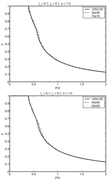
For the second example, we consider an isotropic field. Figure 2 shows com-parison of the fractional flow for caselx = 0.1,lz = 0.1, andσ = 1.0. Both plots in this figure show a good agreement between the fine model and coarse model, regardless of the coarse model dimensions. In conclusion, we would like to note that our coarse scale model tends to perform better for smaller correlation length. In particular, for the upscaling of high correlation length cases, we need larger coarse scale models. This difficulty can be relieved by introducing the nonuniform coarsening, which is a subject of further research.
0 0.5 1 1.5 2 0
0.1 0.2 0.3 0.4 0.5 0.6 0.7 0.8 0.9 1
F
PVI
120x120 30x30 10x10 l
x = 0.40, lz = 0.04, σ = 1.5
0 0.5 1 1.5 2
0 0.1 0.2 0.3 0.4 0.5 0.6 0.7 0.8 0.9 1
PVI
F
120x120 40x40 20x20 l
x = 0.40, lz = 0.04, σ = 1.5
Figure 1 – Comparison of fractional flow of displaced fluid at the production edge for the caselx=0.4,lz=0.04, andσ =1.5 with exponential variogram, andµo/µw=5.
Plots on the top are coarse model with 10×10 and 30×30 elements; plots on the bottom are coarse model with 20×20 and 40×40 elements.
20×20 elements. In the subsequent figures, the following description is used: the upper plot showsS =0.10, the middle plot showsS =0.30, and the lower plot showsS=0.50.
0 0.5 1 1.5 2 0
0.1 0.2 0.3 0.4 0.5 0.6 0.7 0.8 0.9 1
PVI
F
l
x = 0.1, lz = 0.1, σ = 1.0
120x120 30x30 10x10
0 0.5 1 1.5 2
0 0.1 0.2 0.3 0.4 0.5 0.6 0.7 0.8 0.9 1
PVI
F
l
x = 0.1, lz = 0.1, σ = 1.0
120x120 40x40 20x20
Figure 2 – Comparison of fractional flow of displaced fluid at the production edge for the caselx =0.1,lz =0.1, andσ =1.0 with spherical variogram, andµo/µw =5.
Plots on the top are coarse model with 10×10 and 30×30 elements; plots on the bottom are coarse model with 20×20 and 40×40 elements.
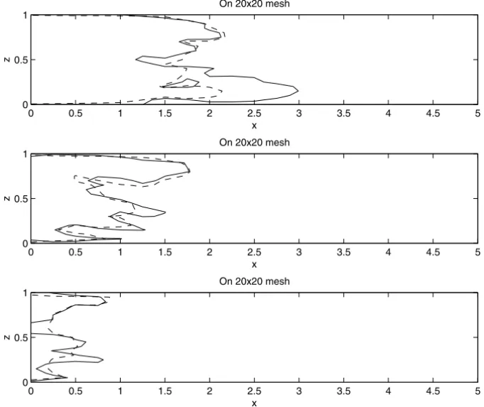
model can follow the fingering indicated by the fine model as seen in lower plot. Similar behavior is shown in Figure 4 for isotropic field withlx =0.1,lz =0.1, andσ = 1. These comparisons also show that the coarse model predicts the contour of saturation better for lower correlation lengths compared to the case with higher correlation length along the main flow direction,lx =0.4,lz =0.04, andσ =1.5.
0 0.5 1 1.5 2 2.5 3 3.5 4 4.5 5 0
0.5 1
x
z
On 20x20 mesh
0 0.5 1 1.5 2 2.5 3 3.5 4 4.5 5
0 0.5 1
x
z
On 20x20 mesh
0 0.5 1 1.5 2 2.5 3 3.5 4 4.5 5
0 0.5 1
x
z
On 20x20 mesh
Figure 3 – Comparison of saturation contours at PVI = 0.15 for the caselx = 0.4,
lz = 0.04, and σ = 1.5 with exponential variogram, and µo/µw = 5. The solid
lines represent the fine grid saturation after averaging onto the coarse grid, while the dashed lines represent the coarse model with 20×20 elements. Upper plots are the
contour ofS =0.10, middle plots are the contour ofS=0.30, and lower plots are the contour ofS=0.50.
this transport coarse model with the primitive model, cf. (2.12). As opposed to the coarse model with macro-diffusion, by its nature, the primitive model does not account for the subgrid effects on the coarse grid. The macro-diffusion is computed using the approximation of the fine scale velocity field by sampling the base functions.
0 0.5 1 1.5 2 2.5 3 3.5 4 4.5 5 0
0.5 1
x
z
On 20x20 mesh
0 0.5 1 1.5 2 2.5 3 3.5 4 4.5 5
0 0.5 1
x
z
On 20x20 mesh
0 0.5 1 1.5 2 2.5 3 3.5 4 4.5 5
0 0.5 1
x
z
On 20x20 mesh
Figure 4 – Comparison of saturation contours at PVI = 0.15 for the caselx = 0.1,
lz = 0.1, and σ = 1.0 with spherical variogram, andµo/µw = 5. The solid lines
represent the fine grid saturation after averaging onto the coarse grid, while the dashed lines represent the coarse model with 20×20 elements. Upper plots are the contour of
S=0.10, middle plots are the contour ofS=0.30, and lower plots are the contour of
S=0.50.
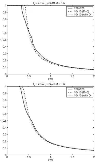
as a reference solution. The dashed line represents the primitive coarse model (D=0), while the dotted line represents the coarse model with macro-diffusion (with D). All coarse models are run on the 10×10 elements.
0 0.5 1 1.5 2 0
0.1 0.2 0.3 0.4 0.5 0.6 0.7 0.8 0.9 1
PVI
F
lx = 0.10, lz = 0.10, σ = 1.5
120x120 10x10 (D=0) 10x10 (with D)
0 0.5 1 1.5 2
0 0.1 0.2 0.3 0.4 0.5 0.6 0.7 0.8 0.9 1
PVI
F
l
x = 0.40, lz = 0.04, σ = 1.5
120x120 10x10 (D=0) 10x10 (with D)
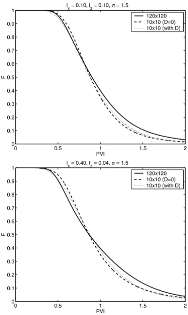
Figure 5 – Comparison of fractional flow of displaced fluid at the production edge. The flux function used is linear,f (S)=S. All coarse models are run on 10×10 elements. Plot on the top corresponds tolx=0.1,lz=0.1, andσ =1.5 with spherical variogram.
Plot on the bottom corresponds tolx = 0.40,lz = 0.04, andσ =1.5 with spherical
variogram.
The performance of the coarse model with macro-diffusion in the case of nonlinear flux function is shown in Figure 6. Here we have used
f (S)= 5S
2
5S2+(1−S)2 and λ(S)=1.
Again, the plot on the top corresponds to isotropic permeability field with
lx = 0.1, lz = 0.1, and σ = 1.5, and the plot on the bottom corresponds to permeability field withlx = 0.40,lz = 0.04, andσ = 1.5. The significance of the diffusion model in these two plots are obvious, in that the macro-diffusion model circumvents the primitive model in predicting the production on and shortly after the breakthrough. Also in this nonlinear flux function case, the model does not seem to be sensitive to the prescribed correlation structures.
To summarize, these computations reveal that the macro-diffusion resulting from the heterogeneity in the flow affects the coarse grid model, which may not be easily disregarded. Moreover, although solely based on the first order approximation, our proposed macro-diffusion model gives a reasonably well performance compared to the widely used primitive model.
Finally, we note that the viscous coupling is not taken into account in the macrodispersion model. In [2, 21] the authors investigated the viscous coupling and their findings indicate that the distinct dispersive regimes can occur depend-ing on the relative strength of nonlinearity and heterogeneity. In particular, the viscosity ratio plays an important role in the stability of the fingering [2]. In the future we plan to use these results for developing new upscaling techniques for two-phase flow. For these approaches the upscaled mobility functions,λ∗(S), that is different fromλ(S), will be employed. More general mobility functions,
λ∗(S,∇S), that depends on bothS and∇S, will be also considered. We have employed the latter in a different upscaling framework in one of our previous works [14].
0 0.5 1 1.5 2 0
0.1 0.2 0.3 0.4 0.5 0.6 0.7 0.8 0.9 1
PVI
F
l
x = 0.10, lz = 0.10, σ = 1.5
120x120 10x10 (D=0) 10x10 (with D)
0 0.5 1 1.5 2
0 0.1 0.2 0.3 0.4 0.5 0.6 0.7 0.8 0.9 1
PVI
F
l
x = 0.40, lz = 0.04, σ = 1.5
120x120 10x10 (D=0) 10x10 (with D)
Figure 6 – Comparison of fractional flow of displaced fluid at the production edge. The flux function used is nonlinear,f (S)= 5S2
5S2+(1−S)2. All coarse models are run on 10×10
elements. Plot on the top corresponds tolx=0.1,lz=0.1, andσ =1.5 with spherical
variogram. Plot on the bottom corresponds tolx =0.40,lz =0.04, andσ =1.5 with spherical variogram.
the atmospheric level. The typical Richards’ equation that we consider here is the so-called mixed formulation, in which the mass storage and transport are expressed in terms of water content and pressure head, respectively:
∂θ (p)
∂t − ∇ ·(kkrw(p)∇p)−
∂ (kzkrw(p))
∂z =0, (3.18)
Fine Model, 256×256 Coarse Model, 32×32
0 0.2 0.4 0.6 0.8 1 0 0.2 0.4 0.6 0.8 1
Figure 7 – Two-scale approximation of the Richards’ equation. Comparison of water pressure between the fine model (left) and the coarse model (right).
The two-scale finite volume method described in Section 2 is applied to (3.18), where the resulting coarse model employs the same base functions as the linear problem. This approximation is motivated by the homogenization results of this class of equation [27, 28]. The analysis and more detailed description of this application will appear elsewhere.
of Richards’ equation is handled using the Picard iteration first proposed in [4]. The figure shows comparison of the water pressure plotted on 257×257 grids obtained using the fine model (left) and the coarse model (right). The fine model uses 256×256 elements, while the coarse model uses 32×32 elements. It is apparent from the figure that the coarse model agrees with the fine model.
4 Summary
In this paper we considered subgrid models for porous media flows. Upscal-ing procedures have been proposed for some multiphase flow applications and numerical results are presented. The numerical calculation of pressure and trans-port equations is accomplished in a consistent manner, providing a unified coarse scale model. The model was applied to a number of example cases involving heterogeneous permeability fields, varying linear and nonlinear fine scale flux functions. In essentially all cases considered, the subgrid model performed well on relatively coarse grids.
Acknowledgement
This work was partially supported by the NSF Grant EIA-0218229.
REFERENCES
[1] T. Arbogast and S.L. Bryant, Numerical subgrid upscaling for waterflood simulations. TICAM Report 01–23, http://www.ticam.utexas.edu/reports/2001/index.html.
[2] V. Artus and B. Noetinger, Macrodispersion approach for upscaling two-phase, immiscible flows in heterogeneous porous media. Presented at the 8th European Conference for the Mathematics of Oil Recovery, Freiberg, Germany, September (2002).
[3] J.W. Barker and S. Thibeau, A critical review of the use of pseudo-relative permeabilities for upscaling.SPE Res. Eng.12(1997), 138–143.
[4] M.A. Celia, E.T. Bouloutas and R.L. Zarba, A general mass-conservative numerical solution for the unsaturated flow equation.Water Resour. Res., (1990), pages 1483–1496.
[5] Z. Chen, R.E. Ewing and Z. Shi (editors),Numerical treatment of multiphase flows in porous media, volume 552 ofLecture Notes in Physics, Berlin, (2000). Springer-Verlag.
[6] M.A. Christie, Upscaling for reservoir simulation.J. Pet. Tech., (1996), pages 1004–1010. [7] N.H. Darman, G.E. Pickup and K.S. Sorbie, A comparison of two-phase dynamic upscaling
[8] C.V. Deutsch and A.G. Journel,GSLIB: Geostatistical software library and user’s guide, 2nd edition.Oxford University Press, New York, (1998).
[9] L.J. Durlofsky, Numerical calculation of equivalent grid block permeability tensors for het-erogeneous porous media.Water Resour. Res.,27(1991), 699–708.
[10] L.J. Durlofsky, Coarse scale models of two phase flow in heterogeneous reservoirs: Volume averaged equations and their relationship to the existing upscaling techniques.Computational Geosciences,2(1998), 73–92.
[11] L.J. Durlofsky, R.A. Behrens, R.C. Jones and A. Bernath, Scale up of heterogeneous three dimensional reservoir descriptions.SPE paper 30709, (1996).
[12] L.J. Durlofsky, R.C. Jones and W.J. Milliken, A nonuniform coarsening approach for the scale up of displacement processes in heterogeneous media. Advances in Water Resources, 20(1997), 335–347.
[13] W.E. and B. Engquist, The heterogeneous multi-scale methods. Comm. Math. Sci.,1(1) (2003).
[14] Y. Efendiev and L. Durlofsky, Accurate subgrid models for two phase flow in heteroge-neous reservoirs. Paper SPE 79680 presented at the SPE Reservoir Simulation Symposium, Houston, June 3–5, (2003).
[15]Y.R. Efendiev, Exact upscaling of transport in porous media and its applications. IMA Preprint Series, 1724, October, 2000, http://www.ima.umn.edu/preprints/oct2000/oct2000.html.
[16] Y.R. Efendiev and L.J. Durlofsky, Numerical modeling of subgrid heterogeneity in two phase flow simulations.Water Resour. Res.,38(8) (2002).
[17] Y.R. Efendiev, L.J. Durlofsky and S.H. Lee, Modeling of subgrid effects in coarse scale sim-ulations of transport in heterogeneous porous media.Water Resour. Res.,36(2000), 2031– 2041.
[18] Y.R. Efendiev, T.Y. Hou and X.H. Wu, Convergence of a nonconforming multiscale finite element method.SIAM J. Num. Anal.,37(2000), 888–910.
[19] R.E. Ewing, Mathematical modeling and large-scale computing in energy and environmental research. In:The merging of disciplines: new directions in pure, applied and computational mathematics (Laramie, Wyo., 1985), pages 45–59. Springer, New York, (1986).
[20] R.E. Ewing, Upscaling of biological processes and multiphase flow in porous media. In:
Fluid flow and transport in porous media: mathematical and numerical treatment (South Hadley, MA, 2001), volume 295 ofContemp. Math., pages 195–215. Amer. Math. Soc., Providence, RI, (2002).
[21] F. Furtado and F. Pereira, Crossover from nonlinearity controlled to heterogeneity controlled mixing in two-phase porous media flows.Computational Geosciences,7(2003), 115–135. [22] V. Ginting, Analysis of a two-scale finite volume element for elliptic problem. Preprint, to
[23] T.Y. Hou and X.H. Wu, A multiscale finite element method for elliptic method for elliptic problems in composite materials and porous media. Journal of Computational Physics, 134(1997), 169–189.
[24] T.Y. Hou, X.H. Wu and Z. Cai, Convergence of a multiscale finite element method for elliptic problems with rapidly oscillating coefficients.Math. Comp.,68(227) (1999), 913–943. [25] P. Jenny, S.H. Lee and H.A. Tchelepi, Multi-scale finite-volume method for elliptic problems
in sub-surface flow simulation.Journal of Computational Physics,187(2003), 47–67. [26] P. Langlo and M.S. Espedal, Macrodispersion for two-phase, immisible flow in porous media.
Advances in Water Resources,17(1994), 297–316.
[27] A.K. Nandakumaran and M. Rajesh, Homogenization of a nonlinear degenerate parabolic differential equation.Electron. J. Differential Equations,17(2001), 1–19 (electronic). [28] A. Pankov, G-convergence and homogenization of nonlinear partial differential operators.
Kluwer Academic Publishers, Dordrecht, (1997).
[29] L.A. Richards, Capillary conduction of liquids through porous mediums.Physics,1(1931), 318–333.
[30] H. Wackernagle,Multivariate geostatistics: an introduction with applications. Springer, New York, (1998).
[31] T.C. Wallstrom, M.A. Christie, L.J. Durlofsky and D.H. Sharp, Effective flux boundary condi-tions for upscalling porous media equacondi-tions.Transport in Porous Media,46(2002), 139–153. [32] T.C. Wallstrom, S. Hou, M. Christie, L.J. Durlofsky, D.H. Sharp and Q. Zou, Application of effective flux boundary conditions to two-phase upscaling in porous media.Transport in Porous Media,46(2002), 155–178.
[33] W. Zijl and A. Trykozko, Numerical homogenization of two-phase flow in porous media.