Copyright © 2004 SBMAC www.scielo.br/cam
On stochastic modeling of groundwater flow
and solute transport in multi-scale
heterogeneous formations
BILL X. HU1,2, JICHUN WU1,3 and CHANGMING HE1,2
1Florida State University, Department of Geological Sciences, Tallahassee, FL 32306, USA 2Hydrology Program, University of Nevada, Reno, USA
3Department of Earth Sciences, Nanjing University, China
E-mail: [email protected] / [email protected] / [email protected]
Abstract. A numerical moment method (NMM) is applied to study groundwater flow and solute
transport in a multiple-scale heterogeneous formation. The formation is composed of various materials and conductivity distribution within each material is heterogeneous. The distribution of materials in the study domain is characterized by an indicator function and the conductivity field
within each material is assumed to be statistically stationary. Based on this assumption, a general expression is derived for the covariance function of the composite field in terms of the covariance of the indicator variables and the statistical properties of the composite materials. The NMM is used to investigate the effects of various uncertain parameters on flow and transport predictions in two case studies. It is shown from the study results that the two-scale stochastic processes of heterogeneity will both significantly influence the flow and transport predictions, especially for
the variances of hydraulic head and solute fluxes. This study also shows that the NMM can be used to study flow and transport in complex subsurface environments. Therefore, the method may be applicable to complex environmental projects.
Mathematical subject classification: 60H30, 60G60.
Key words: heterogeneity, multi-scale, groundwater flow, solute transport.
1 Introduction
It is a well known that at a field scale, geological formations are heterogeneous, and the groundwater flow and solute transport processes in the formation are
considerably affected by the heterogeneity of the formation properties. In the last two decades, many stochastic theories have been developed for groundwater flow and solute transport in heterogeneous porous media [e.g., Dagan, 1989; Gelhar, 1993; Cushman, 1997; Zhang, 2002]. In development of the theories, it is common to assume that the spatial distributions of the medium properties can be characterized by one single correlation scale. This assumption was based on some field studies [Hoeksema and Kitanitis, 1984; Gelhar, 1993], as well as on the notion of the existence of a discrete hierarchy of scales of heterogeneity [Dagan, 1986], with disparity between the scales such that when modeling groundwater flow and solute transport at one scale, variations at other scales can either be averaged out (if other scales are much smaller), or be modeled as a deterministic trend (if other scales are much larger). However, hydraulic properties of many natural media exhibit heterogeneity at multi-scales [Wheatcraft and Tyler, 1998], where the heterogeneity at any scale cannot be averaged out, nor be treated as a deterministic trend.
The usual approach to dealing with multi-scale heterogeneity is simply to increase the variance of stationary processes and not account for the structure of the heterogeneity. This simplification leads to the increase of the variances of hydraulic parameters like conductivity and make the stochastic solution invalid since stochastic groundwater flow models usually rely on smallσf2, the variance of log transformed conductivity.
boundaries of the large-scale features cannot be very well defined due to incom-plete knowledge about them, they also need to be treated as random variables. This kind of media are called multi-(or dual-) scale heterogeneous media. This study focuses on the influence of the multi-scale heterogeneity on groundwater flow and solute transport processes.
A medium with multi-scale heterogeneity is generally nonstationary (statisti-cally non-omogeneous). Solute transport in a nonstationary permeability field is a relatively new research area. Recently, a theoretical framework for solute flux through spatially nonstationary flows in porous media has been developed [Zhang et al., 2000; Wu et al., 2003]. The solute flux depends on the solute travel time and transverse displacement at a fixed control plane. The solute flux statistics (mean and variance) were derived using a Lagrangian framework and were expressed in terms of the probability density functions (PDFs) of particle travel time and transverse displacement. These PDFs were evaluated through the first two moments of travel time and transverse displacement and the as-sumed distribution function. This approach was applied to study solute transport in multiscale media, where random heterogeneities exist at some small scale while deterministic geological structures and patterns can be prescribed at some larger scale. Lu and Zhang [2002] applied moment equation approach to study groundwater flow in a multimodal heterogeneous medium, where the large-scale heterogeneity, the distribution of the various media, is also stationary. In this study, we will firstly extend the flow study to a multi-scale medium, then study solute transport in this medium and also in a multimodal medium.
2 Mean and covariance of a log-hydraulic conductivity field
in a multiple-scale heterogeneous formation
Let us consider a formation composed of k distinct features (e.g., layers, zones, or facies). The process of log hydraulic conductivity, Y (x) of the formation is represented by a k-dimensional stochastic process, Z(x) = (Y1(x), , Yk(x)′,
and the indicator, I (x), is represented by a process I (x) = (I1(x), , Ik(x))′,
where the possible values of I (x) areRk base vectors: e1.e2, , ek, that is each
the definition of the final process Y (x) as a dot product (below), which is the only reason we used it. Further, the probability that I (x) = e1 is p1(x), that
is p(I (x) = e1) = p1(x) for i = 1, . . . , k. The relationship between the two
stochastic processes are assumed to be mutual independent, which means that
I (x) is independent (as a process) from Z(x), and vice versa. The process of
Y (x)is defined as,
Y (x)= k
i=1
Yi(x)Ii(x) (1)
Y (x) is a scalar product. This definition of Y (x) generalizes the processes de-scribed by Rubin [1995] and Zhang [2002], where k = 2.
Under the condition of mutual independence betweenI and Z, we obtain the mean of Y in a two-scale heterogeneous formation as
Y (x) = k
i=1
Yi(x)pi(x) (2)
By definition, the covariance ofY at any two points, x ands, are expressed as
CY(x,s) =
[Y (x)− Y (x)] [Y (x)− Y (x)]
= Y (x)Y (s) − Y (x)Y (x) (3)
Based on (2), Y (x) Y (s)can be derived as
Y (x) Y (x) = k
i=1
Yi(x)pi(x) k
j=1
Yj(x)pj(s)
= k
i,j=1
Yi(x) Yj(s)pi(x)pj(s)
(4)
We define two notations,
pij(x,s) = p(I (x)= ei, I (s) = ej) and
Then, Y (x)Y (s)is derived as,
Y (x)Y (s) = k
i,j=1
Yi(x)Yj(s)| I (x) = ei, I (s)= ejpij(x,s)
= i=j
Yi(x)Yj(s)pij(x,s)+ k
i=1
Yi(x)Yi(s)pii(x,s)
(5)
In the derivation of (5), independence of Y and I is applied. Further, due to the independence ofYi′ and Yj′, whereYl′ = Yl − Yl(l = i, j ), we can obtain
Y (x)Y (s) = i=j
Yi(x)Yj(s)pij(x,s)
+ k
i=1
CY,ii(x,s)+ Yi(x)Yi(s)
pii(x,s)
= k
i,j=1
Yi(x)Yj(s)pij(x,s)+ k
i=1
CY,ii(x,s)pii(x,s)
(6)
From (4) and (6), the expression of CY(x,s)is obtained as
CY(x,s) = k
i,j=1
Yi(x)Yj(s)pij(x,s)−pi(x)pj(s)
+ k
i=1
CY,ii(x,s)pii(x,s)
(7)
Equation (7) is the general expression ofCY(x,s)without any assumption on the
structure of the process I. For a specific field site, we need to obtain the joint probability,pij(x,s), from field investigations to calculateCY(x,s).
The correlation structure of the process I can be expressed as CI,ij(x,s) =
pij(x,s)−pi(x)pj(s). Equation (7) can be rewritten as
CY(x,s) = k
i,j=1
Yi(x)Yj(s)CI,ij(x,s)
+ k
i=1
CY,ii(x,s)(CI,ii(x,s)+pi(x)pi(s))
Equation (8) is the expression for the covariance function of the composite field in terms of the covariance of the indicator variables and the properties of the composite materials.
The expressions of conductivity covariance in two-scale heterogeneous media in (7) and (8) are equivalent to those derived by Lu and Zhang [2002] and generalize the previous studies on many specific cases [e.g., Zhang 2002]. By setting x = s in (7), or (8), the variance ofY (x)is obtained as
σY2(x) = k
i=1
pi(x)σY2i(x)+
k
i=1
pi(x)Yi(x)2
− k
i,j=1
pi(x)pj(x)Yi(x)Yj(x)
(9)
It is obvious that the distribution ofY (x)can be highly nonstationary even though the distribution of Yi(x) in each subunit is stationary. If the two stochastic
processes of I (x)andYi(x)are both stationary, thenσY2 will be a constant.
3 The statistics of hydraulic conductivity in special cases
The general expression of the velocity covariance in a two-scale heterogeneous medium is very complicated. The expression can be greatly simplified in some specific cases. Here we will use couple of examples to show to how to sim-plify the results according to the specific field conditions. A few studies have been conducted to study a natural medium with bimodal distribution of hy-draulic conductivity [e.g., Desbarats, 1987, 1991; Rubin and Journel, 1991; Russo et al., 2001]. The bimodal distribution is a special case of this study. Let
k = 2 in (8), we obtain the covariance of log-hydraulic conductivity in a bimodal heterogeneous medium as,
CY(x.s) = Y1(x)Y1(s)CI,11(x,s)+ Y2(x)Y1(s)CI,22(x,s) + Y1(x)Y2(s)CI,12(x,s)+ Y2(x)Y1(s)CI,21(x,s) +CY,11(x,s)(CI,11(x,s)+p1(x)p1(x))
+CY,22(x,s)(CI,22(x,s)+p2(x)p2(s))
Using the relationships (the derivation is shown in Appendix)
CI,11+CI,12 = 0, CI,21 +CI,22 = 0 (11)
(10) can be rewritten as
CY(x,s) = CY,11(x,s)(CI,11(x,s)+p1(x)p1(s)) +CY,22(x,s)(CI,22(x,s)+p2(x)p2(s))
+ Y1(x)Y1(s)CI,11(x,s)+ Y2(x)Y2(s)CI,22(x,s) − Y1(x)Y2(s)CI,11(x,s)− Y2(x)Y1(s)CI,22(x,s)
(12)
By using the relationships in bimodal medium, p2(x) = 1−p1(x)andp2(s) =
1 −p1(s), and assuming CI,11(x,s) = CI,22(x,s) = CI(x,s), then (12) can be
simplified as
CY(x,s) = CY,11(x,s)[CI(x,s)+p1(x)p1(s)]
+CY,22(x,s){CI(x,s)+ [1 −p1(x)][1−p1(s)]} +CI(x,s)[Y1(x) − Y2(x)][Y1(s) − Y2(s)]
(13)
Equation (13) is the same as the result in Zhang [2002].
Setting s = x in (13), we can obtain the variance of Y (x) in the bimodal medium as
σY2(x) = p1(x)σ12(x)+p2(x)σ22(x)+(Y1(x) − Y2(x))2
− Y2(x))2p1(x)p2(x) = p1(x)σ12(x)+ [1−p1(x)]σ22(x) +(Y1(x) − Y2(x))2p1(x)[1−p1(x)]
(14)
If we further assume thatI (x)is also stationary as the case considered by Rubin and Journel [1991], then Eqs. (2), (13) and (14) become
Y = p1Y1 +(1 −p1)Y2 (15)
CY(x,s) = CY(x−s)= CY(r)
= CY,11(r)[CI(r)+p12] +CY,22(r){CI(r)+ [1−p1]2} (16) +CI(r)[Y1 − Y2]2
From (15)-(17), one may notice that Y and σY2 are constant, and CY(x,s) is
stationary. If the difference between the two Y1 and Y2 is large, then the
third terms in (16) and (17) will be dominant for the covariance and variance, respectively. For this reason, Desbarats [1987] treated Y1 andY2 as constants in
a sand-shale formation, only I (x)is assumed to be a stochastic process. In this special case, (16)-(17) can be further simplified as
CY(r) = CI(r)[Y1 − Y2]2 (18)
σY2 = (Y1 − Y2)2p1(1−p1) (19)
Therefore, we conclude that the expression of the conductivity covariance de-veloped in this study generalizes previous study results. The general expression of the covariance in a multi-scale medium may be significantly simplified in special cases.
4 Method of moment for groundwater glow and solute transport
in nonstationary heterogeneous media
In the last two sections, the explicit expressions for the mean, variance and covariance of hydraulic conductivity in a dual-scale medium have been given in terms of the means, variances of the indicator variable and the hydraulic conductivity of the every single material in the medium, which can be obtained through field measurements and geostatistical analysis. The obtained statistics of the hydraulic conductivity will be used as the input data for the calculations of flow and transport.
cal-culation. In this article, the method which is similar to Lu and Zhang’s [2002] work will not be presented, but the calculated results for the head and velocity will be shown in our case studies.
Recently, a numerical method of moment for solute transport in a nonstationary flow field has been developed. Zhang et al. [2000] and Wu et al. [2003] applied a perturbation approach to set up an analytical framework for solute transport in a nonstationary flow field. The method is to predict solute flux in a two-dimensional flow field through a control plane (CP), which is located at some distance downstream from the plume source. The mean solute mass flux component orthogonal to the CP atx,q(t,x), can be expressed as
q(t,x) =
A0
∞
0
ρ0(a)φ (t −τ )f1[τ (x, a)= t, η(x,a)= y]dτ da (20)
where x = (x, y) is the solute predicting point, τ ≡ τ (x;a) is the travel time of the advective particle from point a to the control plane at x, η(x;a) is the transverse location of a streamline passing through the CP, A0 is the source
area,ρ0(a)is the density of the source mass,φ (t )is the source release function.
f1[τ (x, a), η(x,a)]denotes the joint probability density function (PDF) of travel
time t for a particle fromato reachx and the corresponding transverse displace-ment η. The τ and η are random variables and are functions of the underlying random velocity field.
The variance of the solute flux for the point sampling is evaluated as
σq2(t,x) = q2 − q2 (21)
where
q2(t,x) =
A0
A0
ρ0(a)ρ0(b)φ (t −τ1)φ (t −τ2)·f2[τ1(x,a)
= t, η1(x,a) = y, τ2(x,b) = t, η2(x,b) = y]dadb
(22)
Here f2[τ1(x, a), η1(x,a);τ2(x, b), η2(x,b)] is the two-particle joint PDF of
The travel time τ (L;a), the time required for a parcel originated at a to cross the plane x = L, is determined by the Lagrangian velocity, which is related to the Eulerian velocity. The meanτand fluctuation ofτ (L;a),τ′, is expressed, to the first order, as
τ (L;a) = L
ax
dx U1(x,η)
(23)
τ′(L;a) = − L
ax
dx
U12(x,η)[u1(x,η)+g(x,η)η
′] (24)
where
g(x,η) = ∂[U1(x, η)]
∂η |η=η, η
′,
is the fluctuations of η, Ui(x, η) and ui(x, η)(i = 1,2) are the mean and
per-turbation of the Lagrangian velocity, respectively. If the flow field is stationary, thengwill be zero, and (23) and (24) return to the Dagan’s results [Dagan, 1982; 1984]. From (24), we can obtain the covariance of τ (L;a)as
στ1τ2(L, a;L, b)=
L
ax
L
bx
dx1dx2
U12(x1,η1)U22(x2,η2)
u1(x1,η1) u2(x2,η2)
+g(x1,η1)u1(x2,η2)η′1(x1,η1) +g(x2,η2)u1(x1,η1)η′2(x2,η2)
+b1(x1,η1)b1(x2,η2)η′1(x1,η1)η′2(x2,η2)
(25)
The statistical moments ofη, to the first order, are obtained as
dη(x;a)
dx =
U2(x,η)
U1(x,η)
(26)
dη′(x;a)
dx = A(x,η)u1(x,η)+B(x,η)u2(x,η)
where
A(x,η) = −U2(x,η)
U12(x,η),
B(x,η, ξ) = 1
U1(x,η, ξ)
and
C(x,η) = ∂U2(x, η)
∂η |η=η −
U2(x,η)
U1(x,η)
∂U1(x, η)
∂η |η=η.
Multiplying (27) byη′(x2;b), we obtain
dη′(x1;a)η′(x2;b)
dx1
= A(x1,η1)u1(x1,η1)η′(x2;b)
+B(x1,η)u2(x1η)η′(x2;b) +C(x1,η1)η′(x1;a)η′(x2;b)
(28a)
with the initial condition (here we assume the initial positions of parcels are deterministic)
η′(x1;a)η′(x2;b)|x1=0or x2=0 = 0 (28b)
Similarly, we can also obtain the expressions ofu1η′andu2η′. The velocity
correlations, uiuj =, can be obtained from the flow equations and are treated
as known quantities or input data here. Therefore, there are three differential equations for the three unknowns,η′η′ u1η′, and u2η′, so the equations are
solvable. Owing to the complexity of these equations, we solve them numeri-cally.
From (24), the joint momentsτ′(x1;a)η′(x2;b)is obtained as
τ′(x1;a)η′(x2;b) = − x1
ax
dχ
U12(χ ,η)[u1(χ ,η)η
′(x
2;b)
+g(χ ,η, ξ)η′(χ;a)η′(x2;b)]
(29)
method for computing the first moments is similar to the numerical particle tracking method [Hassan et al., 1998]. From (25) and (29), τ′τ′andτ′η′can be obtained based on the calculated results ofη′η′, u1η′and u2η′.
We assume that for each parcel, itsτ andη obey lognormal and normal distri-butions, respectively, their joint PDFs f1[τ (x, a), η(x,a)] for one particle and
f2[τ1(x, a), η1(x,a);τ2(x, b), η2(x,b)]for two particles can be directly related
to the covariances of τ′ and η′. From (20)-(22), one may see that the solute flux is the summation or integral of all parcels’ distributions. Therefore, even if one parcel is assumed to satisfy lognormal and normal distributions in the longitudinal and transverse directions, respectively, the distribution of all plume (the summation of all parcels) in longitudinal and transverse directions could be quite abnormal in some cases due to the variations of the mean movements of the parcels and variances about the means. In the next sections, the methods introduced in this section will be applied to study groundwater flow and solute transport in multi-scale media.
5 Illustrative example: flow and solute transport in a bi-model medium
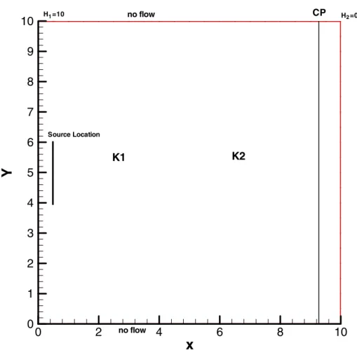
In this section we use a case study to investigate the influences of the two scale stochastic processes of a multi-scale medium on the prediction of groundwater flow and solute transport. The study domain is a square with the size 10×10m2, shown in figure 1. The medium is composed of a lot of small pieces of the two materials, and the two materials are uniformly distributed with each other, like many puzzles, which is so-called bimodal medium. The distributions of two materials are stationary. This phenomenon can be observed in many geological media, such as the lenses of sand, silt and clay inter-bedded with each other in the alluvial sediments, or the various lava mixed together in some igneous rocks. We denoteP (x) = p1(x)to represent the possibility of finding material 1 in the point x. Since the two materials are uniformly distributed,P (x)also represents the percentage of the material 1 in the whole domain. We useλI to represent the
correlation length of the geometry indicatorI (x).
x
Y
0 2 4 6 8 10
0 1 2 3 4 5 6 7 8 9
10 H =10 H =0
Source Location
CP
no flow
no flow
1 2
K1 K2
Figure 1 – Sketch of the study medium.
various calculations for flow and transport. The whole domain is uniformly discretized into 40×40 square elements with a cell size of 0.25×0.25m2. One unit of solute mass is uniformly distributed in the source line.
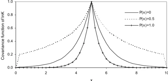
Figure 2 shows the covariance of log-hydraulic conductivity with the reference point at (5.0, 5.0) under P (x) = 0.0,0.5 and 1.0. In this case, we choose
σY21 = 0.4, σY22 = 0.6, λ1 = 0.5m, λ2 = 1.0m and λI = 4.0m. It is shown
from the figure that in comparison with a single material, the mixture of the two materials significantly increases the covariance of the log-hydraulic conductivity in the whole domain, and the conductivity is correlated in a much longer range. Figures 3a and 3b present the distribution of the mean hydraulic head and the variance of the hydraulic head, respectively, along the longitudinal cross-line
x2 = 5.0m with P (x) = 0.0,0.3,0.5,0.7 and 1.0. It is shown from figure
0.0 0.2 0.4 0.6 0.8 1.0
0 2 4 6 8 10
x
Co
v
a
ri
anc
e f
u
n
c
ti
on
of
lnK
P(x)=0 P(x)=0.5 P(x)=1.0
Figure 2 – Covariance function of log hydraulic conductivity for the longitudinal
cross-section with the reference point (5.0,5.0) for various degrees of probability
P (x) =0,0.5 and 1.
comparison with those of one materials. When P (x) = 0.5, which means the compositions of two materials are equal, the predicted variance of hydraulic head reaches its maximum in this case.
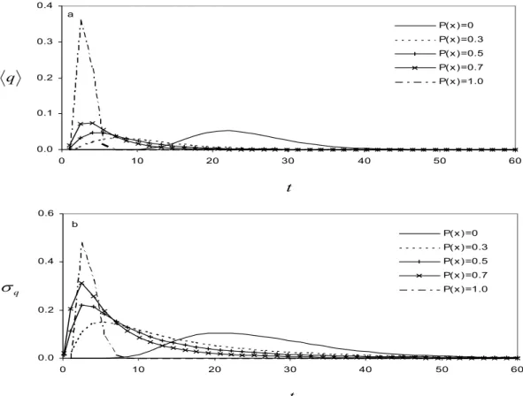
Figures 4a,b show the breakthrough curves of expected values and variances of Q with P (x) = 0.0,0.3,0.5,0.7 and 1.0, respectively. The breakthrough curves of Q change with the variation of P (x), but bounded in the two one-scale cases, P (x) = 0.0 and 1.0. In comparison with the results of one-scale cases, the breakthrough curves in the two-scale cases have longer tails and more dispersion. The σQ curves have the similar shapes to Q’s, butσQ reaches its
maximum whenP (x) = 0.5. Figures 5a,b shows the influences ofP (x)onq at the center point of the control line. The influences are similar to those on Q
and σQ.
a
0 2 4 6 8 10
0 2 4 6 8 10
P(x)=0
P(x)=0.3
P(x)=0.5
P(x)=0.7
P(x)=1.0
H
x
b
0 1 2 3
0 2 4 6 8 10
P(x)=0
P(x)=0.5
P(x)=1.0
P(x)=0.3
P(x)=0.7
h
V
x
Figure 3 – Distribution of (a) the mean hydraulic head, and (b) the standard deviation of
the hydraulic head along the longitudinal cross-sectionx2 = 5.0mfor various degrees
of probabilityP (x)=0,0.3,0.5,0.7 and 1.0.
various materials, the compositions of various materials (which is described by
Pi(x)) and the distribution of the materials, which is described by the
a
0.0 0.2 0.4 0.6 0.8 1.0
0 10 20 30 40 50 60
P(x )=0
P(x )=0.3
P(x )=0.5
P(x )=0.7
P(x )=1.0
Q
t
b
0.0 0.2 0.4 0.6 0.8 1.0
0 10 20 30 40 50 60
P(x )=0
P(x )=0.3
P(x )=0.5
P(x )=0.7
P(x )=1.0 Q
V
t
Figure 4 – Breakthrough curves of the total solute flux through the control plane for
various degrees of probability P (x) = 0,0.3,0.5,0.7 and 1.0, (a) the expected value
Q, (b) the standard deviationσQ.
here we fix its value to be 0.5. In these case studies, we also assume that the log conductivity field in each material and the indicator function I (x) all have exponential auto-covariances. The parameters in the last two columns, i.e., Y
and σY2, are the effective means and variances of the log hydraulic conductivity of the composite medium, which are calculated from Eqs. (2) and (9).
The selection of the eight cases is under the consideration: cases 1, 3 and 5 are used to study the effect of the difference between Y1andY2on flow and
transport processes; cases 3, 7 and 8 are grouped to investigate the effects of the various correlation lengths on flow and transport prediction; the three pairs of case 1 and 2, case 3 and 4, case 5 and case 6 are designed to differentiate the effects of variances on the two scales on prediction of flow and transport. In all these case studies, (external) hydraulic boundary conditions and the locations of the solute source and CP are all same as those shown in figure 1.
a
0.0 0.1 0.2 0.3 0.4
0 10 20 30 40 50 60
P(x )=0 P(x )=0.3
P(x )=0.5
P(x )=0.7
P(x )=1.0
q
t
b
0.0 0.2 0.4 0.6
0 10 20 30 40 50 60
P(x )=0
P(x )=0.3
P(x )=0.5 P(x )=0.7
P(x )=1.0 q
V
t
Figure 5 – Breakthrough curves of the solute flux through the control plane for various
degrees of probabilityP (x) =0.0,0.3,0.5,0.7 and 1.0, (a) the expected valueq, (b)
the standard deviation σq.
Parameter Y1 Y2 σY21 σY22 λ1 λ2 λI Y σY2
Case 1 1.0 -1.0 1.0 1.0 0.5 1.0 4.0 0.0 2.0
Case 2 1.0 -1.0 0.0 0.0 0.5 1.0 4.0 0.0 1.0
Case 3 2.0 -2.0 1.0 1.0 0.5 1.0 4.0 0.0 5.0
Case 4 2.0 -2.0 0.0 0.0 0.5 1.0 4.0 0.0 4.0
Case 5 3.0 -3.0 1.0 1.0 0.5 1.0 4.0 0.0 10.0
Case 6 3.0 -3.0 0.0 0.0 0.5 1.0 4.0 0.0 9.0
Case 7 2.0 -2.0 1.0 1.0 2.0 2.0 4.0 0.0 5.0
Case 8 2.0 -2.0 1.0 1.0 2.0 2.0 2.0 0.0 5.0
Case 9 0.5 -0.5 0.4 0.2 0.5 0.5 1.5 0.0 0.55
Case 10 1.0 -1.0 0.4 0.2 0.5 0.5 1.5 0.0 1.3
0 5 10 15 20 25
0 2 4 6 8 10
case 1 case 2 case 3 case 4 case 5 case 6
h
V
x
Figure 6 – Distribution of (a) the mean hydraulic head, and (b) the standard deviation
of the hydraulic head along the longitudinal cross-sectionx2 =5.0matP (x) =0.5 for
cases 1, 2, 3, 4, 5 and 6, respectively.
Y1-Y2, and small-scale heterogeneity,σY21andσY22, on hydraulic head variance
and solute flux. Figures 6 shows the distribution of σh2 along the longitudinal cross-line x2 = 5.0m for the six cases. Figures 7a,b shows the breakthrough
curves of expected values and variances of total solute flux Q through CP in the six cases. Figures 8a,b present the breakthrough curves of q and σ12, respectively. It is shown from figures 6-8 that the variations of σY2
1 and σ
2 Y2
hardly affectσh2 and Q, but influence σQ, qand σq2. However the influences
are secondary to those caused by Y1-Y2. In these cases, the total variance,
σY2, significantly influence the distribution of head variance, mean and variance of solute flux, and σY2 is largely contributed from the large-scale heterogeneity.
In the above study, the effects ofY1-Y2,σY21,σY22andσY2on flow and transport
have been studies. Here, we would like to group cases 3, 7 and 8 to analyze the effects ?1, ?2and ?I on the flow and transport. Figures 9 shows the distribution of
σh2along the longitudinal cross-linex2 = 5.0mfor the three cases. In comparison
0.00 0.05 0.10 0.15 0.20 0.25 0.30 0.35 0.40
0 5 10 15 20 25 30 35 40 45 50
case 1 case 2 case 3 case 4 case 5 case 6
Q
t
0.0 0.2 0.4 0.6 0.8 1.0 1.2
0 5 10 15 20 25 30 35 40 45 50
case 1 case 2 case 3 case 4 case 5 case 6
Q
V
t
Figure 7 – Breakthrough curves of the total solute flux through the control plane at
P (x) =0.5 for cases 1, 2, 3, 4, 5 and 6, respectively, (a) the expected valueQ, (b) the
0.00 0.01 0.02 0.03 0.04 0.05 0.06
0 5 10 15 20 25 30 35 40 45 50
case 1 case 2 case 3 case 4 case 5 case 6
q
t
0.00 0.05 0.10 0.15 0.20 0.25 0.30 0.35
0 5 10 15 20 25 30 35 40 45 50
case 1 case 2 case 3 case 4 case 5 case 6
q V
t
Figure 8 – Breakthrough curves of the total solute flux through the control plane at
P (x) =0.5 for cases 1, 2, 3, 4, 5 and 6, respectively, (a) the expected valueq, (b) the
0 2 4 6 8 10 12 14
0 1 2 3 4 5 6 7 8 9 10
case 3
case 7
case 8
h V
x
Figure 9 – Distribution of the standard deviation of the hydraulic head along the
longi-tudinal cross-sectionx2 =5.0matP (x)= 0.5 for cases 3, 7 and 8, respectively.
Similarly, from the results of case 7 and 8, one case see thatσh2 increase with the increase of λI.
Figures 10a,b shows the breakthrough curves of expected values and variances of total solute fluxQthrough CP for the three cases. It is shown from the figures that with the increases of ?1, ?2 and λI, Qcurve has an earlier breakthrough
and the high peak, but the tail does not change. The increases of ?1, ?2 and ?I
also lead to the increase of σQ2. Figures 11a,b present the breakthrough curves of q and σq2, respectively. q and σq2 curves are quite different from their counterparts of Qand σQ2, which is caused by the transverse dispersion.
6 Comparison of NMM and Monte Carlo simulation results
0.00 0.05 0.10 0.15 0.20 0.25 0.30
0 5 10 15 20 25 30 35 40 45 50
case 3 case 7 case 8
Q
0.0 0.1 0.2 0.3 0.4 0.5 0.6 0.7 0.8 0.9 1.0
0 5 10 15 20 25 30 35 40 45 50
case 3 case 7 case 8
Q
V
Figure 10 – Breakthrough curves of the total solute flux through the control plane at
P (x) = 0.5 for cases 3, 7 and 8, respectively, (a) the expected value Q, (b) the
0.000 0.005 0.010 0.015 0.020 0.025 0.030 0.035 0.040
0 5 10 15 20 25 30 35 40 45 50
case 3
case 7 case 8
q
0.00 0.05 0.10 0.15 0.20 0.25 0.30 0.35
0 5 10 15 20 25 30 35 40 45 50
case 3 case 7 case 8
q
V
t
Figure 11 – Breakthrough curves of the total solute flux through the control plane at
P (x) =0.5 for cases 3, 7 and 8, respectively, (a) the expected valueq, (b) the standard
the calculation results. In this section, a Monte Carlo numerical simulation method is applied to check the results obtained by the NMM. This kind of study has been conducted for flow in multi-scale media [Winter et al., 2002; Lu and Zhang, 2002]. In this study, we only compare the transport results in a bimodal medium.
6.1 Generation of multi-realizations of hydraulic conductivity field
The study domain is the same as the one shown in figure 1. The study domain is discretized into 100× 100 square elements with a size of 0.1 ×0.1λ2. Two cases, cases 9 and 10 in table 1, are chosen in this section. The assumptions for the bi-model conductivity field made here are the same as those made in section 2. A three-step method is used to generate the bi-model conductivity field. First, according to the conductivity parameters provided in table 1 for Y1
and Y2, 3,000 realizations of the conductivity field are generated for each of the
two media with a Fast Fourier Transform method. Secondly, a Gaussian random field generatorsisimfrom GSLIB [Deutsch, C. V., A. G. Journel, 1998] is applied to generate 3,000 realizations of the geometry indicator field with λI = 1.5 λ
andp1 = p2 = 0.5. Third, each indicator field is combined with one realization
of Y1 and Y2 to form one realization of the bi-modal conductivity field. As an
example, one conductivity realization for case 9 is shown in figure 12.
Figures 13a,b show the histograms of the log hydraulic conductivity realiza-tions for cases 9 and 10. It is shown from the two figures that the bi-model distribution appears only when the difference between Y1 and Y2 is large
enough in comparison withσY21 and/or σY22.
6.2 Groundwater flow and solute transport simulations
The hydraulic boundary conditions are the same as those shown in figure 1, except
H1 = 1.0. The locations of source line and CP are the same as those shown in
Figure 12 – One realization of bimodal conductivity field.
to simulate the movement of solute by a large number of particles. Therefore, the calculation of solute flux across the CP becomes the calculation of arrival times of individual particles reaching the CP. The obtained multi-realizations of the solute flux curve are averaged over realizations to obtain the mean and variance of the solute flux.
Figures 14 and 15 show the results of the Monte Carlo simulation and NMM for two cases. Since the local dispersivity is not considered in the Monte Carlo simulation, the breakthrough curve is not smooth. For case 9, the calculation results of the two methods are almost identical. With the increase of the difference between Y1 and Y2, the NMM results will deviate from those of the Monte
Histogram
0 100 200 300 400
-1,87-1,60-1,34-1,07-0,80-0,54-0,27-0,01 0,26 0,52 0,79 1,06 1,32 1,59 1,85 2,12 2,39
ln(K)
F
requency
(a)
Histogram
0 50 100 150 200 250 300
-2,40 -2,04 -1,67 -1,31 -0,94 -0,58 -0,21 0,15 0,51 0,88 1,24 1,61 1,97 2,34 2,70
ln(K)
F
requency
(b)
This issue needs to be addressed in future study. Generally speaking, NMM captures the dominate characteristics of the breakthrough curves as shown in Figure 14 for case 9, and Figure 15 for case 10.
0 0.01 0.02 0.03 0.04
0 50 100 150 200 250 t(day)
<Q>
NMM MC
0 0.001 0.002 0.003 0.004
0 50 100 150 200 250
t(day)
NMM MC
2 Q ı
Figure 14 – Comparison of calculation results between Monte Carlo simulation and
NMM method for case 9.
7 Summary and conclusions
0 0.01 0.02 0.03 0.04
0 50 100 150 200 250
t(day)
<Q>
NMM MT
0 0.001 0.002 0.003
0 50 100 150 200 250
t(day)
NMM MC
2 Q ı
Figure 15 – Comparison of calculation results between Monte Carlo simulation and
NMM method for case 10.
but dramatically changes the head variance, mean and variance of solute flux. Based on this study, we propose 8 cases to study effects of other uncertainty parameters, which include the small-scale parameters, such as the variances and correlation lengths of log conductivity of the two materials, and large-scale pa-rameters, such as the differences of mean log conductivity values of the two materials and the correlation length of the indicator function. The large-scale and small-scale heterogeneities will both significantly influence the flow and solute transport processes.
The NMM results are compared with those of the Monte Carlo simulation for the bi-model medium. The calculation results of the two methods are consistent with each other for small total variance of log-conductivity (less than 1.3 accord-ing to case 10), but will derivate with each other with the increase of the total variance.
8 Acknowledgments
This work was partially funded by DOE Yucca Mountain Project under contract between DOE and the University and Community College System of Nevada and Teaching and Research Award Program for Outstanding Young Teacher (TRAPOYT) of MOE, China.
9 Appendix
Fork = 2,p2(x)= 1−p1(x). Then we have
p11(x,s) = CI,11(x,s)+p1(x)p1(s) (A1)
p12(x,s) = CI,12(x,s)+p1(x)p2(s)
= CI,12(x,s)+p1(x)−p1(x)p1(s) (A2)
p21(x,s) = CI,21(x,s)+p2(x)p1(s)
= CI,21(x,s)+p1(s)−p1(x)p1(s) (A3)
p22(x,s) = CI,22(x,s)+p2(x)p2(s)
= CI,22(x,s)+1−p1(x)−p1(s)+p1(x)p1(s) (A4)
Since p11(x,s)+ p12(x,s) = p1(x) and p22(x,s)+ p21(x,s) = 1 −p1(x).
REFERENCES
[1] Care S.F. and Fogg G.E., Modeling spatial variabiliyy with one- and multi-dimensional continuous Markov chains, Math. Geology29(7) (1997), 891–918.
[2] Cushman J.H., The Physics of Fluids in Hierarchical Porous Media: Angstroms to Miles, Kluwer Academic, 1997.
[3] Cushman J.H, On measurement, scale, and scaling, Water Resour. Res. 22 (2) (1986), 129–134.
[4] Dagan G., Stochastic theory of groundwater flow and transport: Pore to laboratory, laboratory to formation, and formation to regional scale, Water Resour. Res. 22(9) (1986), 120S–134S.
[5] Dagan G., Flow and Transport in Porous Formations, Springer-Verlag, New York, 1989.
[6] Dagan G., Stochastic modeling of groundwater flow by unconditional and conditional prob-abilities, 2, The solute transport, Water Resour. Res. 18(4) (1982), 835–848.
[7] Dagan G., Solute transport in heterogeneous porous formations, J. Fluid Mech. 145(1984), 151–177.
[8] Desbarats A.J., Numerical estimation of effective permeability in sand-shale formations, Water Resour. Res. 23(2) (1987), 273–286.
[9] Desbarats A.J., Macrodispersion in sand-shale sequence, Water Resour. Res. 26(1) (1991), 153–163.
[10] Deutsch C.V and Journel A.G, GSLIB: Geostatistical Software Library and User’s Guide, 2nd ed. Oxford University Press, New York, 369 pp, 1998.
[11] Gelhar L.W., Stochastic Subsurface Hydrology, Prentice-Hall, Englewood Cliffs, NJ, 1993.
[12] Hassan A.E., Cushman J.H. and Delleur J.W., A Monte Carlo assessment of Eulerian flow and transport peturbation models. Water Resour. Res. 34(5) (1998), 1143–1163.
[13] Hoeksema R.J. and Kitanidis P.K., An application of the geostatistical approach to the inverse problem in two-dimensional groundwater modeling, Water Resour. Res.20(7) (1984), 1003– 1020.
[14] Lu Z. and Zhang D., On stochastic modeling of flow in multimodal heterogeneous formations. Water Resour. Res. 38(10) (2002), 10.1029/2001WR001026.
[15] RubinY. and Journel A.G., Simulation of non-Gaussian space random functions for modeling transport in groundwater, Water Resour. Res. 27(7) (1991), 1711–1721.
[16] Rubin Y., Flow and transport in bimodal heterogeneous formations, Water Resour. Res. 31(10) (1995), 2461–2468.
[18] Wheatcraft S.W. and Tyler S.W., An explanation of scale-dependent dispersivity in hetero-geneous aquifers using concepts of fractal geometry, Water Resour. Res. 24 (4) (1998), 566–578.
[19] Winter C.L., Tartakovsky D.M. and Guadagnini A., Numerical solutions of moment equations for flow in heterogeneous composite aquifers, Water Resour Res. 38 (5) (2002), 10.1029/ 2001WR000222.
[20] Wu Jichun, Hu B. and Zhang D., Applications of nonstationary stochastic theories to solute transport in multi-scale geological media, Journal of Hydrology,275(3-4) (2003), 208–228.
[21] Zhang D., Stochastic Methods for Flow in Porous Media: Coping with Uncertainties, Academic Press, San Diego, Calif., 2002.
[22] Zhang D., Andricevic R. Sun A.Y., Hu B.X. and He G., Solute flux approach to transport through spatially nonstationary flow in porous media, Water Resour. Res. 36 (8) (2000), 2107–2120.