Generalized Classical and Quantum Dynamics
Within a Nonextensive Approach
A. Lavagno
Dipartimento di Fisica, Politecnico di Torino, I-10129 Torino, Italy,
and Istituto Nazionale di Fisica Nucleare, Sezione di Torino, Italy
Received on 20 December, 2004
On the basis of generalized classical kinetic equations, reproducing the stationary distribution of the Tsallis nonextensive thermostatistics, we formulate two generalized Schr ¨odinger equations which satisfy the basic as-sumptions of the quantum mechanics under an appropriate generalization of the operator properties. Moreover, we study the generalization of the previously introduced dynamic equations in a relativistic regime and we apply our results to the study of the rapidity distribution in the relativistic heavy-ion collisions.
1
Introduction
Let us review some basic assumptions of the nonextensive thermostatistics that will be useful in view of the generalized classical and quantum dynamics we will describe.
Starting point of the Tsallis’ generalization of the Boltzmann-Gibbs statistical mechanics is the introduction of a q-deformed entropy functional defined, in a phase space system, as [1]
Sq =−kB Z
dΩpqlnqp , (1)
wherekBis the Boltzmann constant,p=p(x, v)is the phase space probability distribution,dΩstands for the correspond-ing phase space volume element andlnqx= (x1−q−1)/(1−
q)is, for x > 0, the q-deformed logarithmic function. For the real parameter q → 1, Eq.(1) reduces to the standard Boltzmann-Gibbs entropy functional.
In the equilibrium canonical ensemble, under the con-straints imposed by the probability normalization
Z
dΩp= 1, (2)
and the normalizedq-mean expectation value of the energy [2]
hEiq = R
dΩpqH(x, v) R
dΩpq , (3)
the maximum entropy principle gives the probability distrib-ution [2, 3]
p(x, v) = f(x, v)
Zq
, (4)
where
f(x, v) = [1−(1−q)β(H(x, v)− hHiq)]1/(1−q) (5) and
Zq = Z
dΩf(x, v). (6)
Let us note that, depending from the extremization proce-dure, in Ref.[2] the above factorβis only proportional to the Lagrange multiplier, because of the probability distribution is self-referential, while, in Ref.[3],βis actually the Lagrange multiplier associated to the energy constraint.
By using the definitions in Eqs. (4) and (6) into the rela-tionZ1−q
q =
R
dΩpq[3], the following identity holds [4] Z
dΩf(x, v)≡
Z
dΩfq(x, v), (7) and the normalizedq-mean expectation value for a physical observableA(x, v)can be expressed as
hAiq = R
dΩfqA(x, v)
R
dΩfq ≡ 1
Zq Z
dΩfqA(x, v). (8) Therefore, the probability distribution and theq-mean value of an observable have the same normalization factorZq, as in the extensive statistical mechanics. Such a non-trivial prop-erty does not depend on the equilibrium frame but it comes from the normalization condition and holds at any time (if we require that the transport equation conserves the probability normalization or the number of particles). This observation will play a crucial role in the following discussion.
2
From Fokker-Planck equation to
nonextensive Schr¨odinger equation
The linear Fokker-Planck equation in the velocity space can be written as
∂
∂t[f(t, v)] =− ∂ ∂v
·
J(v)[f(t, v)]−D ∂
∂v[f(t, v)] ¸
Of course, the stationary solution of the above equation depends from the explicit expression of the drift J and the diffusion coefficientD. It is easy to see that ifJ andD de-pend on the deformation parameterqby means the following relation
∂Dq
∂v −
βmv
1−(1−q)βEDq+Jq = 0, (10)
whereE =mv2/2, the stationary solution is the power-law
Tsallis distribution function [1, 5]
fq(v) = [1−(1−q)βE]1/(1−q). (11) On the basis of the above observations and following the stochastic quantization procedure, the “nonextensive” linear Schr¨odinger equation can be written as
i~∂ψ
∂t = ˆHqψ , (12)
whereHˆqis theq-deformed Hamiltonian ˆ
Hq =
ˆ
H
1−(1−q)i
~Htˆ
, (13)
ˆ
H is the Hamiltonian operator and we have assumed that it contains no explicit time dependence. The right side of Eq.(12) must be seen as a power series of the operator (1−q)iHt/ˆ ~forq≈1. Equation (12) does not admit factor-ized solutions but can be integrated to find the wave function at any timetbfrom the state at any other timetaas follows
ψ(tb) = ˆUq(tb, ta)ψ(ta), (14) where ta < tb and we have introduced the generalized q -deformed time evolution operator
ˆ
Uq(tb, ta) =
[1−(1−q)~iHtˆ b]
1/(1−q)
[1−(1−q)i
~Htˆ a]1/(1−q)
≡ expq
³
−~iHtˆ b ´
expq ³
−~iHtˆ a
´. (15)
In the second equivalence we have used the definition of the Tsallisq-deformed exponential
exq = [1 + (1−q)x]1/(1−q), (16) which satisfies the properties: eq(lnqx) = xand eq(x)·
eq(y) =eq[x+y+ (1−q)xy].
Theq-deformed time evolution satisfies thefundamental composition law. In fact, if two time translations are per-formed successively, the corresponding operatorsUˆq are re-lated by
ˆ
Uq(tb, ta) = ˆUq(tb, tc) ˆUq(tc, ta), (17) for anytc∈(ta, tb). It is important to observe that the oper-atorUˆq is not a unitary operator in the common sense, how-ever if we observe that the q-deformed exponential, defined in Eq.(16), satisfies the following properties
exq e−2−xq = 1, (18)
eixq (eix2−q)∗ = 1⇔(eix2−q)∗= (eixq )−1, (19)
it appears natural to define theq-adjointof an operatorOˆqas
ha|Oˆ†q|bi=hb|Oˆ2−q|ai∗. (20)
On the basis of the above prescription, theq-deformed time evolution operator can be view as aq-unitary operator
ˆ
Uq†(tb, ta) = [ ˆUq(tb, ta)]−1, (21)
and
[ ˆUq(tb, ta)]−1= ˆUq(ta, tb). (22)
Moreover, on the basis of the definition (20) we can see that theq-deformed HamiltonianHˆq is aq-hermitian operator, in the sense that
ˆ
Hq†≡Hˆ2∗−q= ˆHq. (23)
Theq-Schr¨odinger equation forUˆqcan be written as
i~∂Uˆq(t, ta)
∂t = HˆqUˆq(t, ta), (24) i~∂Uˆq(t, ta)
−1
∂t = −Uˆq(t, ta)
−1Hˆ
q. (25)
Furthermore, theq-deformed Schr¨odinger equation (12) con-serves the probability. In fact, if we define the probability density of a single particle in a finite volume as
ρq =ψ†qψq≡ψ∗2−qψq, (26)
it is easy to show that
∂ ∂t
Z
d3x ρq = 0. (27)
Finally, we want to stress that the structure of the
Heisemberg’s correspondence principleis invariant in theq -deformed quantum mechanics. In fact, if we define, as usual, the Heisenberg operatorOˆqH(t)as
ˆ
OqH(t) = ˆUq(t, ta)
−1Oˆ
q(t) ˆUq(t, ta), (28)
andOˆq(t)is an arbitrary observable in the Schr¨odinger pic-ture, it is easy to show that
dOˆqH
dt =
i
~[ ˆHqH,OˆqH] + ∂OˆqH
3
From
non-linear
Fokker-Planck
equation to non-linear and
nonex-tensive Schr¨odinger equation
A class of anomalous diffusions are currently described through the non-linear Fokker-Planck equation (NLFPE)
∂
∂t[f(t, x)]
µ=− ∂
∂x ·
J(x)[f(t, x)]µ−D ∂
∂x[f(t, x)]
ν¸ ,
(30) whereDandJare the diffusion and drift coefficients, respec-tively. Tsallis and Bukman [12] have shown that, for linear drift, the time dependence solution of the above equation is a Tsallis-like distribution withq= 1 +µ−ν. The norm of the distribution is conserved for all times only ifµ= 1, therefore we will limit the discussion to the caseν= 2−q.
The main characteristic of anomalous diffusion is that the mean squared displacement is not proportional to timetbut rather to some power oft. If the scaling is faster thant, we say that the system is superdiffusive; if it slower thant, we say that the system is subdiffusive. Often these processes are strictly connected to memory effects and described by non-linear evolution equations.
In this section we want to show that it is possible to intro-duce a different generalization of the Schr¨odinger equation on the basis of the above NLFPE.
Following, as before, the stochastic quantization and, for simplicity, restricting the discussion to the free case, we ob-tain the non-linear Schr¨odinger equation
i~∂ψ
∂t =−
~2 2m
∂2
∂x2ψ
ν.
(31) The above equation appears interesting because, differently from Eq.(12), admits a factorized solution ψ = φ(t)ϕ(x), whereφ(t)obeys to the equation
i~dφ(t)
dt =Eφ(t)
ν,
(32) and the time independent wave functionϕ(x)can be obtained from theν-deformed eigenvalue equation
∂2ϕ(x)ν
∂x2 +k
2ϕ(x) = 0,
(33) wherek=p
2mE/~2. It is easy to see that the solution of
the above equations can be written as
φ(t) =
·
1−(1−ν)iE
~t
¸1/(1−ν)
, (34)
ϕ(x) =
"
1 + p ν−1
2ν(ν+ 1)ikx
#1/(1−ν)
. (35)
Analogously to the previous section, we can introduce the
q-deformed time evolution operator by means of the follow-ing expression
ψ(tb) = ˆUq(tb, ta)ψ(ta), (36)
where ˆ
Uq(tb, ta) = expq µ
−i ~H
tb−ta
ψ(ta)1−ν ¶
= hexpq µ
−i ~H
ta−tb
ψ(tb)1−ν ¶
i−1 . (37)
It is also interesting to note that by using the property (18) of theq-exponential,Uˆq(tb, ta)can be written in a more symmetric form as follows
ˆ
Uq(tb, ta) = "
1−(1−ν)i
~Hˆ
tb−ta
ψ(ta)1−ν
1−(1−ν)~iHˆ
ta−tb
ψ(tb)1−ν
#1/2(1−ν)
. (38)
From the above expressions we can see that the time evo-lution operatorUˆq(tb, ta)depends explicitly from the initial
a and the final state b and not only from the time differ-encetb−ta. Such a behavior is motivated by the non-linear Fokker-Planck equation (30) that implies anomalous diffu-sion and it is related to memory effects [12]. For this reason the composition law is not satisfied, anomalous diffusion and memory effects imply thatUˆq can not be seen as a represen-tation of the abelian group.
Finally, we observe the properties (21) and (22) still hold in the non-linear generalization if we assume, as before, the adjoint operator rule of Eq.(20).
4
Nonextensive relativistic dynamics
In the previous sections we have introduced generalized clas-sical and quantum evolution equation in the framework of Tsallis nonextensive conditions. Because of the growing in-terest to high energy physics applications of nonextensive thermostatistics [6], in this Section we want to study the for-mulation of the relativistic nonextensive kinetic equations. Let us start defining the basic macroscopic variables in the language of relativistic kinetic theory. Because we are go-ing to describe a non-uniform system in the phase space, we introduce the particle four-flow as [7, 8]
Nµ(x) = 1
Zq Z d3p
p0 p
µf(x, p), (39)
and the energy-momentum flow as
Tµν(x) = 1
Zq Z d3p
p0 p
µpνfq(x, p),
(40)
where we have set ~ = c = 1, x ≡ xµ = (t,x), p ≡
pµ = (p0,p)andp0=p
p2+m2is the relativistic energy.
The four-vectorNµ= (n,j)contains the probability density
In order to derive a relativistic Boltzmann equation for a dilute system in nonextensive statistical mechanics, we con-sider the finite volume elements∆3xand∆3pin the phase
space. These volume elements are large enough to contain a very large number of particles but also small enough com-pared to the macroscopic dimension of the system. In the Lorentz frame, the particle fraction∆N(x, p)in the volume ∆3x∆3pcan be written as
∆N(x, p) = N
Zq Z
∆3x Z
∆3p
dΩfq(x, p), (41)
whereNis the total number of particles of the system. With respect to the observer’s frame of reference, the above ex-pression becomes
∆N(x, p) = N
Zq Z
∆3σ Z
∆3p
d3σµd
3p
p0 p
µfq(x, p), (42)
whered3σ
µ is a time-like three-surface element of a plane space-like surfaceσ[9]. Requiring that the net flow through surface ∆3σ of element ∆4xvanishes in absence of
colli-sions, we have: pµ∂
µfq(x, p) = 0. While considering colli-sions between particles, the Boltzmann equation becomes
pµ∂µfq(x, p) =Cq(x, p). (43)
Cq(x, p)is theq-deformed collision term that, under the hy-pothesis that only binary collisions occur in the gas, can be expressed as
Cq(x, p) = 1 2
Z d3p
1
p0 1
d3p′
p′0
d3p′
1
p′0 1
n
hq[f′, f′1]W(p′, p′1|p, p1)
−hq[f, f1]W(p, p1|p′, p′1)
o
. (44)
In the above equation, we have set W(p, p1|p′, p′1)as the
transition rate between two particle state with initial four-momentumpandp′ and a final state with four-momentap
1
andp′
1; hq[f, f1] is the correlation function related to two
particles in the same space-time position but with different four-momenta p andp1, respectively. The factorization of
hq in two single probability distributions (uncorrelated par-ticles at the same spatial point) is the celebrated hypothe-sis of molecular chaos (Boltzmann’s Stosszahlansatz). Thus, the functionhqdefines implicitly a generalized nonextensive molecular chaos hypothesis.
By assuming the conservation of the energy-momentum in the collisions (i.e.pµ+p′µ=pµ
1+p′
µ
1) and requiring that
the correlation functionhq is symmetric and always positive (hq[f, f1] =hq[f1, f],hq[f, f1]>0), it is easy to show that
collision term satisfies the following property
F[ψ] =
Z d3p
p0 ψ(x, p)Cq(x, p) = 0, (45)
if
ψ(x, p) =a(x) +bµ(x)pµ , (46) wherea(x)andb(x)are arbitrary functions.
By choosingψ=const.and using the Boltzmann equa-tion (43), then Eq.(45) implies
∂ ∂t
Z
dΩfq(x, p) = 0, (47) and this is nothing else that the conservation of the probabil-ity normalizationZq. Otherwise, by settingψ = bµpµ, we have from Eq.(45)
∂νTµν(x) = 0, (48) which implies the energy and the momentum conservation.
Let us remark that to have conservation of the probability normalization, energy and momentum, it is crucial that not only the collision termCq be explicitly deformed by means of the functionhq, but also the streaming termpµ∂µfq. This matter of fact is a direct consequence of the nonextensive statistical prescription of the normalizedq-mean expectation value and is not taken into account in the non-relativistic for-mulation of Ref.[10].
The relativistic localH-theorem states that the entropy production σq(x) = ∂µSqµ(x) at any space-time point is never negative.
Assuming the validity of Tsallis entropy (1), it ap-pears natural to introduce the nonextensive four-flow entropy
Sµ
q(x)as follows
Sµq(x) =−kB Z d3p
p0 p
µfq(x, p)[ln
qf(x, p)−1]. (49) On the basis of the above equation the entropy production can be written as
σq(x) =−kB Z d3p
p0 lnqf p
µ∂
µfq ≡ −kBF[lnqf], (50) where the second identity follows from the Boltzmann equa-tion (43) and the definiequa-tion ofF[ψ]in Eq.(45). After simple manipulations, Eq.(50) can be rewritten as
σq(x) =
kB
8
Z d3p 1
p0 1
d3p 1
p0 1
d3p′
p′0
d3p 1′
p′0
1
³
lnqf′+ lnqf′1−
lnqf+ lnqf1
´
×nhq[f′, f′1]W(p′, p′1|p, p1)−
hq[f, f1]W(p, p1|p′, p′1)
o
. (51)
By assuming the detailed-balance property, we have that the entropy production is always an increasing function, if
q >0and if the functionhqsatisfies the general condition
hq[f, f1] =hq[lnqf+ lnqf1], (52)
in addition to be symmetric and always positive.
Because the nonextensive formalism reduces to the stan-dard Boltzmann kinetic formulation for q → 1, it appears natural to postulate the q-generalized Boltzmann molecular chaos hypothesis as
whereeq(x)is the Tsallisq-exponential function introduced in Eq.(16). Let us note that a similar expression for the func-tionhq was previously introduced in Ref.s [10] and a rigor-ous justification of the validity of the ansatz (53) can be found only by means of a microscopic analysis of the dynamics of correlations in nonextensive statistics.
5
Rapidity distribution in relativistic
heavy-ion collisions
In this Section we want to show as nonextensive statistical ef-fects can be very relevant also in the phenomenological inter-pretation of the high-energy nuclear collisions data. In fact, the quark-gluon plasma close to the critical temperature is a strongly interacting system [6]. For such a system, the color-Coulomb coupling parameter of the QGP can be defined, in analogy to the classical plasma, as
Γ≈C g
2
r0T
>1, (54)
whereC= 4/3or 3 is the Casimir invariant for the quarks or gluons, respectively,αs=g2/(4π) = 0.2÷0.5andr0is the
mean particle distancer0≃n1/3≃0.5fm.
Near the phase transition, the interaction range is much larger than Debye screening length (small number of par-tons in Debey sphere). In fact, λD = 1/µ ≤ 0.2 fm, if we use the non-perturbative estimate µ = 6T. The Coulomb radius for a thermal parton with energy3Tis given by< r >= Cg2/3T = 1÷6 fm. Therefore one obtain
< r > /λD = 5÷30. In other words, memory effects and long–range color interactions give rise to the presence of non–Markovian processes in the kinetic equation affecting the thermalization process toward equilibrium as well as the standard equilibrium distribution.
We are going to study the evolution of the rapidity distri-bution from a macroscopic point of view by using the non-linear relativistic Fokker-Planck equation (30) in the space of the rapidity distribution y. We show that the observed broad rapidity shape could be a signal of non-equilibrium properties of the system. Let us note that a similar ap-proach, within a linear Fokker-Planck equation, has been previously studied in Ref.[11] by using a linear drift in the space of the rapidity and a free parameter diffusion coeffi-cient. With this choice, the author found a strongly viola-tion of the fluctuaviola-tion-dissipaviola-tion theorem. We will see that generalizing the Brownian motion to the relativistic kinetic variables, the standard Einstein relation is satisfied and Tsal-lis non-extensive statistics emerges in a natural way from the non-linearity of the Fokker-Planck equation.
Basic assumption of our analysis is that the rapidity distri-butionyis not appreciably influenced by transverse dynamics which is considered in thermal equilibrium. Such hypothesis is well confirmed by the experimental data and adopted in many theoretical works [13, 14, 15]. A crucial rˆole in the so-lution of the above NLFPE plays the choice of the diffusion and the drift coefficients. Such a choice influences the time evolution of the system and its equilibrium distribution.
Since the temperature at freeze-out exceeds 100 MeV, quantum statistical effects are negligible and the Boltzmann approximation is usually adopted, therefore the single parti-cle equilibrium distribution is written as
Ed
3N
d3p ∝Eexp(−E/T)
≡m⊥ cosh(y) exp(−m⊥cosh(y)/T), (55)
whereyis the rapidity,m⊥ =
p
m2+p2
⊥ is the transverse mass,T is the temperature. Imposing the validity of the Ein-stein relation for Brownian particle, we can generalize to the relativistic case the standard expressions of diffusion and drift coefficients as follows [16]
D=γ T , J(y) =γ m⊥sinh(y)≡γ pk, (56)
where pk is the longitudinal momentum and τ is a com-mon constant. It is easy to see that the above coefficients give us the Boltzmann stationary distribution (5) in the lin-ear Fokker-Planck equation (q = ν = 1). This result can-not be obtained if one assumes a linear drift coefficient as in Ref.[11]. The stationary solution of the NLFPE (30) with
ν = 2−qis a Tsallis-like distribution with the relativistic energyE = m⊥cosh(y). In the light of the above results, we generalize the results of Tsallis-Bukman by searching as a solution of the NLFPE (30) the following time dependent Tsallis-like distribution
fq(y, m⊥, t) =
n
1−(1−q)β(t)m⊥cosh[y−ym(t)]
o1/(1−q) .(57)
The unknown functionsβ(t) = 1/T(t)andym(t)have been derived by means of numerical integration of Eq.(30) with initialδ-function condition depending on the value of the ex-perimental projectile rapidities. The rapidity distribution at fixed time is then obtained by numerical integration over the transverse massm⊥(or transverse momentum) as follows
dN
dy(y, t) =c Z ∞
m
m2
⊥ cosh(y)fq(y, m⊥, t)dm⊥, (58)
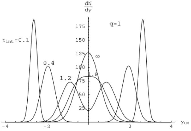
-4 -2 2 4 yCM 25
50 75 100 125 150 175 dN
dy
Τint=0.1
0.4
1.2 ¥
q=1
1.8
Figure 1. Shape of the rapidity distribution at different integration timeτintfor the undeformed case (q= 1).
The obtained spectra are normalized to 164 protons and the beam rapidity is fixed toycm = 2.9(in the c.m. frame)
[13]. In Fig. 1, we show the shape of the rapiditity distrib-ution at different integration timeτint of the linear Fokker-Planck equation (q = 1). In Fig. 2, we report the time evo-lution of the rapidity distribution corresponding to the inte-gration of the NLFPE with q = 1.25(the value of the q -parameter used to fit the data).
-4 -2 2 4 yCM
10 20 30 40 50 dN dy
Τint=0.1
0.4
1 ¥
q=1.25
1.2
Figure 2. The same of Fig. 1 forq= 1.25
In Fig. 3, we show the calculated rapidity spectra com-pared with the experimental data. The full line corresponds to the NLFPE solution (58) at τint = 0.82andq = 1.25; the dashed line corresponds to the solution of the linear case (q = 1) atτint = 1.2. Imposing the validity of the fluctuation-dissipation theorem, it is not possible to repro-duce the experimental rapidity shape at any time. Only in the non-linear case (q6= 1) exists a (finite) time for which the obtained rapidity spectra well reproduces the broad experi-mental shape. A value ofq6= 1implies anomalous superdif-fussion in the rapidity space, i.e.,[y(t)−yM(t)]2scale like
tαwithα >1[12].
A complete description of the applicability of nonexten-sive statistical effects to high-energy heavy ion collisions lies out the scope of this paper. However, we want to outline that an analysis of the transverse pion momentum spectra and the
net proton rapitity distribution measured at RHIC is under in-vestigation.
-3 -2 -1 1 2 3 yCM
20 40 60 80 dN
dy
q=1, Τ=1.2
q=1.25, Τ=0.82
Figure 3. Rapidity spectra for net proton production (p−p) in
cen-tral Pb+Pb collisions at 158A GeV/c (grey circles are data reflected aboutycm= 0) [13]. Full line corresponds to our results by using a
non-linear evolution equation (q = 1.25), dashed line corresponds
to the linear case (q= 1)
6
Conclusion
There is an increasing evidence that the generalized nonex-tensive thermodynamics can be considered as the more ap-propriate basis of a theoretical framework to deal with several physical phenomena where range interactions, long-range memory effects and/or fractal space-time constraints are present. A considerable variety of physical applications involve microscopic quantum and/or relativistic effects. The main effort of this paper is to study an appropriate generaliza-tion of the quantum dynamics and relativistic kinetic equageneraliza-tion in the framework of the Tsallis nonextensive thermostatistics. We have introduced two kinds of generalized Schr¨odinger equations which satisfy the basic assumptions of the quan-tum mechanics under appropriate operator properties which depend on the deformation parameter q. Furthermore, we have studied a nonextensive generalization of the relativis-tic Boltzmann equation and of the nonlinear Fokker-Planck equation. The above evolution equations have been applied to the study of the nonequilibrium rapidity distribution in rela-tivistic heavy-ion collisions obtaining a very good agreement with the experimental results.
References
[1] C. Tsallis, J. Stat. Phys. 52, 479 (1988). See also http://tsallis.cat.cbpf.br/biblio.htm for a regularly updated bib-liography on the subject.
[2] C. Tsallis, R.S. Mendes, and A.R. Plastino, Physica A261, 534 (1998).
[3] S. Mart´ınez, F. Nicol´as, F. Pennini, and A. Plastino, Physica A
[4] S. Mart´ınez, F. Pennini, and A. Plastino, Phys. Lett. A278, 47 (2000).
[5] L. Borland, Phys. Lett. A245, 67 (1998).
[6] W.M. Alberico, A. Lavagno, and P. Quarati, Eur. Phys. J. C12, 499 (2000); Nucl. Phys. A680, 94c (2001).
[7] A. Lavagno, Phys. Lett. A301, 13 (2002).
[8] A. Drago, A. Lavagno, and P. Quarati, Physica A344, 472 (2004).
[9] S.R. Groot, W.A. van Leeuwen, and Ch. G. van Weert, Relati-vistic Kinetic Theory(North-Holland, Amsterdam, 1980). [10] J.A.S. Lima, R. Silva, and A.R. Plastino, Phys. Rev. Lett.86,
2938 (2001).
[11] G. Wolschin, Eur. Phys. J. A5, 85 (1999); Phys. Rev. C69, 024906 (2004).
[12] C. Tsallis, D.J. Bukman, Phys. Rev. E54, R2197 (1996). [13] H. Appelsh¨auser et al. (NA49 Collaboration), Phys. Rev. Lett.
82, 2471 (1999).
[14] I.G. Bearden et al. (NA44 Collaboration), Phys. Rev. Lett.78, 2080 (1997).
[15] P. Braun-Munzinger et al., Phys. Lett. B344, 43 (1995); B
356, 1 (1996).