Rapidity Dependence of HBT Radii Based on a Hydrodynamical Model
Kenji Morita1∗
1 Department of Physics, Waseda University, Tokyo 169-8555, Japan Received on 10 November, 2006
We calculate two-pion correlation functions at finite rapidities based on a hydrodynamical model which does
not assume explicit boost invariance along the collision axis. Extracting the HBT radii throughχ2fits in both
Cartesian and Yano-Koonin-Podgoretski˘ı parametrizations, we compare them with experimental results from the PHOBOS collaboration. Based on the results, we discuss longitudinal expansion dynamics.
Keywords: Hydrodynamical model; Pion interferometry; Boost invariance
I. INTRODUCTION
“Perfect fluidity” of the matter created at the Relativistic Heavy Ion Collider (RHIC) at BNL is some of the most excit-ing news in the field of high energy nuclear physics [1]. Ex-perimental results and their comparison with theoretical cal-culation reveal that the matter created in Au+Au collisions should be something like a liquid of quarks and gluons, un-like a gas of almost free partons as naively expected [2]. One strong piece of evidence for this finding is the observation of large elliptic flow (v2) and its agreement with a perfect fluid-dynamical calculation [3]. In order to reproduce the experi-mental result with such models, an equation of state assuming a partonic state at high temperature and a phase transition and rapid thermalization time (τ0≤1fm/c) are required [3]. The hydrodynamic model based on numerical solutions of the rela-tivistic hydrodynamic equation for perfect fluid has become an indispensable tool for theoretical analyses of relativistic heavy ion collisions. Furthermore, the model itself has been becom-ing more sophisticated in order to reproduce new experimen-tal data with higher statistics. Currently, the most sophisti-cated calculations model a full three-dimensional (solving hy-drodynamic equation without any symmetry) hyhy-drodynamic expansion followed by a hadronic cascade [4, 5]. These mod-els can reproduce most soft hadronic observables. Especially, the simultaneous description of particle ratios, transverse mo-mentum spectra and elliptic flow is possible with such hybrid models.
However, there are still some insufficient ingredients in the hydrodynamic analyses. First, we don’t have reasonable ini-tial condition derived from first principles. Recently, the Color Glass Condensate (CGC) has been proposed as a suitable ini-tial condition for relativistic heavy ion collisions [6]. This picture has been examined as an initial condition for a hydro-dynamic model in Ref. [7] and found to give a good descrip-tion of some observables in the case of fully hydrodynamic description of the collision process. However, this initial con-dition fails if one takes hadronic dissipation into account [4]. This fact suggests there is still open space for a dissipative partonic phase, or improvement of the initial condition.
∗Present Address: Institute of Physics and Applied Physics, Yonsei
Univer-sity, Seoul 120-749, Korea
Second, the equation of state (EoS) of QCD matter has not yet been fully understood. Since one of the most important merit of using a hydrodynamic model is that it can be directly related to the EoS, detailed information on the EoS for all re-gion of temperature and baryonic chemical potential is indis-pensable. As for RHIC energies, the net baryon number ob-served at midrapidity is small enough to neglect it [8]. Never-theless, the EoS at finite baryonic chemical potential may play an important role in the forward rapidity region and in heavy ion collisions at lower energies. Because of the well-known difficulty of lattice QCD at finite baryonic chemical poten-tial [9], lattice QCD calculations have not yet provided the complete solution. For vanishing baryonic chemical potential, the lattice equation of state clearly shows a different behavior from the free parton gas [10], and a lattice-inspired EoS has been implemented in hydrodynamic calculations [11].
At last, in spite of the success in most soft observables, re-sults of the two-pion momentum intensity correlation from such hydrodynamical models do not yet agree with experi-mental data. According to the symmetry of the wave function of two identical bosons, the two-particle correlation function can be related to sizes of the source from which particles are emitted. This fact is known as Hanbury Brown-Twiss (HBT) effect. Because it concerns source sizes, which depend on mo-mentum of particle pairs due to collective flow, the pion corre-lation function is a diagnostic tool for the space-time evolution of the matter. Since the disagreement was first found with a (2+1)-dimensional model with boost invariance along the col-lision axis [12], many extensions such as an explicit longitu-dinal expansion [13, 14], incorporating chemical freeze-out [14], chiral model EoS [15], an opaque source [16], fluctu-ating initial conditions and continuous freeze-out [17], have been examined. The discrepancy has been reduced, but the situation is still unsatisfactory. There are various possibilities for further improvements.
the symmetry. This radius contains information on the corre-lation between freeze-out points on the transverse plane and those on the longitudinal direction. Hence, it is expected that this quantity is sensitive to longitudinal expansion dynamics beyond the boost-invariant approximation. Similar consider-ations also hold for the Yano-Koonin-Podgoretski˘ı parame-trization which has three radius parameters and one velocity parameter called YK velocity [22, 23]. The PHOBOS data also provide rapidity dependence of the YKP radii and YK ve-locity [18], which may impose a restriction on the longitudinal expansion dynamics. Indeed, the initial matter distribution as an input for hydrodynamic calculations has not yet been fixed. This is indicated by Hirano in Ref. [24], in which two different initial energy density distributions result in reasonable agree-ment with experiagree-mental data of pseudorapidity distribution of charged hadrons measured in 130AGeV Au+Au collisions at RHIC.
In this work, we employ two different initial energy density distributions for the hydrodynamic equations, as in Ref. [24]. We focus our discussion on central collisions. Both of them are tuned so that they reproduce the pseudorapidity distribu-tion of charged hadrons measured in the most central events at 200AGeV Au+Au collisions. Then, we compare the space-time evolution and shape of the freeze-out hypersurface of the fluids and see how the difference in the initial condition is re-flected onto them. We calculate the two-pion correlation func-tion as the most promising experimental observable to see the difference. Extracting the HBT radii through Gaussian fits, we compare them with the experimental results and discuss the transverse momentum and rapidity dependence of the HBT radii. In the next section, we briefly review the hydrodynam-ical model used in this work. Initial conditions are given in Sec.III. In Sec. IV, we show numerical solutions of hydrody-namical equations for the initial conditions given in Sec. III. Results for the HBT radii as compared with the experimental data are given in Sec. V. Section VI is devoted to a summary.
II. HYDRODYNAMICAL MODEL
The basic equation of hydrodynamical models is the energy-momentum conservation law
∂µTµν=0, (1)
whereTµνis the energy-momentum tensor. For a perfect fluid, Tµν= (ε+P)uµuν−Pgµν, (2) wheregµν=diag(+,−,−,−)andε,Panduµare the energy density, pressure and the four velocities of the fluid, respec-tively. If one takes a conserved chargeisuch as baryon num-ber and strangeness into account, the conservation law
∂µ(niuµ) =0 (3)
is added. Providing an EoSP=P(ε,ni), one can solve these coupled equations numerically.
In this work, we consider the baryon number charge as a conserved charge and adopt an equation of state which ex-hibits a first order phase transition on the phase boundary in
theT−µBplane from the free massless partonic gas with three flavors to the free resonance gas which consists of hadrons ex-cept for hyperons up to 2 GeV/c2of mass with excluded vol-ume correction[25]. See Ref.[26] for the detail. The critical temperatureTcat vanishing baryonic chemical potential is set to 160 MeV. This model is basically same as the one used in Refs. [13, 16].
Defining thez-axis as the collision axis, we use a cylindrical coordinate system(τ,ηs,r,φ)as follows;
t=τcoshηs, (4)
z=τsinhηs, (5)
rx=rcosφ, (6)
ry=rsinφ. (7)
Here, τ=√t2−z2 is the proper time and ηs=1/2 ln[(t+
z)/(t−z)]is the space-time rapidity. Since we focus on cen-tral collisions, we assume an azimuthally symmetric system. Then, by virtue ofuµuµ=1, the four velocities are given in terms of a longitudinal flow rapidityYLand a transverse flow rapidityYTas
uτ=cosh(YL−ηs)coshYT, (8)
uηs=sinh(Y
L−ηs)coshYT, (9)
ur=sinhYL. (10)
To solve the equations numerically, we employed a method based on the Lagrangian hydrodynamics which traces flux of the current. The numerical procedure is described in Ref. [27]. For treatment of the first order phase transition, we introduce a fraction of the volume of the QGP phase to express the energy density and net baryon number density at the mixed phase [26]. In this algorithm, we explicitly solve the entropy and baryon number conservation law. We checked that these quantities are conserved throughout the numerical calculation within 1% accuracy for a time stepδτ=0.01 fm/c, by choos-ing proper mesh sizes ofηsandrdirections.
III. INITIAL CONDITIONS
Firstly, we choose an initial proper time asτ0=1 fm/c. Initial values for other variables are given on this hyper-bola. Longitudinal flow rapidity is set to the Bjorken’s scaling ansatzYL=ηs [28]. Transverse flow is simply neglected at the initial proper time [29]. For the matter distributions, we assume that the energy and baryon number density are pro-portional to the number of binary collisions. Hence, for the Woods-Saxon profile of the nucleon density in nuclei,
ρW(r,z) = ρ0
e(√r2+z2−R)/ξ
+1
, (11)
whereR=1.12A1/3−0.86A−1/3fm is the radius of the nu-clear with mass numberA,ξ=0.54 fm is the surface diffuse-ness andρ0is the normal nuclear matter density, the density of binary collisions at vanishing impact parameter is given by
nBC(r) =σ0
∞
−∞
dzρW(r,z)
2
withσ0being the total inelastic nucleon-nucleon cross section which is absorbed into the proportionality constant between nBCand matter distributions.
Then, the energy density distribution is parameterized with a “flat+Gaussian” form,
ε(τ0,ηs,r) =ε0exp
−(|ηs| −ηs0) 2
2σ2 ηs
θ(|ηs| −ηs0)
nBC(r). (13) Here, nBC(r) is the normalized density of binary collisions (12), ε0 the maximum energy density, andηs0 andσηs are parameters which determine the length of the flat region and width of the Gaussian part, respectively. Similarly, the net baryon number density distribution is parameterized as
nB(τ0,ηs,r) =nB0
exp
−(|ηs| −ηsD) 2
2σ2 sD
θ(|ηs| −ηs0)
+exp
−(ηs0−ηsD) 2
2σ2 sD
θ(ηs0− |ηs|)
nBC(r), (14) wherenB0 is the maximum net baryon number density and ηsDandσsDare the shape parameters as in Eq. (13).
To calculate final particle distribution, we use the Cooper-Frye prescription [30]. The pseudorapidity distribution for a particle speciesiis given by
dNi dη =
di
(2π)2 ∞
0
dkt kt|k|
k0
Σ
k·dσf(k·u,T,µB), (15) wherekµis the momentum of thermally produced particlesi withdibeing the number of degrees of freedom, the pseudo-rapidity η defined by η=1/2 ln[(|k|+kz)/(|k| −kz)], and f(k·u,T,µB)describing the the equilibrium distribution func-tions. We take into account not only directly produced par-ticles but also resonance decay contributions. The freeze-out hypersurface Σis defined by picking a constant temper-ature,T =Tf=140 MeV. Here, we assume that thermal and chemical freeze-out occur simultaneously. Since experimen-tal data of particle yields can be well described by the statisti-cal model with high chemistatisti-cal freeze-out temperature close to Tc [31], we cannot reproduce the correct particle yields with this lower freeze-out temperature. However, in hydrodynamic analyses,ktspectra are sensitive to the thermal freeze-out tem-perature, which affects the transverse expansion. In this calcu-lation, we set the freeze-out temperature so that pionkt spec-trum is roughly reproduced in IC B and set the same out temperature for IC A and IC B. Note that the freeze-out temperature depends on the choice of the transverse pro-file of the initial matter distribution because a steeper pres-sure gradient yields larger transverse flow. For example, even Tf≃150−160 MeV is possible with an initialization based on pQCD+saturation model [32]. Our value is only slightly different from Ref. [24], where the initial profile is very sim-ilar. In order to reproduce both the particle yields and the kt spectra in dynamical regimes, one should introduce sepa-rate freeze-out temperatures [14, 33] or go to hybrid approach [4, 5, 34, 35]. In this work, however, our main argument will not be so affected by the description of the freeze-out because we focus on longitudinal expansion.
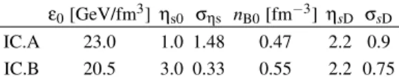
TABLE I: Parameters in initial matter distributions.
ε0[GeV/fm3] ηs0 σηs nB0[fm−3] ηsD σsD
IC.A 23.0 1.0 1.48 0.47 2.2 0.9
IC.B 20.5 3.0 0.33 0.55 2.2 0.75
In Table I, two sets of the initial parameters are listed. The corresponding initial energy density distributions, resultant pseudorapidity distributions and transverse momentum distri-butions are illustrated in Fig. 1, 2 and 3, respectively. We have chosen two initial conditions, both of which reproduce the experimental data of PHOBOS for the pseudo-rapidity distribution of charged hadrons [36], and of PHENIX for the transverse momentum distributions ofπ−,K−and ¯p[37], and of BRAHMS for the rapidity distribution of net protons [38]. These two initial conditions are characterized by two parame-ters,ηs0andσs0. One has smallηs0and largeσs0, which we denote initial condition A (IC.A). The other, which we rep-resent IC.B, has the opposite feature;ηs0 is large andσs0is small. The initial energy densities are both much larger than experimental estimations (∼5 GeV/fm3) based on Bjorken’s formula [2], but note thatε0in Table I is not anaverageenergy density butmaximumenergy density, which strongly depends on the profile of initial matter distributions [39]. We calcu-lated pseudorapidity distributions for not only these two ini-tial conditions, but also for intermediate ones by varyingηs0 from 1.0 to 3.0, and found that they can also reproduce the ex-perimental data by adjusting other parameters appropriately. Perhaps the best fit will exist in the middle of this parameter range [40]. Here, we choose the extreme cases in order to see differences in the space-time evolution of the fluids originat-ing from the difference in the initial conditions.
IV. SPACE-TIME EVOLUTION OF THE FLUIDS
Figures 4 and 5 show the space-time evolution of the tem-perature distributions and deviation from the scaling solution YL=ηs, as a function ofηsatr=0 for variousτ, respectively. From these figures, we find that the space-time evolution at forward rapidity is quite different between IC.A and IC.B in spite of the fact that both solutions give similar pseudorapid-ity distributions of hadrons. In IC.B, the sharp decrease of temperature, which is identical to steep pressure gradient at forward rapidity, causes rapid acceleration of the longitudinal flow at the edge of the fluid. On the other hand, in IC.A, pres-sure gradient is rather gradual. Hence, the resultant deviation from the scaling solution is smaller. However, because pres-sure gradients exist at smallerηsin IC.A, such deviations take place atηs≃1 while the flow maintains the scaling solutions up toηs≃2 in IC.B. This fact explains the slightly largerε0 in IC.A since faster longitudinal expansion than the scaling expansion pushes entropy per unit rapidity to forward rapidity [13, 41].
0 1 2 3 4 5 0 2
4 6 0 5 10 15 20 25
ε[GeV/fm3]
ηs0=1.0,ση
s=1.48
ηs
r [fm]
ε[GeV/fm3]
0 1 2 3 4 5 0 2
4 6 0 5 10 15 20 25
ε[GeV/fm3]
ηs0=3.0,ση
s=0.33
ηs
r [fm]
ε[GeV/fm3]
IC.A IC.B
FIG. 1: Initial energy density distributions
0 100 200 300 400 500 600 700 800
-4 -2 0 2 4
dN/d η Pseudorapidityη IC.A IC.B PHOBOS
FIG. 2: Pseudorapidity distribution. The solid line and dashed line stand for the initial conditions A and B, respectively. Experimental data measured by PHOBOS are taken from Ref.[36].
1e-005 0.0001 0.001 0.01 0.1 1 10 100 1000
0 0.5 1 1.5 2 2.5 3 3.5 4
1/2
π
kT
dN/dk
T
dY [arb. units]
kT [GeV/c] π
-K
-
p-IC A, π -IC B, π -PHENIXπ -IC A, K -IC B, K -PHENIX K -IC A, IC B, PHENIX
p-FIG. 3: Transverse momentum distribution of identified negatively charged hadrons. Spectra for kaons and anti-protons are scaled by factors 0.1 and 0.01 for a clear comparison of the slopes, respectively. Experimental data measured by PHENIX are taken from Ref. [37]. Identification of symbols is same as Fig. 2.
ial that such differences can survive at the freeze-out hypersur-faces. Since hadrons strongly interact and provide informa-tion only at thermal freeze-out, differences in the freeze-out hypersurfaces are necessary to lead to a signature in hadronic experimental observables.
We show the freeze-out proper timeτfof all fluid elements in Fig. 6. This characterizes the shape of the freeze-out hyper-surface, which is expected to affect the HBT radii. In Fig. 6,
150 200 250 300 350
0 1 2 3 4 5
Temperature T [MeV]
Space-time rapidity ηs
IC.A
τ=1 fm/c
τ=3 fm/c
τ=5 fm/c
τ=7 fm/c
τ=9 fm/c
τ=11 fm/c
τ=13 fm/c
150 200 250 300 350
0 1 2 3 4 5
Temperature T [MeV]
Space-time rapidity ηs
IC.B
τ=1 fm/c
τ=3 fm/c
τ=5 fm/c
τ=7 fm/c
τ=9 fm/c
τ=11 fm/c
τ=13 fm/c
FIG. 4: Space-time evolution of temperature distributions atr=0.
0 0.2 0.4 0.6 0.8
0 1 2 3 4 5
YL
-ηs
Space-time rapidity ηs
IC.A
τ=1 fm/c
τ=3 fm/c
τ=5 fm/c
τ=7 fm/c
τ=9 fm/c
τ=11 fm/c
τ=13 fm/c
-0.1 0 0.1 0.2 0.3 0.4 0.5 0.6 0.7 0.8 0.9
0 1 2 3 4 5
YL
-ηs
Space-time rapidity ηs
IC.B
τ=1 fm/c
τ=3 fm/c
τ=5 fm/c
τ=7 fm/c
τ=9 fm/c
τ=11 fm/c
τ=13 fm/c
FIG. 5: Deviation from the scaling solution atr=0.
0 1
2 3
4
5 1 2 3 4 5 6 7 8 15
10 5 1
τf [fm/c]
IC.A
ηs r [fm]
τf [fm/c]
0 1
2 3
4
5 1 2 3 4 5 6 7 8 15
10 5 1
τf [fm/c]
IC.B
ηs r [fm]
τf [fm/c]
FIG. 6: Freeze-out hypersurface of the fluids.
0 1 2 3
4 5 0 1 2 3
4 5 6 7
8 0
0.2 0.4 0.6 YL-ηs
ηs
r [fm] YL-ηs
0 1 2 3
4 5 0 1 2 3
4 5 6 7
8 0
0.2 0.4 0.6 YL-ηs
ηs
r [fm] YL-ηs
FIG. 7: Deviation from the scaling solution on the freeze-out hyper-surfaces.
how these differences affect the HBT radii in the next section.
V. HBT RADII
A. Two-pion correlation function
Assuming that the source is completely chaotic, we can cal-culate the two-particle correlation momentum intensity corre-lation function through this formula [42]
C2(q,K) =1+ |
I(q,K)|2
I(0,k1)I(0,k2)
, (16)
where q=k1−k2 is the four-relative momentum and K= 1/2(k1+k2) is the four-average momentum, with ki being on-shell momentum of emitted pions. The interference term I(q,K)can be chosen as
I(q,K) =
ΣK·dσe iq·xf(u
·K,T), (17)
so thatI(0,ki)reduces to the Cooper-Frye formula [43]. Experimentally, the two-pion correlation function is de-fined as
C2(q) =
A(q)
B(q), (18)
whereA(q) is the measured two-pion pair distribution with momentum difference q, and B(q) is the background pair distribution generated from mixed events. Momentum ac-ceptances are imposed separately in the numerator and the denominator. Accounting for the large acceptance in the PHOBOS experiment, 0.4<Yππ<1.3 for threeKTbins and 0.1<KT<1.4 GeV/cfor three rapidity bins, we integrate the correlation function as follows:
C(q;KT) =1+ 1.3
0.4dYππ|I(q,K)|2 1.3
0.4dYππI(0,k1)I(0,k2)
, (19)
C(q;Yππ) =1+ 1.4
0.1dKTKT|I(q,K)|2 1.4
0.1dKTKTI(0,k1)I(0,k2)
. (20)
For simplicity, we consider only directly emitted pions and neglect resonance decay contributions.
B. KTdependence of the HBT radii in the Cartesian
parametrization
Physical meaning of the HBT radii depends on the choice of three independent components of the relative momentum q. The most standard choice is the so-called Cartesian Bertch-Pratt parametrization [19, 20]q= (qout,qside,qlong)in which “long” means parallel to the collision axis, “side” perpendicu-lar to the transverse component of the average momentumKT and “out” parallel toKT. In the case of azimuthally symmet-ric system as considered here, one can putKT= (KT,0) so thatqout=qxandqside=qy. Note thatqlong=qz. Then, the
Gaussian form of the two-pion correlation function is given as [21]
C2fit(q) =1+λexp(−q2outR2out−q2sideR2side−q2longR2long
−2qoutqlongR2ol). (21)
The HBT radiiRi can be extracted by a χ2-fit to the above fitting function. For a chaotic source, the chaoticity parame-terλshould become unity. However, the experimentally ob-served chaoticity is smaller than 1 because of such contribu-tions as long-lived resonance decay [44]. Here we fixλ=1 in the Gaussian fit to the calculated correlation functions with Eqs. (19) and (20).
By expanding the correlation function (16) for q·x≪1, the size parametersRican be related to second order moments of the source function [21]. In the Cartesian parametrization, taking the longitudinal co-moving system (LCMS) makes the expression simple;
R2out=(r˜x−β⊥t˜)2
=r˜x2 −2β⊥r˜xt˜ +β2⊥t˜2 . (22)
R2side=r˜y2 , (23)
R2long=z˜2 , (24)
R2ol=(r˜x−β⊥t˜)z˜ , (25) where
A(x) ≡
Σk·dσf(u·k,T)A(x)
Σk·dσf(u·k,T)
, (26)
˜
x≡x− x , and β⊥=kT/Ek. Hence, Rout, Rside andRlong can be interpreted as a mixture of the thickness of the source and the emission duration, the transverse source size, and the longitudinal source size, as seen from the LCMS, respectively. The validity of these expressions for a hydrodynamical model is discussed in Ref. [45]. Although they have been shown to be good approximations, it is also pointed out that there are still some discrepancies, and one should use fitted HBT radii for comparison with the experimental data which are obtained from the fit [46].
Figure 8 shows results for the four HBT radii compared with the experimental data measured by PHOBOS [18]. For comparison of the initial conditions, any qualitative and quan-titative difference cannot be seen inRoutandRside, as expected from Fig. 6. Rlongof IC.A is about 1 fm smaller than that of IC.B. This can be considered as a consequence of the fact that the deviation from the scaling solution at smallηsis larger in IC.A, because faster flow causes more thermal suppression of the emission region [13]. For these three radii, our calcula-tion cannot reproduce the experimental results and show sim-ilar behavior with other perfect fluid dynamical calculations of Ref.[12–14, 16]. EspeciallyRlongshows the largest devi-ation from experimental data, although the calculdevi-ation is im-proved by including longitudinal expansion without explicit boost invariance [13, 14]. In the bottom of Fig. 8, the result of the out-long cross term is presented. Reflecting the uniform shape of the freeze-out hypersurface in Fig. 6, the value ofR2
0 2 4 6 8 10
0 0.2 0.4 0.6 0.8
Rout
[fm]
KT [GeV/c] IC.A IC.B
PHOBOSπ
-PHOBOSπ+
0 2 4 6 8 10
0 0.2 0.4 0.6 0.8
Rside
[fm]
KT [GeV/c] IC.A IC.B
PHOBOSπ
-PHOBOSπ+
0 2 4 6 8 10
0 0.2 0.4 0.6 0.8
Rlong
[fm]
KT [GeV/c] IC.A IC.B
PHOBOSπ
-PHOBOSπ+
-2 0 2 4 6 8 10
0 0.2 0.4 0.6 0.8
Rol 2 [fm 2 ]
KT [GeV/c] IC.A IC.B
PHOBOSπ
-PHOBOSπ+
FIG. 8:KTdependence of Cartesian HBT radii. Closed squares and
open squares denote our results for IC.A and IC.B, respectively. Ex-perimental data are taken from Ref. [18]. Error-bars for the experi-mental data are statistical only.
of IC.B is smaller than that of IC.A. At the lowestKTbin, the difference is about 4 fm2. Unfortunately, experimental uncer-tainty is still too large to distinguish which initial condition is favored. However, it should be noted that both of two results agree with the experimental data, in spite of the disagreement of other radii.
C. Rapidity dependence of the HBT radii in the YKP parametrization
In the YKP parametrization, three independent components of the relative momentumq are q⊥= q2
x+q2y,q=qz = qlongandqτ=E1−E2. Then, the Gaussian fitting correlation function is given as
C2YKP(q) =1+λexp
−R2⊥q2⊥−R2(q2−q2τ)
−(R2τ+R2)(q·U)2, (27)
whereUµ=γ(1,0,0,vYK), γ=1/ 1−v2YK andvYK is the fourth fitting parameter called the YK velocity. The three HBT radii,R⊥,RandRτare invariant under a longitudinal boost. Physical meaning of the parameters can be given in a similar manner [23] and becomes the simplest as follows, if one adopt the YK frame wherevYK=0,
R2⊥=r˜y2 =R2side, (28)
R2≃ z˜2 =R2long, (29)
R2τ≃ t˜2 . (30)
The main advantage of using YKP parametrization is that the three HBT radii directly give the transverse, longitudinal and temporal source size, that are seen from the YK frame. How-ever, one should note that the latter two, (29) and (30), are approximate expressions which hold only if the source is not opaque [45]. Hence, R andRτ cannot be always regarded as the source sizes in the presence of strong transverse flow which makes the source highly opaque [16]. The general ex-pression ofvYKis complicated one [23] but it can be regarded as a longitudinal flow velocity of the source measured in an observer’s frame.
0 2 4 6 8 10
0 1 2 3 4
R⊥
[fm]
Yππ
IC.A IC.B
PHOBOSπ
-PHOBOSπ+
0 2 4 6 8 10
0 1 2 3 4
R||
[fm]
Yππ IC.A IC.B
PHOBOSπ
-PHOBOSπ+
0 2 4 6 8 10
0 1 2 3 4
Rτ
[fm]
Yππ
IC.A IC.B
PHOBOSπ
-PHOBOSπ+
FIG. 9: HBT radii for the YKP parametrization. The identification of the symbols is the same as in Fig. 8.
a possible origin of the deviation of our result from the data is larger emission duration. Some model calculations based on source parametrization [48] and parametric exact solution of hydrodynamics [49] show very small emission duration time, 0-2 fm/cin agreement with data on the bottom panel of Fig. 9. We cannot see any significant differences in the HBT radii at forward rapidity expected from Figs. 6 and 7 which display the differences of the source shape and the longitudinal flow. This will come from the fact that the number of produced par-ticles is larger at late freeze-out proper time in the case of the current freeze-out condition [45].
Finally, the Yano-Koonin rapidity YYK = 1/2 ln[(1+
vYK)/(1−vYK)]is shown as a function ofYππin Fig. 10. Both results from IC.A and IC.B surprisingly agree with the
exper-imental data and show no difference between the two. In the forward rapidity region, our results show deviation from the infinite boost invariant case, which is indicated by the straight line. Although our solutions of longitudinal flow show devia-tion from the scaling soludevia-tion (Figs. 5 and 7), the result would have to yieldYYKlarger than a givenYππ, ifYYKcorrectly rep-resents the longitudinal source velocity. Hence, this deviation will be caused by the finite size effect [45] which becomes more significant at forward rapidity rather than the difference in the flow velocity.
0 1 2 3 4
0 1 2 3 4
YYKP
Yππ IC.A IC.B PHOBOSπ -PHOBOSπ+
FIG. 10: The Yano-Koonin rapidityYYK. The identification of the
symbols is the same as in Figs. 8 and 9. The solid line indicates the case of the infinite boost-invariant source.
VI. SUMMARY
then Rlong andR. We used the conventional Cooper-Frye prescription for the out. Improvement of the freeze-out prescription by continuous freeze-freeze-out [11] and hybrid ap-proach [4, 5] can yield largerRsidebut this may lead to larger
Routbecause of extended emission duration. Nevertheless, as a transport calculation [50] shows, positivex−tcorrelation in the source function may resolve this problem. Finally, in spite of the disagreement of the HBT radii, the YK rapidity shows a good agreement with the experimental data. Our calculation predicts some deviations at larger rapidities from the infinite boost-invariant case. Hence, measurements at this region is
needed for further understanding of the expansion dynamics.
Acknowledgements
The author is indebted to Profs. I. Ohba and H. Nakazato for their encourgement. He also would like to thank S. Muroya and T. Hirano for their helpful discussions. This work was supported by a Grant for the 21st Century COE Pro-gram at Waseda University from Ministry of Education, Cul-ture, Sports, Science and Technology of Japan. This is also supported by BK21 (Brain Korea 21) program of the Korean Ministry of Education.
[1] http://www.bnl.gov/bnlweb/pubaf/pr/PR display.asp? prID=05-38
[2] I. Arseneet al., (BRAHMS Collaboration), Nucl. Phys. A757,
1 (2005); B. B. Backet al., (PHOBOS Collaboration),ibid, A
757, 28 (2005); J. Adamset al., (STAR Collaboration), ibid,
A757, 102 (2005); K. Adcoxet al., (PHENIX Collaboration),
ibid, A757, 184 (2005).
[3] P. F. Kolb, P. Huovinen, U. Heinz, and H. Heiselberg,
Phys. Lett. B500, 232 (2001).
[4] T. Hirano, U. Heinz, D. Kharzeev, R. Lacey, and Y. Nara,
Phys. Lett. B636, 299 (2006).
[5] C. Nonaka, S. A. Bass, arXiv:nucl-th/0607018.
[6] E. Iancu, R. Venugopalan, inQuark-Gluon Plasma 3, edited by
R. C. Hwa, X. N. Wang, World Scientific, Singapore, 2004.
[7] T. Hirano and Y. Nara, Nucl. Phys. A743, 305 (2004).
[8] I. G. Bearden et al., (BRAHMS Collaboration),
Phys. Rev. Lett.93, 102301 (2004).
[9] For a review, S. Muroya, A. Nakamura, C. Nonaka, and
T. Takaishi, Prog. Theor. Phys.110, 615 (2003).
[10] Y. Aoki, Z. Fodor, S. D. Katz, and K. K. Szabo, JHEP0601,
089 (2006).
[11] Y. Hama, R. P. G. Andrade, F. Grassi, O. Socolowski Jr., T.
Ko-dama, B. Tavares, and S. S. Padula, Nucl. Phys. A774, 169
(2006).
[12] U. Heinz, P. Kolb, Nucl. Phys. A702, 269 (2002).
[13] T. Hirano, K. Morita, S. Muroya, and C. Nonaka, Phys. Rev. C
65, 061902(R) (2002); K. Morita, S. Muroya, C. Nonaka, and
T. Hirano,ibid.,66, 054904 (2002).
[14] T. Hirano, K. Tsuda, Phys. Rev. C66, 054905 (2002).
[15] D. Zschiesche, H. St¨ocker, W. Greiner, and S. Schramm,
Phys. Rev. C65, 064902 (2002).
[16] K. Morita, S. Muroya, Prog. Theor. Phys.111, 93 (2004).
[17] O. Socorowski,Jr., F. Grassi, Y. Hama, and T. Kodama,
Phys. Rev. Lett.93, 182301 (2004).
[18] B. B. Backet al., (PHOBOS Collaboration), Phys. Rev. C73,
031901(R) (2006).
[19] G. Bertsch, M. Gong, and M. Tohyama, Phys. Rev. C37, 1896
(1988).
[20] S. Pratt, T. Cs¨org˝o, and J. Zim´anyi, Phys. Rev. C 42, 2646
(1990).
[21] S. Chapman, P. Scotto, and U. Heinz, Phys. Rev. Lett.74, 4400
(1995).
[22] F. Yano, S. Koonin, Phys. Lett. B78, 556 (1978); M. I.
Pod-goretski˘ı, Sov. J. Nucl. Phys.37, 272 (1983).
[23] Y. -F. Wu, U. Heinz, B. Tom´aˇsik, and U. A. Wiedemann,
Eur. Phys. J. C1, 599 (1998).
[24] T. Hirano, Phys. Rev. C65, 011901(R) (2001).
[25] Note that, however, this EoS does not agree with recent lattice
QCD calculations which exhibit cross-over transition at
vanish-ing and smallµB[10].
[26] C. Nonaka, E. Honda, and S. Muroya, Eur. Phys. J. C17, 663
(2000).
[27] T. Ishii, S. Muroya, Phys. Rev. D46, 5156 (1992).
[28] J. D. Bjorken, Phys. Rev. D27, 140 (1983).
[29] Note that the existence of the initial transverse flow can improve results for transverse momentum spectra but is an open issue. In this work, however, we simply neglect it in order to avoid to add additional parameters such as flow strength and profile. Since we are mainly focusing on longitudinal expansion dynamics in this paper, this simplification will not affect our main argument.
[30] F. Cooper and G. Frye, Phys. Rev. D10, 186 (1974).
[31] P. Braun-Munzinger, D. Magestro, K. Redlich, and J. Stachel,
Phys. Lett. B518, 41 (2001).
[32] K. J. Eskola, H. Niemi, P. V. Ruuskanen, and S. S. R¨as¨anen,
Phys. Lett. B566, 187 (2003).
[33] P. F. Kolb, R. Rapp, Phys. Rev. C67, 044903 (2003).
[34] S. A. Bass, A. Dumitru, Phys. Rev. C61, 064909 (2000).
[35] D. Teaney, J. Lauret, and E. V. Shuryak, Phys. Rev. Lett.86,
4783 (2003).
[36] B. B. Backet al., (PHOBOS Collaboration), Phys. Rev. Lett.
91, 052303 (2003).
[37] S. S. Adleret al., (PHENIX Collaboration), Phys. Rev. C69,
034909 (2004).
[38] I. G. Beardenet al., Phys. Rev. Lett.93, 102301 (2004).
[39] P. F. Kolb, U. Heinz, P. Huovinen, K. J. Eskola, and K.
Tuomi-nen, Nucl. Phys. A696, 197 (2001).
[40] L. M. Satarov, A. V. Merdeev, I. N. Mishustin, and H. St ¨ocker,
arXiv:hep-ph/0606074 .
[41] K. J. Eskola, K. Kajantie, and P. V. Ruuskanen, Eur. Phys. J. C
1, 627 (1998).
[42] E. V. Shuryak, Phys. Lett. B44, 387 (1973).
[43] S. Chapman, U. Heinz, Phys. Lett. B340, 250 (1994).
[44] K. Morita, S. Muroya, and H. Nakamura, Prog. Theor. Phys.
114, 583 (2005); ibid, 116, 329 (2006). See also references
therein.
[45] K. Morita, S. Muroya, H. Nakamura, and C. Nonaka,
Phys. Rev. C.61, 034904 (2000).
[46] E. Frodermann, U. Heinz, and M. A. Lisa, Phys. Rev. C73,
044908 (2006).
[47] B. Tom´aˇsik and U. Heinz, Acta. Phys. Slov.49, 251 (1999).
[48] F. Retiere, M. A. Lisa, Phys. Rev. C70, 044907 (2004).
[49] M. Csan´ad, T. Cs¨org˝o, and B. L¨orstad, Nucl. Phys. A742, 80
(2004).
[50] Z. W. Lin, C. M. Ko, and S. Pal, Phys. Rev. Lett.89, 152301