Arup Kumar Nandi
[email protected] Central Mechanical Engineering Research Institute (CSIR-CMERI) Advance Design and Optimization Pin-713209, Durgapur, West Bengal, India
Modelling and Analysis of Cutting
Force and Surface Roughness in
Milling Operation Using TSK-Type
Fuzzy Rules
The present paper discusses on development of fuzzy rule based models (FRBMs) for predicting cutting force and surface roughness in milling operation. The models use Takagi-Sugeno-Kang-type (TSK-type) fuzzy rule to study the effect of four (input) cutting parameters (cutting speed, feed rate, radial depth of cut and axial depth of cut) on outputs (cutting force and surface roughness). The appropriate FRBM is arrived after a thorough investigation of different structures of rule-consequent function. A combined approach of genetic algorithm and multiple linear regression method is used to determine the rule-consequent parameters. Performance analysis of models by comparing with experimental data implies its potential towards practical application. Analysis of the influence of various input parameters on different outputs is carried out based on FRBMs and experimental data. It suggests that the cutting force becomes higher with increasing feed rate, axial depth of cut and radial depth of cut and lower with increase in cutting speed, whereas surface finish is improved with increase in cutting speed and gets poorer with increase in radial depth of cut.
Keywords: fuzzy rule based model, TSK-type fuzzy rule, genetic linear regression, milling,
surface roughness, cutting force
Introduction1
For a long time, manufacturing engineers and researchers have been realizing that in order to optimize the economic performance of metal cutting operations, efficient quantitative and predictive models are important. These models establishing the relationship between independent (input) parameters and output variable(s), are required for the wide spectrum of manufacturing processes, cutting tools and engineering materials (Armarego and Brown, 1969). Furthermore, it has been observed that the improvements in the output variables, such as tool life, cutting forces, surface roughness, etc., through the optimization of controllable/input parameters may result in a significant economic performance of machining operations (Armarego, 1994). The output variables that may have either direct or indirect indications on the performance of other variables such as tool wear rate, machining cost etc. are cutting forces and surface roughness.
Many researchers have conducted studies on predicting cutting forces produced in milling operations using theoretical and analytical approaches (Li et al., 1999; Li and Li, 2002; Yun and Cho, 2001; Yoon and Kim, 2004; Koenigsberger and Sabberwal, 1961; Sabberwal, 1960; Yun and Cho, 2000; Wang and Chiou, 2004), mechanistic model (Omar et al., 2007; Kang et al., 2007; DeVor et al., 1980; Sutherland and DeVor, 1986), etc. The problem with these approaches is that they are based on a big number of assumptions, which are not included in the analysis. This may reduce the reliability of the calculated cutting force values found by these methods. In addition, these approaches may be successfully applicable only for certain ranges of cutting condition. On the other hand, many other researchers have followed purely experimental approaches to study the relationship between cutting force and independent cutting conditions (Li et al. (2006)). It has reflected on the increased total cost of the study, as a large number of cutting experiments are required. Furthermore, with this purely experimental approach, researchers have investigated the effects of cutting parameters on output parameter(s) using machining experiments based on a one-factor-at-a-time design without having any idea about the behaviour of output parameter(s) when two or more cutting factors varied at the same time. So, some
Paper received 20 May 2011. Paper accepted 19 August 2011. Technical Editor: Alexandre Abrão
researchers had adopted the RSM (response surface methodology) technique, which is basically a group of mathematical and statistical techniques that are useful for numerical modelling the relationship between the input parameters (cutting conditions) and the output variable(s) (cutting force) (Montgomer, 2001). Although RSM saves cost and time, sometimes it becomes difficult to model the process having highly complex and non-linearity among input-output variables. For example, the 2nd order model (for cutting force in end milling operation) derived using RSM approach exhibits high mean square error value as observed during ANOVA analysis (Abou-El-Hossein et al. (2007)). There are many other approaches that have become of interest to researchers to adopt, for finding cutting force relationship in milling operation, namely, FEM analysis (Lee and Cho, 2007), Fuzzy logic (Zuperl et al., 2005), Evolutionary approach (Kovacic et al., 2004), etc.
Again, in case of analysis of surface roughness in end milling operation, many researchers have gone through experimental approach and mathematical relation(s) between output parameter (surface roughness) and cutting conditions allowing us to predict in general form (Dewes and Aspinwall, 1997; Alauddin et al., 1996; Chang, 1992; Kline et al., 1982; Chevrier et al., 2003; Vivancos et al., 2004). But it has been observed that such type of experimental and mathematical models result a great difference between real value(s) and theoretical value(s) due to consequence of movement error and building-ups edge as well as changes in the tool profile because of wear. Normally these causes are very difficult to maintain under precise control to obtain reproducible results. In order to overcome those difficulties, there were various approaches adopted concerning surface roughness in end milling operation, namely, Taguchi method in optimization of parameters (Ghani et al. (2004)), Computer-aided analysis for modelling (Alauddin et al. (1995)), ANN based modelling (Tsai et al. (1999)), etc.
uncertainty and ambiguity. In the present study, cutting force and surface roughness produced during milling operation are investigated using FRBM (fuzzy rule based model) which are constructed using TSK-type fuzzy logic rule. A combined approach of multiple linear regression and genetic algorithm, so called genetic Linear Regression (GLR) approach is adopted to construct knowledge base (KB) of TSK-type FRBM. The models include four cutting (controllable) parameters: feed rate, cutting speed, axial depth of cut and radial depth of cut.
The rest of the paper is organized as follows: the second section describes FRBM using TSK-type fuzzy rule with construction of its KB based on GLR approach. Experimentation and experimental data analysis are discussed in the following section. Mathematical correlation models for cutting force and surface roughness with cutting parameters in milling which are determined based on the RSM are illustrated in the fourth section. The fifth section describes the training data and fitness evaluation procedure adopted in GLR approach. Details of TSK-type FRBMs for cutting force and surface roughness in milling process, as obtained based on GLR approach, are shown in the sixth section. Results and discussion on the prediction capabilities of FRBMs are discussed in the seventh section. Finally, concluding remarks are pointed out in eighth section.
Nomenclature
a = function coefficient
A1, . . . , An = fuzzy subsets
Ad = axial depth of cut, mm
b, b1, b2, b3, b4 = base-widths of membership function distributions
Cp = crossover probability
d, d1, d2, d3, b5 = base-widths of overlapping between two fuzzy subsets
Fc = cutting force, N
Fd = feed rate, mm/rev
FLR = fuzzy logic rule
FRBM = fuzzy rule based model
GA = genetic algorithm
H = high
KB = knowledge base
L = low
Mp = mutation probability
MaxV = maximum value
MFDs = membership function distributions
MinV = minimum value
Ng = number of generations
P = population size
Rd = radial depth of cut, min
RB = rule base
RCFs = rule consequent functions
Sr = surface roughness, micron
Vc = cutting velocity, m/min
FRBM Using TSK-Type Fuzzy Rule
TSK-type fuzzy logic rules are widely used in developing rule-based systems. A fuzzy rule uses the fuzzy set theory proposed by Zadeh (1965). The syntax of a TSK-type fuzzy rule looks as follows (Sugeno and Kang, 1988; Takagi, and Sugeno, 1985):
If x1 is A1 and x2 is A2 and…and xn is An, then y = f(x1,…, xn)
where A1, . . . , An are fuzzy subsets of the input variables x1, …, xn, respectively. The consequent function of each rule is described as a (linear) function, in the form
(
x ,..., x)
fa
y j 1 n
K 1 j
j
∑ =
= ,
where K is the number of parameters (coefficients) associated to a function and fj
(
x1,...,xn)
is a sub-function of the input variables x1, . ., xn. The overall output of the model can be obtained for the input tuple (x1, x2, …., xn) using the following empirical expression.( )
(
)
(
)
∑
∏
∑
∑
∏ =
= = = = =
R 1 r
n 1 v
n 1 r v
n 1 r j K
1 j
r j R
1
r v
n 1 v
r v
x ,..., x µ
x ,..., x f a x µ
Y (1)
where n is the number of input variables that occur in the rule premise, R is the number of rules in the rule base.
(
)
∏ =
=
n 1
v r
n 1 r
v x ,...,x η
µ is the firing degree of rth rule. ∏ is the
product representing a conjunction. a frj
(
x1,..., xn)
K1 j
r j
∑
= is the
rule consequent function (y) of the rth rule and ar
j are the function
coefficients of the corresponding rth rule consequent function. For a typical rule consequent function, say polynomial may be expressed by
x4p a x3p a x2p a x1p a
y= 1 1+ 2 2+ 3 3+ 4 4 (2)
The performance of this model mainly depends on the optimal values of the output function coefficients (a1, a2, a3 and a4) of the rules for a given values of the variable’s exponential parameters (p1, p2, p3 and p4) and also on the choice of the type of MFDs considered for the input variables (x1, x2, x3 and x4). In addition to that the issue of having the optimized fuzzy sub-sets of each input variables is also an important concern for achieving the best performance of a model.
Model Construction
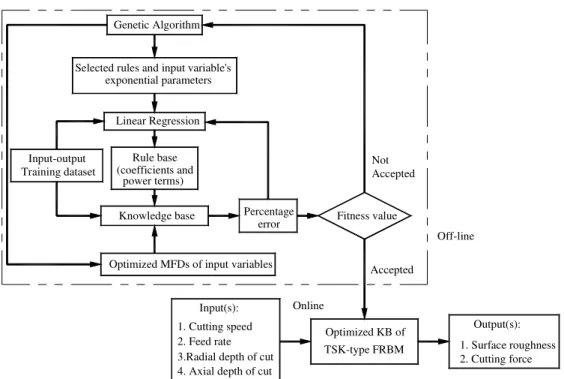
The main objective of constructing FRBM of a physical process is to design its optimum KB based on the measured example data. The KB of FRBM consists of rule base (RB) and fuzzy sub sets (or MFDs), also called database. Several methods had been suggested by various researchers for fuzzy rule generation. In this connection, work of Takagi, and Sugeno (1985), Abdelnour et al. (1991), Wang and Mendel (1992) are worth mentioning. Moreover, gradient descent method (Nomura et al., 1992), reinforcement learning technique (Fukuda et al., 1995), neural networks (Nauck et al., 1993), evolutionary algorithm (Hwang and Thompson, 1994), etc. are well employed to construct RB. In the present work, a combined approach of multiple linear regression and GA (Nandi, 2006), so called genetic linear regression approach is adopted to construct the KB of FRBM with TSK-type FLR, as illustrated in Fig. 1.
Selected rules and input variable's
Optimized MFDs of input variables exponential parameters
Knowledge base Training dataset
Input-output
Genetic Algorithm
power terms) (coefficients and Linear Regression
Rule base
error Fitness value
TSK-type FRBM Optimized KB of Online
Off-line
Accepted Percentage
Accepted Not
4. Axial depth of cut 3.Radial depth of cut 1. Cutting speed 2. Feed rate
Input(s):
2. Cutting force 1. Surface roughness
Output(s):
Figure 1. Flow chart of Genetic Linear Regression approach for construction of TSK-type FRBM.
The structure of trapezoidal MFDs as considered here for the input variables is represented in Fig. 2. Two parameters, b and d are needed to describe the (semi) trapezoidal MFDs. The scaling factors (MaxV – MinV) of all input variables are kept as same during optimization of MFDs in constructing each FRBMs for surface roughness and cutting force.
The optimal values of rule-consequent coefficients and power terms are obtained using genetic linear regression approach and simultaneous optimisation of input variable’s MFDs using GA, as presented in Fig. 1. The optimum values of power terms of rule consequent functions (p1, p2, p3 and p4, according to Eq. (2)) and the parameters related to MFDs (b and d, according to Fig. 2) are determined using GA, while the rule-consequent coefficient (a1, a2, a3 and a4 according to Eq. (2)) are determined using multiple linear regression method in the framework of genetic linear regression approach. As the performance of a GA depends on the GA-parameters, the optimal choices of GA-parameters (namely population size, crossover probability and mutation probability) are fixed through a parametric study (Nandi, 2006) in order to achieve good results.
d b
0.0 1.0
(MaxV-MinV)-b
Membership value
Input variable
L H
MinV MaxV
Figure 2. Structure of semi-trapezoidal MFDs with two fuzzy subsets.
Linear Regression Method with TSK-Type Fuzzy Model (Nandi and Klawonn, 2004)
A general expression of linear regression system with TSK-type fuzzy model is derived here to determine the coefficients of RCFs in
GLR approach. Equation (1) may be rewritten by denoting
(
)
∏ =
=
n 1 v
ηr x1,...,n
µv for simplicity, in the following form:
(
x1,...x n)
FY =
(
)
(
)
(
)
(
)
∑
=
+ + +
∑
= =
R l
1 r
ηr
x1,...,n f rk ark ... x1,...,n f r2 ar2 x1,..,n f r1 ar1 R l
1 r
ηr
(
)
(
)
(
)
(
)
(
)
(
)
(
)
(
)
ηRl
...
η2 η1
x1,.,n fRkl aRkl .. x1,.,n fR1l aR1l
ηRl
...
x1,.,n f 2k a2k .. x1,..,n f tr
t j atr
t j ... x1,..,n f tr1 atr1
η
tr
.... ... ... x1,.,n f1k a1k ... x1,.,n f11 a11
η1
+ + +
+ +
+
+
+ + +
+ +
+ +
+
=
Let us assume we have a set of input-output tuple (D) of S number of sample data where the output y( )i is assigned to the input
(
x i( ) ( )
1 ,x i2 ,... ,x s( )
n)
.( )
( ) ( )
(
)
(
( )
( ) ( )
)
(
( )
( ) ( )
)
{
x 11 ,....,x 1n,y 1 ,x 21 ,...,x 2n ,y 2 ...x s1 ,....,x sn,y s}
D=Now, the total quadratic error that is caused by the TSK-type FRBM with respect to the given data set is
(
)
(
)
s 2
(1) (1) (1) (1)
n
1 2
l 1
E f x ,x ,....x y
=
In order to minimise E, we have to choose the following parameters appropriately:
(
) (
)
(
)
{
a 11,...., a 1k , a 21,... a 2k ,..., a R1 ,...., a Rk}
,where the parameter arj indicates the jth coefficient of the output function of rth rule.
To determine the above parameters, we take the partial derivatives of E with respect to each parameter (arj) and make them be zero, i.e.,
0 a E r j = ∂ ∂
, where j=
{
1,2,....,k}
and r={
1,2,...,R}
Now, we obtain the partial derivation of E with respect to the parameter atrt j,
( )
( )
(
)
( )
(
)
(
( )
( )
)
∑ = ∂ ∂ ⋅ − ⋅ = ∂ ∂ S 1l atrt j
x ln ,..., x l1 f y l x ln ,..., x l1 f 2 atrt j
E × ∑ = − ∑ = ∑ = + + ⋅ = S 1 l y l R l 1 r ηr R l 1 r
xl1,..,n f rk ark ... x l1,..,n f r1 a r1 ηr 2 ∑ = ⋅ Rl 1 r ηr
xl1,..,n f trt j
η tr .
( )
(
)
(
)
( )
(
)
(
)
∑ = ∑ = ∑= + + ∑ = ∑ = ∑= = 2 Rl 1 r ηrxl1,..,n f trt j η tr S 1 l Rl 1
r arkfrkxl1,..,n ηr ... ... ... ... 2 Rl 1 r ηr
xl1,..,n f trt j S 1 l Rl 1 r η tr xl1,..,n fr1 ar1 ηr 2 0 R l 1 r ηr
x l1,..,n f t rt j S 1 l η t r y l 2 = ∑ = ∑ = ⋅
− , (4)
Thus, Eq. (3) provides the following system of linear equations from which we can compute the coefficients
(
) (
) (
)
{
a 11,....,a 1k, a 21,...a 2k,..., a R1 ,....,a Rk}
:( )
( )
( )
( )
( )
xl1,..,n n1 v
µtrv xl1,..,n
f trt j
xl1,..,n f rj S
1
l R l 2
1 r
n
1 v
xl1,..,n µrv n
1 v
xl1,..,n µrv R 1 r K 1 j arj ∏ = × × ∑ = ∑ = ∏= ∏ = ∑ = ∑ =
(
)
(
)
f t rt j(
x l1,..,n)
S1
l R l
1 r
n
1
v x l1,..,n µrv n
1 v
x l1,..,n µt rv y l ∑ = ∑ = ∏= ∏ =
= (5)
In matrix form, Eq. (5) will be written as:
= β . . . . . β β a . . . . . a a . α . . . . . α α . . . . . . . . . . . . . . . . . . . . . . . . . . . . . . . . . . . . . . . . α . . . . . α α α . . . . . α α r K r 2 r 1 r K r 2 r 1 r KK r K2 r K1 r 2K r 22 r 21 r 1K r 12 r 11 (6)
where α f
(
x,x ..,x) (
f x1l,xl2..,xln)
S 1 l r t l n l 2 l 1 r j r tj=∑= ;β y f
r t S 1 l l r t= ∑
= .
Thus Eq. (5) provides solutions of the function coefficients (arj) of the TSK-type fuzzy rule consequents for given values of the
input variable’s exponential terms.
Experimentation
For modelling cutting force in milling, modified AISI P20 tool steel is considered as the work piece material (Abou-El-Hossein et al., 2007). It is a chromium-molybdenum alloyed which is considered as high speed steel. AISI P20 defers from normal P20 steel by containing 0.015% Sulphur, because of better machinability and more uniform hardness in all dimension. Its tensile strength is 1044 MPa and its hardness range is 280 HB to 320 HB. The cutting tool used in this study is a 00 lead-positive end milling cutter of 31.75 mm diameter and equipped with two square inserts whose all four edges can be used for cutting. Here, one insert per one experiment is mounted on the cutter. The inserts have the following specification: square shape, back rake angle of 00, clearance angle of 110, nose radius of 0.794 mm and without any chip breaker. These carbide inserts are KC735M which have a single layer of TiN. The coating is accomplished using PVD techniques to a maximum of 0.004 mm thickness. Experiments are performed in random with different cutting conditions and using a standard coolant to find the cutting force. Each experiment is stopped after 85 mm cutting length. Fc is measured with the aid of a piezoelectric cutting force dynamometer provided by Kistler. Each experiment is repeated three times using a new cutting edge every time and the average of these values is considered.
end mill VC2SBR0300, diameter 6 mm is used. Effective Sr is measured with a Taylor–Hobson form Taylsurf series 2 profile rugosimeter in every experiment conducted with different cutting conditions.
Now, the data collected based on experimentation are analyzed in the following sub-section to reveal the preliminary information underlying in the relationship between input-output variables. This information is used in the GLR approach to construct the KB of FRBMs.
Experimental Data Analysis
Surface roughness
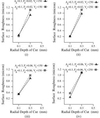
In order to understand the relationship of surface roughness with cutting parameters (feed rate, radial depth of cut, axial depth of cut and cutting speed), it is essential to analyse the variation of surface roughness with respect to each of the individual cutting parameter as well as when more than one parameter are changing simultaneously. After analysing the experimental data, as shown in Figs. 3(i)-(iv) which describe the variation of surface roughness with feed rate, the following points are revealed:
i)Surface roughness is deteriorated with increasing feed rate at a) any value of Ad and Vc but lower value of Rd (0.1 mm) b) lower value of Ad (0.1 mm) but higher value of Vc and
Rd (250 m/min and 0.1 mm, respectively), Fig. 3(iv) ii) Surface roughness improves with increase in feed rate at
a) any value of Ad, lower value of Vc (150 m/min) and higher value of Rd (0.3 mm), according to Fig. 3(iii) b) higher values of Ad (0.3 mm), Vc (250 m/min) and Rd
(0.3 mm), according to Fig. 3(iv)
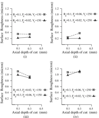
Figures 4(i)-(iv) describe the variation of surface roughness with respect to radial depth of cut. After analysing the data as shown in Figs. 4(i)-(iv), it has been revealed that surface roughness get worse by increasing the value of Rd at any values of axial depth of cut, feed rate and cutting speed, and the rate deterioration (considerably high) is almost the same for all values of Ad, Fd and Vc.
The variations of surface roughness with respect to axial depth of cut are illustrated in Figs. 5(i)-(iv). Analysis of data as presented in Figs. 5(i)-(iv) implies the following points:
i) Surface roughness is deteriorated (in different rates) with increasing axial depth of cut at
a. lower value of Rd (0.1), any values of Fd and Vc, Figs. 5(i)-(ii)
b. higher values of Rd (0.3) and Vc (250), and lower value of Fd (0.02), Fig. 5(iv)
ii) Surface roughness is improved with increasing axial depth of cut only at
a. higher value of Rd (0.3), any value of Fd and lower value of Vc (150), Fig. 5(iii)
After analysing the data as shown in Figs. 6(i)-(iv), which describe the variation of surface roughness with cutting speed, the following points are revealed:
i) Surface roughness is deteriorated with increasing cutting speed at a. any value of Ad, higher value of Rd (0.3) and any value
of Fd, Fig. 6(iv)
b. higher value of Ad (0.3), lower value of Rd (0.1) and higher value of Fd (0.06), Fig. 6(ii)
ii) Surface roughness is improved with increasing cutting speed at a. lower value of Ad (0.1), lower value of Rd (0.1) and any
value of Fd, Figs. 6(i), (ii) and (iii).
From the above analyses, it is stated that change in radial depth of cut influences much on surface roughness than other cutting parameters, namely axial depth of cut, cutting velocity and feed rate.
A =0.1, R =0.1, V =150 A =0.3, R =0.1, V =150
Feed (mm/rev) (i) 0.06 S u rf ac e R o u g h n es s (m ic ro n ) 0.2 0.4 0.6 0.8 0.02 d d d d 1.0 1.2
A =0.1, R =0.1, V =250
S u rf ac e R o u g h n es s (m ic ro n ) c 0.1 c 0.2 0.6 0.4 0.8 1.0 1.2
A =0.3, R =0.1, V =250c
Feed (mm/rev) c 0.02 (ii) 0.06 d d d d 0.1
Feed (mm/rev) A =0.3, R =0.3, V =150 A =0.1, R =0.3, V =150
S u rf ac e R o u g h n es s (m ic ro n ) 0.02 0.2 0.4 0.6 0.8 d d (iii) 0.06 d d c c 1.0 1.2 0.1 0.06 (iv) Feed (mm/rev) A =0.3, R =0.3, V =250
A =0.1, R =0.3, V =250
S u rf ac e R o u g h n es s (m ic ro n ) 1.2 1.0 0.8 0.6 0.4 0.2 0.02 d d d d c 0.1 c
Figure 3. Variation of surface roughness with feed rate.
A =0.1, F =0.02, V =150
0.3
Radial Depth of Cut (mm)
A =0.3, F =0.02, V =150
0.4 Su rf ac e R o u g h n es s (m ic ro n ) 0.2 (i) 0.1 1.2 0.8 0.6 1.0 d d d d Su rf ac e R o u g h n es s (m ic ro n ) d
A =0.1, F =0.02, V =250
Radial Depth of Cut (mm)
A =0.3, F =0.02, V =250d
0.4 Su rf ac e R o u g h n es s (m ic ro n ) 0.5 0.2 c c 1.2 0.8 0.6 1.0 (ii)
0.1 0.3 0.5 c d
d c
0.5
Radial Depth of Cut (mm)
0.4
0.2
0.1
(iii)
0.3 A =0.1, F =0.06, V =150
A =0.3, F =0.06, V =150 1.2 0.8 0.6 1.0 d d d c d c
A =0.3, F =0.06, V =250
0.3
Radial Depth of Cut (mm)
A =0.1, F =0.06, V =250
0.2 Su rf ac e R o u g h n es s (m ic ro n ) 0.1 (iv) 1.0 0.6 0.8 0.4 1.2 d d d d 0.5 c c
R =0.1, F =0.06, V =150
R =0.1, F =0.02, V =150
0.3
Axial depth of cut (mm) d d S u rf ac e R o u g h n es s (m ic ro n ) 1.0 0.2 0.6 0.4 0.8 0.1 (i) d d 1.2
R =0.1, F =0.06, V =250
R =0.1, F =0.02, V =250
Axial depth of cut (mm) c S u rf ac e R o u g h n es s (m ic ro n ) 1.0 0.5 c 0.2 0.6 0.4 0.8 1.2 d d c (ii) 0.1 0.3
d d c
0.5
0.5 Axial depth of cut (mm)
S u rf ac e R o u g h n es s (m ic ro n ) 1.0
R =0.3, F =0.06, V =150 R =0.3, F =0.02, V =150
0.2 0.1 0.6 0.4 0.8 d d (iii) 0.3 d d c c 1.2
R =0.3, F =0.06, V =250
R =0.3, F =0.02, V =250
Axial depth of cut (mm) 0.3 1.2 S u rf ac e R o u g h n es s (m ic ro n ) (iv) 1.0 0.6 0.8 0.2
0.4 d d
0.1 d d
c
0.5 c
Figure 5. Variation of surface roughness with axial depth of cut.
A =0.1, R =0.1, F =0.02
A =0.3, R =0.1, F =0.02
300
Cutting Speed (m/min)
S u rf ac e R o u g h n es s (m ic ro n ) 0.8 0.6 0.4 0.2 100 (i) d d d d 1.2 1.0
A =0.1, R =0.1, F =0.06
S u rf ac e R o u g h n es s (m ic ro n ) 500 d d 0.2 0.6 0.4 0.8 1.2 1.0
A =0.3, R =0.1, F =0.06
Cutting Speed (m/min)
100 (ii) 300 d d d d d d 500
A =0.3, R =0.3, F =0.02
A =0.1, R =0.3, F =0.02
Cutting Speed (m/min)
S u rf a ce R o u g h n e ss ( m ic ro n ) 100 0.2 0.8 0.6 0.4 d d 300 (iii) d d d d 1.2 1.0 500 (iv)
Cutting Speed (m/min)
300 A =0.1, R =0.3, F =0.06
A =0.3, R =0.3, F =0.06 1.2 S u rf ac e R o u g h n es s (m ic ro n ) 0.2 0.4 0.6 0.8 1.0 100 d d d d 500 d d
Figure 6. Variation of surface roughness with cutting speed.
Cutting Force
Like surface roughness, the influences of different cutting parameters (Fd, Ad, Rd and Vc) on cutting force generated during milling operation are illustrated in graphical manner based on
experimental data. This underlying information in the cutting force relation with cutting parameters extracted from experimental data is later utilized during learning of FRBM for constructing cutting force model.
Figures 7(i)-(iii) show the graphs representing the variation of cutting force with axial depth of cut. It is observed that cutting force increases with increasing axial depth of cut at almost equal rate at any values of Vc, Fd and Rd. Again it is observed in Fig. 7(iii) that, when cutting velocity is decreased, the amount of cutting force value is comparatively higher for the constant values of Fd and Rd.
Figures 8(i)-(iii) represent the variation cutting force with feed rate. It is found that cutting force increases with increase in feed rate for any values of Vc, Ad and Rd, but the increasing rate varies in different cases. Again in Fig. 8(i), when Ad changes the value from 1 mm to 2 mm, with increase in feed rate, the cutting force increases but it starts from a high value as well as with higher rate.
In Figs. 9(i)-(ii), the graphs are drawn showing the variation of cutting force with radial depth of cut. It is observed that cutting force increases with increase in radial depth of cut. It is observed that, if the value of Ad changes from 1 mm to 2 mm (Fig. 9(i)) and Vc changes value from 180 m/min to 100 m/min (Fig. 9(ii)), with increase in Rd, the cutting force value becomes high and it increases with almost equal rate.
In Figs. 10(i)-(iii), the curves are drawn representing the variation of cutting force with cutting speed. Here it is observed that with increase in cutting speed, the cutting force decreases for any values of Fd, Ad and Rd, i.e. proportionally inverse. For a given cutting speed, the cutting force value becomes high if Rd changes from 2 mm to 5 mm and Ad changes from 1 mm to 2 mm, as shown in Fig. 10(i) and Fig. 10(ii), respectively.
From the above analysis of experimental data, it is clearly observed that the outputs (surface roughness and cutting force) in milling are not linearly related with the cutting parameters and ambiguity is involved when more than one cutting parameters vary simultaneously.
V =140, F =0.15, R =2
Axial Depth of Cut (mm)
1 C u tt in g F o rc e ( N ) 300 200 100 400
V =180, F =0.15, R =3.5 V =100, F =0.15, R =3.5
Axial Depth of Cut (mm)
Axial Depth of Cut (mm)
(i)
2 3 4
(ii)
1 2 3 4
1
V =140, F =0.1, R =3.5
300 C u tt in g F o rc e ( N ) 100 200 400 300 C u tt in g F o rc e ( N ) 100 200 400 (iii)
2 3 4
c d d c
d d
d
c d d
c d
V =140, A =1, R =3.5 V =140, A =2, R =3.5
Feed (mm/rev.) 0.1 C u tt in g F o rc e ( N ) 100 400 200 300
V =140, A =1.5, R =5
Feed (mm/rev.)
V =100, A =1.5, R =3.5
Feed (mm/rev.) 0.1 C u tt in g F o rc e ( N ) (i)
0.2 0.3 0.4 100 400 300 200 C u tt in g F o rc e ( N ) (ii)
0.2 0.3 0.4
100 400 300 200 0.4 (iii) 0.1 0.2 0.3
c d d
c d d
c d d
c d d
Figure 8. Variation of cutting force with feed rate.
C u tt in g F o rc e ( N ) 300 300 C u tt in g F o rc e ( N )
Radial Depth of Cut (mm) V =140, F =0.15, A =1
Radial Depth of Cut (mm) 1
200
100
(i)
3 5 7
V =180, F =0.15, A =1.5
1 100 200
(ii)
3 5 7
V =140, F =0.15, A =2 400
V =100, F =0.15, A =1.5 400
c d d
c d d
c d d
c d d
Figure 9. Variation of cutting force with radial depth of cut.
C u tt in g F o rc e ( N )
Cutting Speed (m/min)
Cutting Speed (m/min) Cutting Speed (m/min)
(i) (ii) (iii) 200 C u tt in g F o rc e ( N ) d d d
F =0.15, A =1.5, R =2
100
50 150 200
100 200
F =0.15, A =1, R =3.5
50 d
100 150 d d F =0.15, A =2, R =3.5
100
200 d d d
F =0.15, A =1.5, R =5d d
300 400 d 300 400 C u tt in g F o rc e ( N ) 150
F =0.1, A =1.5, R =3.5
50 100
d d d
100 200
200 300
400
Figure 10. Variation of cutting force with cutting speed.
Mathematical Model
The mathematical model between cutting parameters (cutting velocity, feed rate, axial depth of cut and radial depth of cut) and the cutting force in milling operation (with workpiece material of AISI P20) was derived by using Box-Behnken design (one type of RSM) and it is defined by:
d d d d d d d c 2 d 2 d 2 d 2 c d d d c c R 14.05A R 33.33F A 600F R 0.0417V 2.02R 48.15A 307.67F 0.0089V 2.57R 166.07A 292.30F 3.09V 330.66 F + + + − + + − + + − + − = (7)
The regression model of surface roughness with cutting parameters for (climb) milling (with workpiece material of W-Nr) is derived by Vivancos et al. (2004), as follows:
c V d 0.0057915R d F d 17.0406R 2 d 14.6044R c V d A 0.00672575 c V 0.00250345 d 3.4081F d 2.49037R d 1.34515A 0.683042 r S + − + + − + − − = (8)
Training Data and Fitness Evaluation of GA
Training data
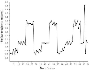
In order to determine the rule consequent function coefficients and power terms of a TSK-type FRBM, a huge number of example data are required. In the present study, 81 numbers of data (Fig. 11 and Fig. 12 related to cutting force and surface roughness, respectively) are considered for constructing KB of FRBMs. These data are obtained through real experimentation as well as based on empirical correlation models (as stated in the section “Mathematical Model”). However, those empirical models are not accurate. Hence, the results obtained using the empirical models do not follow the real characteristics of the relationships among input-output variables in milling process. For this reason, it is required to modify the data obtained using mathematical models to suit the process input-output relationship as discussed in experimental data analysis (in sub-section “Experimental Data Analysis”).
100 50 250 200 150 400 350 300 10
5 15 20 25 30 500
450
40
35 45 50 55 60 65 70 75 80
C u tt in g f o rc e ( N )
No of cases
N o of cases 40
Su
rf
a
ce
r
o
u
g
h
n
es
s
(
m
ic
ro
n
)
0.7
0.1 5 0.4 0.3 0.2 0.5 0.6
25 15
1 0 2 0 3 0 35 1.3
1.0
0.8 0.9 1.1 1.2 1.6 1.4 1.5
55
45 50 60 6 5 70 7 5 80 8 5 90
Figure 12. Training data: Surface roughness.
Fitness Evaluation of GA
During the iteration process of genetic algorithm, the GA population (individuals/chromosomes) having lower fitness value (for error minimization) is chosen in order to reproduce the child chromosomes in the next iteration using the three GA- operators, namely selection, cross-over and mutation. On the other hand, to have a better reliability of FRBM, the performance of FRBM is to be uniform throughout the entire input space. To achieve such consistent result of an FRBM, in every region of the input space the errors of all training data samples that are considered to be uniformly distributed over the whole range of the input variable’s space should be equally important for minimization in finding a lower fitness value. Thus, the fitness value of a GA solution is estimated based on the percentage error (instead of simple error) of each training data sample. The error of each set of training data is the deviation of the result (surface roughness) of the FRBM from that of the desired one. Since the error may be positive or negative, absolute value of the error is considered in determining average percentage error as a fitness value of GA-solution.
For cutting force, the fitness value of GA-solution during model construction is calculated in the same way as discussed above for surface roughness.
TSK-Type FRBM for Milling Process
In order to develop a suitable model for milling operation in the present work, four input process variables (cutting speed, feed rate, axial depth of cut and radial depth of cut) are considered. For each of the output variables (cutting force and surface roughness), the model is constructed based on the training data as depicted in Fig. 11, and Fig. 12, respectively. Each of the four input variables are considered to have semi-trapezoidal MFDs with two different linguistic values (L and H) (as shown in Fig. 2) and the corresponding scaling factors are 80, 0.1, 1.0 and 3.0, respectively, for all the TSK-type FRBMs corresponding to different outputs. Since each input variable has two linguistic terms within its range, there could be a maximum of
16 2 2 2
2× × × = rules in the RB of FRBM.
Model of Cutting Force
In order to develop a FRBM for cutting force in milling process, the structure of rule consequent function (as shown in Eq. (9)) considered here has four coefficients and four power terms. Thus the
RB, with a maximum of 16 rules in the rule premise, would have a total of 64 (16x4) coefficients and 64 power terms.
A GA-string of 720-bits long is considered for finding the RCFs parameters using GLR approach as well as optimization of MFDs of input variables. First 80 bits (10 bits for each variable) of the GA-string carry information of the eight continuous variables (two variables related to MFDs, b and d for each of the four inputs). The remaining 640 bits (10 bits for each variable) are used to obtain the values of 64 power terms. It is noted that during optimization of MFDs of input variables, the scaling factors (length of input range) of all input variables are not changed.
During GA-based optimization, the parameters related to MFDs – b1 and d1 (for cutting speed); b2 and d2 (for feed rate); b3 and d3 (axial depth of cut) and b4 and d4 (radial depth of cut), as shown in Fig. 2, are varied in the range of {(20, 60) and (0, 20)}; {(0.02, 0.05) and (0, 0.02)}; {(0.2, 0.8) and (0, 0.2)} and {(1, 2) and (0, 1)}, respectively. The values of power terms lie in the range of 0.0 to 3.0. The fitness values of GA solution are calculated using the procedure as discussed in sub-section “Fitness Evaluation of GA”. The optimal choices of GA-parameters (namely population size, crossover probability and mutation probability) are fixed through a parametric study in order to achieve good results.
After a parametric study of GA, the following GA parameters are selected for the best optimization during training of FRBM for cutting force prediction:
P = 100; Cp = 0.87; Mp = 0.011; Ng = 125.
4 3 2
1 p
d 4 p d 3 p d 2 p c
1V cF cA cR
c
Fc= + + + (9)
The optimized data base and rule base of FRBM for cutting force in milling obtained using Eq. (9) are shown in Fig. 13 and Table 1, respectively.
0.1
Cutting speed (m/min)
100 0.0 3.0
0.0 160
140 180
L H
3.0
Feed rate (mm/rev)
0.15
0.13 0.2
L H
2
Radial depth of cut (mm) Axial depth of cut (mm)
1 0.0 3.0
1.6 L
2 1.8
0.0 H
3.0
4 3 L
5 H
Figure 13. Optimized semi-trapezoidal MFDs of TSK-type FRBM for cutting force.
Model of Surface Roughness
(10 bits for each variable) are used to obtain the values of 64 power terms. It is noted that during optimization of MFDs of input variables, the scaling factors are not changed.
During GA-based optimization, the parameters related to MFDs – b1 and d1 (for cutting speed), b2 and d2 (for feed rate), b3 and d3 (for axial depth of cut), and b4 and d4 (for radial depth of cut), as shown in Fig. 2, are varied in the range of {(55.359, 105.359) and (0, 55.359)}, {(0.012, 0.052) and (0, 0.012)}, {(0.111, 0.211) and (0, 0.111)}, and {(0.111, 0.211) and (0, 0.111)}, respectively. In this case, the values of power terms are kept in the range of 0.0 to 2.0. The fitness values of GA solution are calculated using the same procedure as used in case of cutting force. After a parametric study
of GA, the following GA parameters are selected for best optimization during tuning of FRBM used for power prediction in milling:
P = 50; Cp = 0.98; Mp = 0.011; Ng = 125. 4 3
2
1 c f c A c R
V c
Sr = 1 cp + 2 dp + 3 dp + 4 pd (10) The optimized data base and rule base of the TSK-type FRBM for surface roughness obtained using Eq. (10) are shown in Fig. 14 and Table 2, respectively.
Table 1. Values of coefficients and power terms of TSK-type rules in optimized rule base of FRBM cutting force [(a) coefficient, (b) power terms].
(a) Coefficient
Rule No. Rule Antecedent Cutting Force
Vc Fd Ad Rd C1 C2 C3 C4
1 L L L L -0.258446 -454.6900 -20.94110 567.5480
2 L L L H 0.502033 -4586.570 21.87050 36.92860
3 L L H L -0.000921 565305000 -420648.0 7.543430
4 L L H H 0.042156 -16225.20 385.0280 -48.26390
5 L H L L -0.322918 4358.690 195.8770 1.738540
6 L H L H -11.65450 1961.360 13059.10 2262.630
7 L H H L 0.005987 1565.370 -113.280 11.31310
8 L H H H -10.20730 2541.820 1671170 -341836.0
9 H L L L -0.001152 964.6000 45.1810 81.62920
10 H L L H 0.000432 -1100.050 61.04240 -2.226270
11 H L H L -5.284520 -26908300 15328.60 20.63840
12 H L H H 279.5600 -1001790 568.4150 475.0060
13 H H L L -1.440340 2516.390 134.7630 209.5880
14 H H L H -2.696420 2835.470 22.03080 38286.10
15 H H H L 0.043724 1538.670 -702.4380 560.9770
16 H H H H -0.067508 3940.300 -59498.00 19939.90
(b) Power terms
Rule No. Rule Antecedent Cutting Force
Vc Fd Ad Rd P1 P2 P3 P4
1 L L L L 1.23460 0.03225 0.55718 0.13489
2 L L L H 1.39883 0.60410 0.76832 1.92962
3 L L H L 2.74194 2.98240 0.48387 1.87097
4 L L H H 1.90909 2.38710 2.23460 2.30205
5 L H L L 1.23754 2.34604 0.50146 2.81232
6 L H L H 1.91789 2.10264 0.17008 2.10557
7 L H H L 2.07038 0.38709 2.49853 1.87390
8 L H H H 1.24633 1.69795 1.48387 1.62463
9 H L L L 2.31672 0.87096 1.71261 0.28739
10 H L L H 2.14370 1.42815 2.24633 1.78299
11 H L H L 1.61584 2.89443 1.91202 0.79472
12 H L H H 0.53958 2.19062 1.16716 0.24633
13 H H L L 1.04985 2.11144 0.82991 0.27272
14 H H L H 2.66276 1.60411 1.85337 2.65103
15 H H H L 2.24047 1.10850 2.98240 0.17008
0.008 119.641
0.0 1.0
Cutting speed (m/min)
169.641 225 280.359
L H
0.048
Feed rate (mm/rev)
0.06 0.072
L H
Axial depth of cut (mm)
0.039 0.139 0.25 0.361
L H
0.361
Radial depth of cut (mm)
0.139
0.039 0.25
L H
0.0 1.0
0.0 1.0
0.0 1.0
Figure 14. Optimized semi-trapezoidal MFDs of TSK-type FRBM for surface roughness.
Table 2. Values of coefficients and power terms of TSK-type rules in optimized rule base of FRBM: Surface roughness [(a) coefficient, (b) power terms].
(a) Coefficient
Rule No. Rule Antecedent Surface Roughness
Vc Fd Ad Rd C1 C2 C3 C4
1 L L L L 0.027802 51.07870 0.054873 -1.363000
2 L L L H 0.000003 -0.369016 0.052852 10.89830
3 L L H L 0.056442 6.056330 1.163300 -80.00000
4 L L H H -0.118721 0.353802 -0.926731 4.708700
5 L H L L 0.011655 0.697784 -0.221793 2.202150
6 L H L H -0.000188 83.26960 -0.311935 7.627010
7 L H H L -0.002009 -116.8980 4.830190 0.000000
8 L H H H -2.695120 -155.1670 360.7270 6.013470
9 H L L L -0.018567 0.763311 0.333107 0.748771
10 H L L H -0.000006 -1.843820 0.154931 9.455500
11 H L H L -0.000018 1.928620 0.427665 0.082161
12 H L H H -0.000003 -15.44880 -0.035930 8.419270
13 H H L L 0.020635 -8.261550 0.635194 27.01110
14 H H L H -0.000007 -2.869020 -0.101510 5.972600
15 H H H L 0.687483 -27.87730 3.052320 -8.210860
16 H H H H -0.000158 -7.426170 -88.00250 17.59480
(b) Power terms
Rule No. Rule Antecedent Surface Roughness
Vc Fd Ad Rd P1 P2 P3 P4
1 L L L L 0.47702 1.94526 1.91398 1.16520
2 L L L H 2.00000 0.70576 0.25219 2.00000
3 L L H L 0.44379 1.35679 0.18377 1.81036
4 L L H H 0.38123 0.37536 0.45747 0.62952
5 L H L L 0.67644 0.94428 0.48875 1.83773
6 L H L H 1.46628 1.74976 0.18377 1.79277
7 L H H L 0.99120 1.83187 1.08504 0.59628
8 L H H H 0.37145 0.42619 1.43109 1.91007
9 H L L L 0.36950 0.93841 1.99413 0.37536
10 H L L H 1.62463 1.32356 0.48289 1.83773
11 H L H L 1.17693 1.43109 0.84262 0.18181
12 H L H H 1.61877 1.97654 0.26197 1.63832
13 H H L L 0.09775 1.43891 1.99218 1.88856
14 H H L H 1.75171 0.81524 1.70674 1.18084
15 H H H L 0.17008 1.30010 0.75268 0.63734
Results and Discussions
Cutting force
The developed FRBM will be used for prediction cutting force and parameter optimization to achieve a desired objective in milling operation. In order to demonstrate the prediction capability of FRBM, both the results of FRBM and mathematical correlation model (available in the literature) are compared with the experimental data. For this comparative study, 22 numbers of cases are considered at random and the results of FRBM, mathematical model and experimentation for the 22 cases are enlisted in Table 3. In Table 3, Error I is the deviation (in percentage) of the result obtained using FRBM from that of the experimental value. Whereas, Error II is the percentage deviation of the result obtained using mathematical correlation model (Eq. (7), as shown in the section “Mathematical model”) from that of the experimental value.
In Table 3, it is observed that for almost all the cases, FRBM outperforms over the mathematical correlation model. For 11 cases (case no 1, 2, 7, 9, 10, 12, 14, 16, 17, 20 and 22), it is found that the results obtained by the FRBM are much better than the corresponding mathematical correlation results. Moreover, it is observed that RMS (root mean square) value (4.097) of Error I (evaluated in TSK-type FRBM model) is less than the RMS value (4.248) of Error-II (evaluated in mathematical model).
Thus, the developed FRBM may be adopted for prediction of cutting force to achieve a desired objective in drilling. The performance of FRBM may be improved by considering the
interaction effect(s) of the four cutting parameters in the rule consequent functions. But, in such cases, the computational complexity during model construction will be higher. For this reason, it is important to investigate the level of contribution(s) of the independent parameter’s interactions toward cutting force, which may be achieved using statistical approach such as analysis of variance (ANOVA).
Surface roughness
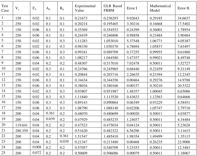
The developed FRBM for surface roughness will be used for prediction and parameter optimization to achieve a desired surface roughness in milling operation. The prediction capability of FRBM is verified by comparing the results of FRBM and mathematical correlation model with the experimental results. For this comparative study, 25 cases are considered at random and the results of FRBM, mathematical model and that of experimentation for the 25 cases are enlisted in Table 4. In Table 4, Error I is the deviation (in percentage) of the result obtained using FRBM from that of the experimental value. Whereas, Error II is the percentage deviation of the result obtained using mathematical model (Eq. (8), as shown in the section “Mathematical model”) from that of the experimental value.
In Table 4, it can be seen that in most of the cases, FRBM gives better results than mathematical correlation model, except in cases no. 5 and 9. Moreover, it is observed that RMS value (3.410) exhibited by the TSK-type FRBM model is less than that found by mathematical correlation model (RMS value = 11.65456173).
Table 3. Comparative results of FRBM and mathematical model: Cutting force.
Test
Case Vc Fd Ad Rd
Experimental Value
GLR Based
FRBM Error I
Mathematical Correlation Model
Error II
1 100 0.1 1.5 3.5 190 189.478 0.274736 191.1438 0.602000
2 100 0.15 1.5 2 210 206.895 1.478571 199.1439 5.169559
3 100 0.15 2 3.5 320 312.049 2.484687 323.7356 2.167398
4 100 0.15 1.5 5 315 328.413 4.258095 315.4374 0.138865
5 100 0.2 1.5 3.5 320 302.672 5.415000 312.8092 2.247125
6 140 0.1 1.5 2 100 99.9121 0.087900 98.54580 1.454200
7 140 0.1 1 3.5 110 117.244 6.585454 115.2308 4.755272
8 140 0.1 2 3.5 200 203.076 1.538000 203.1358 1.567900
9 140 0.1 1.5 5 210 209.779 0.105238 204.8358 2.459142
10 140 0.15 1 2 127.46 115.983 9.004393 121.3454 4.797250
11 140 0.15 2 2 210 203.237 3.220476 218.0254 3.821630
12 140 0.15 1.5 3.5 210 208.009 0.948095 208.7476 0.596345
13 140 0.15 1 5 225 205.522 8.656888 211.4099 10.040033
14 140 0.15 2 5 350 357.804 2.229714 350.5399 0.154264
15 140 0.2 1.5 2 200 210.038 5.019000 215.2117 7.605850
16 140 0.2 1 3.5 210 210.914 0.435238 206.8962 1.478000
17 140 0.2 2 3.5 360 366.947 1.929722 354.8012 1.444111
18 140 0.2 1.5 5 320 302.295 5.532812 331.5007 3.593968
19 180 0.1 1.5 3.5 130 130.565 0.434615 131.6278 1.252153
20 180 0.15 1.5 2 145 153.624 5.947586 144.6319 0.253844
21 180 0.15 1 3.5 140 139.679 0.229285 146.3146 8.510482
Table 4. Comparative results of FRBM and mathematical model: Surface roughness.
Test
Case Vc Fd Ad Rd
Experimental Value
GLR Based
FRBM Error I
Mathematical
Model Error II
1 150 0.02 0.1 0.1 0.21673 0.236293 9.02643 0.29185 34.6637
2 250 0.02 0.1 0.1 0.20214 0.195465 3.30216 0.16668 17.5402
3 150 0.06 0.1 0.1 0.35369 0.354553 0.24399 0.36001 1.78954
4 250 0.06 0.1 0.1 0.24439 0.246806 0.98858 0.23484 3.90484
5 150 0.02 0.1 0.3 1.11283 1.053010 5.37548 1.06771 4.05387
6 250 0.02 0.1 0.3 0.98330 1.030370 4.78694 1.05837 7.63497
7 150 0.06 0.1 0.3 0.99341 0.989709 0.37255 0.99955 0.61860
8 250 0.06 0.1 0.3 1.08217 1.044580 3.47357 0.99021 8.49748
9 200 0.04 0.2 0.2 0.48307 0.517010 7.02478 0.50011 3.52727
10 150 0.02 0.3 0.1 0.24766 0.245965 0.68440 0.22459 9.31149
11 250 0.02 0.3 0.1 0.20844 0.203716 2.26635 0.23394 12.2345
12 150 0.06 0.3 0.1 0.34434 0.344356 0.00464 0.29276 14.9788
13 250 0.06 0.3 0.1 0.38016 0.380166 0.00157 0.30210 20.5322
14 150 0.02 0.3 0.3 0.93807 0.951987 1.48357 1.00045 6.65086
15 250 0.02 0.3 0.3 1.11840 1.113520 0.43633 1.12563 0.64666
16 150 0.06 0.3 0.3 0.89143 0.890864 0.06349 0.93229 4.58451
17 250 0.06 0.3 0.3 1.08790 1.088140 0.02206 1.05747 2.79710
18 200 0.04 0.361 0.2 0.48070 0.480699 0.00020 0.50011 4.03877
19 200 0.04 0.039 0.2 0.47929 0.485235 1.24037 0.50011 4.34484
20 119.641 0.04 0.2 0.2 0.47523 0.475034 0.04124 0.50011 5.23628
21 280.359 0.04 0.2 0.2 0.51620 0.482322 6.56296 0.50011 3.11615
22 200 0.04 0.2 0.361 1.51547 1.485410 1.98354 1.49499 1.35115
23 200 0.04 0.2 0.039 0.21347 0.213480 0.00468 0.26235 22.9008
24 200 0.008 0.2 0.2 0.57057 0.540709 5.23353 0.50011 12.3483
25 200 0.072 0.2 0.2 0.50609 0.506086 0.00079 0.50011 1.18067
Likewise cutting force model, the performance of FRBM of surface roughness may be improved by considering the interaction effect(s) of the independent input parameters in the rule consequent functions. However, investigation on the level of contribution(s) of the independent parameter’s interactions is important.
Conclusion
In this work an attempt has been made to develop suitable TSK-type FRBMs for modelling of surface roughness and cutting force in milling operation.
In order to carry out these objectives, the present research work is carried out in three successive stages:
1. Experimentation and data analysis
2. Use of suitable techniques for constructing FRBM based on example data
3. Validation of FRBM
From experimental study, it is found that change in radial depth of cut influences much on surface roughness than other cutting parameters such as axial depth of cut, cutting velocity and feed rate. On the other hand, surface roughness and cutting force in milling are not linearly related to the cutting parameters and ambiguity happens by varying multiple cutting parameters simultaneously. For constructing the TSK-type FRBM, a combined approach of multiple linear regression method and genetic algorithm is utilized. The function coefficients are determined by linear regression whereas the optimized values of the exponential parameters are obtained by
using GA. In addition to that, the MFDs of input variables (cutting speed, feed rate, axial depth of cut and radial depth of cut) are simultaneously optimized in order to improve the performances of the FRBMs. After validation of each of the models corresponding to different outputs (surface roughness and cutting force) with the experimental data, it is suggested that both the FRBMs give satisfactory results showing excellent trade-off and practical implementation.
Acknowledgements
The author is thankful to DIT (Department of Information Technology), New Delhi, India for financial support of the grant-in-aid project (Ref No. 31(1)/2007-IEAD).
References
Abdelnour, G.M., Chang, C.H., Huang, H.H. and Cheung, J.Y., 1991, “Design of a Fuzzy Controller Using Input and Output Mapping Factors”,
IEEE Transactions on Systems, Man, and Cybernetics, Vol. 21, No. 5, pp. 952-960.
Abou-El-Hossein, K.A., Kadirgama, K., Hamdi, M. and Benyounis, K.Y., 2007, “Prediction of cutting force in end-milling operation of modified AISI P20 tool steel”, Journal of Materials Processing Technology, Vol. 182, No. 1-3, pp. 241-247.
Alauddin, M., E1 Baradie, M.A. and Hashmi, M.S.J., 1995, “Computer-aided analysis of a surface-roughness model for end milling”, Journal of Materials Processing Technology, Vol. 55, No. 2, pp. 123-127.
Armarego, E.J.A. and Brown, R.H., 1969, “The Machining of Metals”, Prentice-Hall, New Jersey.
Armarego, E.J.A., 1994, “Machining performance prediction for modern manufacturing”, Proceedings of the 7th International Conference on
Production and Precision Engineering and Fourth International Conference on High Technology (4th ICHT), Chiba, Japan, pp. 215-220.
Chang, C.C., 1992, “Mathematical modeling and analysis of the surfacetopography generated during end milling process”, Master Thesis, University of Maryland.
Chevrier, P., Tidu, A., Bolle, B., Cezard, P. and Tinnes, J.P., 2003, “Investigation of surface integrity in high speed end milling of a low alloyed steel”, International Journal of Machine Tools and Manufacture, Vol. 43, No. 11, pp. 1135-1142.
DeVor, R.E., Kline, W.A. and Zdeblick, W.J., 1980, “A mechanistic model for the force system in end milling with application to machining airframe structures”, Proceedings of the Eighth North American Manufacturing Research Conference, Rolla, pp. 297-303.
Dewes R.C. and Aspinwall, D.K., 1997, “A review of ultra high speed milling of hardened steels”, Journal of Materials Processing Technology, Vol. 69, No. 1-3, pp. 1-17.
Fukuda, T., Hasegawa, Y., Shimojima, K. and Saito, F., 1995, “Reinforcement Learning Method for Generating Fuzzy Controller”, Proceedings of the IEEE International Conference on Evolutionary Computation, pp. 273-278.
Ghani, J.A., Choudhury, I.A. and Hassan, H.H., 2004, “Application of Taguchi method in the optimization of end milling parameters”, Journal of Materials Processing Technology, Vol. 145, No. 1, pp. 84-92.
Hwang, W.R and Thompson, W.E., 1994, “Design of fuzzy logic controllers using genetic algorithms”. Proceedings of the Third IEEE International Conference on Fuzzy Systems (FUZZ-IEEE'94), Orlando, USA, pp. 1383-1388.
Kang, I.S., Kim, J.S., Kim, J.H., Kang, M.C. and Seo, Y.W., 2007, “A mechanistic model of cutting force in the micro end milling process”,
Journal of Materials Processing Technology, Vol. 187-188, pp. 250-255. Kline, W.A., DeVor, R.E. and Shareef, I.A., 1982, “The prediction of surface accuracy in end milling”, Transactions of ASME, Journal of Engineering for Industry, Vol. 104, pp. 272-278.
Koenigsberger, F. and Sabberwal, A.J.P., 1961, “An investigation of the cutting force pulsations during the milling process”, International Journal of Machine Tool Design and Research, Vol. 1, No. 1-2, pp. 15-33.
Kovacic, M., Balic, J. and Brezocnik, M., 2004, “Evolutionary approach for cutting forces prediction in milling”, Journal of Materials Processing Technology, Vol. 155-156, pp. 1647-1652.
Lee, H. U. and Cho, D. W., 2007, “Development of a reference cutting force model for rough milling feedrate scheduling using FEM analysis”,
International Journal of Machine Tools and Manufture, Vol. 47, No. 1, pp. 158-167.
Li, X.P., Nee, A.Y.C., Wong, Y.S. and Zheng, H.Q., 1999, “Theoretical modelling a simulation of milling forces”, Journal of Materials Processing Technology, Vol. 89-90, pp. 266-272.
Li, H.Z. and Li, X.P., 2002, “Milling force prediction using a dynamic shear length model”, International Journal of Machine Tools and Manufacture, Vol. 42, No. 2, pp. 277-286.
Li, H.Z., Zeng, H. and Chen, X.Q., 2006, “An experimental study of tool wear and cutting force variation in the end milling of Inconel 718 with coated carbide inserts”, Journal of Materials Processing Technology, Vol. 180, No. 1-3, pp. 296-304.
Montgomer, D.C., 2001, “Design, Analysis of Experiments”, 5th ed., John Wiley & Sons, pp. 427-500.
Nandi, A.K., 2006, “TSK-Type FLC using a combined LR and GA: surface roughness prediction in ultraprecision turning”, Journal of Materials Processing Technology, Vol. 178, No. 1-3, pp. 200-210.
Nandi, A.K. and Klawonn, F., 2004, “Detecting Ambiguity in RP using TSK models”, Proceedings of the IEEE International conference on Fuzzy Systems (FUZZ-IEEE 2004), Budapest, Hungary, pp. 221-226.
Nauck, D., Klawonn, F. and Kruse, R., 1993, “Combining Neural Networks and Fuzzy Controllers”. In E. -P. Klement, Slany W. eds. Fuzzy Logic in Artificial Intelligence, Springer, Berlin.
Nomura, H., Hayashi, I. and Wakami, N., 1992, “A learning method of fuzzy inference rules by descent method”, Proceedings of IEEE International Conference on Fuzzy Systems, San Diego, CA, USA, pp. 203-210.
Omar, O.E.E.K., El-Wardany, T., Ng, E. and Elbestawi, M.A., 2007, “An improved cutting force and surface topography prediction model in end milling”, International Journal of Machine Tools & Manufacture, Vol. 47, No. 7-8, pp. 1263-1275.
Sabberwal, A.J.P., 1960, “Chip section and cutting force during the end milling operation”, Annals of the CIRP, Vol. 10, No. 3, pp. 197-203.
Sugeno, M. and Kang, G.T., 1988, “Structure identification of fuzzy model”, Fuzzy Sets and Systems, Vol. 28, No. 1, pp. 15-33.
Sutherland, J.W. and DeVor, R.E., 1986, “Improved method for cutting force and surface error prediction in flexible end milling systems”,
Transactions of ASME, Journal of Engineering for Industry, Vol. 108, No. 4, pp. 269-279.
Takagi, T. and Sugeno, M., 1985, “Fuzzy identification of systems and its application to modeling and control”, IEEE Transaction on Systems, Man and Cybernetics, Vol. 15, No. 1, pp. 116-132.
Tsai, Y.H., Chen, J.C. and Lou, S.J., 1999, “An in-process surface recognition system based on neural networks in end milling cutting operations”, International Journal of Machine Tools and Manufacture, Vol. 39, No. 4, pp. 583-605.
Vivancos, J., Luis, C.J., Costa, L. and Ort´ız, J.A., 2004, “Optimal machining parameters selection in high speed milling of hardened steels for injection moulds”, Journal of Materials Processing Technology, Vol. 155-156, pp. 1505-1512.
Wang, L.X. and Mendel, J.M., 1992, “Generating Fuzzy Rules by Learning from Examples”, IEEE Transactions on Systems, Man, and Cybernetics, Vol. 22, No. 6, pp. 1414-1427.
Wang, S. M., Chiou, C.H. and Cheng, Y.M., 2004, “An improved dynamic cutting force model for end-milling process”, Journal of Materials Processing Technology, Vol. 148, No. 3, pp. 317-327.
Yoon, M.C. and Kim, Y.G., 2004, Cutting force modeling of endmilling operation, Journal of Materials Processing Technology, Vol. 155-156, pp. 1383-1389.
Yun, W.-S. and Cho, D.-W., 2000, “An improved method for the determination of 3D cutting force coefficients and runout parameters in end milling”, International Journal of Advanced Manufacturing Technology, Vol. 16, pp. 851-858.
Yun, W.-S. and Cho, D.-W., 2001, “Accurate 3-D cutting force prediction using cutting condition independent coefficients in end milling”,
International Journal of Machine Tools and Manufacture, Vol. 41, No. 4, pp. 463-478.
Zadeh, L.A., 1965, “Fuzzy Sets”, Information and Control, Vol. 8, pp. 338-353.

![Table 1. Values of coefficients and power terms of TSK-type rules in optimized rule base of FRBM cutting force [(a) coefficient, (b) power terms]](https://thumb-eu.123doks.com/thumbv2/123dok_br/18976201.455418/9.892.125.773.370.984/table-values-coefficients-power-terms-optimized-cutting-coefficient.webp)