NM-MRI for treatment evaluation of Parkinson’s Disease patients

Joana Micaelo Grilo

Bachelor of Science in Biomedical Engineering

NM-MRI for treatment evaluation of Parkinson’s

Disease patients

Dissertation submitted in partial fulfillment of the requirements for the degree of

Master of Science in Biomedical Engineering

Adviser: Rita G. Nunes, Assistant Professor,

Instituto Superior Técnico, University of Lisbon Co-adviser: Sofia Reimão, Neuroradiologist,

Faculty of Medicine, University of Lisbon and Hospital de Santa Maria,

Centro Hospitalar Lisboa Norte

Examination Committee

Chairperson: Doctor Carla Maria Quintão Pereira

NM-MRI for treatment evaluation of Parkinson’s Disease patients

Copyright © Joana Micaelo Grilo, Faculty of Sciences and Technology, NOVA University of Lisbon.

Acknowledgements

Foremost, I would like to express my sincere gratitude to my advisers Prof. Rita Nunes and Dr. Sofia Reimão for all the guidance, sympathy, knowledge and continuous support. I could not have imagined having better advisers. You gave me motivation when I needed it the most. Thank you for everything.

I would like to thank the Faculty of Sciences and Technology of NOVA University of Lisbon for providing me an immense knowledge.

I would also like to thank the Institute for Systems and Robotics of Instituto Superior Técnico and all the amazing people that I got to meet there for the wonderful welcome and inclusion. A special thanks to my lab partner and great friend Ana Fouto for all the help, the snack breaks much needed to regain energy and the reprehensible but at the same time kind words when I lost focus.

I would also like to thank my parents for providing me everything I needed and more, a great education, unconditional love, freedom and trust that I would do my best throughout these five years. Thank you to my beautiful sisters for the friendship and motivation. Also, a special thank to my boyfriend for always believing in me when I often doubted my abilities and for all the support and help.

A b s t r a c t

T1-weighted fast spin echo magnetic resonance imaging (MRI) sequences are able to depict neuromelanin (NM)-containing structures, such as the Substantia nigra (SN), as hyper-intense signal areas. NM-MRI can accurately discriminate Parkinson’s Disease (PD) patients from controls and could potentially be used to evaluate the effects of PD treatment - either surgery or medication. PD patients that are treated with Deep Brain Stimulation (DBS) can only undergo 1.5T MRI sequences with specific conditions that prevent the tissues surrounding the neurostimulators from overheating. However, NM-MRI sequences are usually not applied at 1.5T due to worse image quality. Nevertheless, it would be interesting to study how DBS and medication influence the NM signal as a path for a better understanding of the disease and to potentially evaluate the progression of PD after the surgical intervention.

Firstly in this work, a NM-MRI sequence was adapted for scanning patients with implanted DBS systems at 1.5T. To evaluate the performance of the sequence, images were taken on the same day with 1.5T and 3T MRI systems. The contrast ratio of both sequences was evaluated and SN areas were measured resorting to a semi-automatic segmentation algorithm. The assessment of these measurements revealed a good agreement between the developed sequence and the original 3T sequence.

A second study was carried out, in which SN areas of PDde novopatients were evaluated before and after two months of initiating pharmacological treatment. The median SN area tended to be increased after treatment, suggesting a potential increase of NM related to dopamine therapy.

In conclusion, this work presented the first 1.5T NM-MRI sequence that enables SN area measurement of patients with implanted neurostimulators, for further investigation of this method as a diagnostic tool for assessment of disease progression and to better understand clinical effects on NM-MRI and PD itself.

R e s u m o

A técnica de imagem por ressonância magnética (IRM) recorrendo a sequênciasfast spin echo permite distinguir estruturas relacionadas com Doença de Parkinson (DP), como a

Substantia nigra (SN), devido ao sinal hiper-intenso proveniente da neuromelanina (NM). Estas imagens discriminam pacientes com DP de controlos e podem potencialmente avaliar os efeitos da terapêutica - tanto medicação como cirurgia. Pacientes com DP que são tratados com estimulação profunda, para evitar o sobreaquecimento dos tecidos em contacto com os elétrodos durante exames subsequentes à cirurgia, apenas podem ser monitorizados a 1.5T. Apesar das imagens a 1.5T apresentarem pior qualidade, seria interessante estudar a influência da estimulação no sinal da NM, na medida em que poderia contribuir para a monitorização dos doentes após a cirurgia.

Neste trabalho, foi adaptada uma sequência sensível a NM para permitir a monitoriza-ção a 1.5T de doentes com neuroestimuladores implantados. Para avaliar o seu desempenho, foram efetuados exames a 3T e 1.5T no mesmo dia. O contraste das mesmas foi avaliado e utilizou-se uma ferramenta de segmentação semiautomática para medir as áreas da SN. As áreas medidas com a sequência desenvolvida e a sequência original a 3T mostraram uma boa concordância.

Adicionalmente, as áreas da SN de pacientes DP de novoforam medidas antes e após dois meses de iniciar a medicação. Verificou-se uma tendência de aumento da SN após tratamento, sugerindo um potencial aumento da neuromelanina relacionado com a terapia de dopamina.

Para concluir, este trabalho apresentou a primeira sequência de IRM sensível a neuro-melanina que permite medir as áreas da SN de pacientes de DP com neuroestimuladores implantados. Esta sequência pode vir a ser utilizada como uma ferramenta de avaliação da progressão da doença e contribuir para um melhor entendimento dos efeitos da terapêutica neste tipo de imagens assim como aprofundar os conhecimentos da DP.

C o nt e nt s

List of Figures xv

List of Tables xvii

Acronyms xix

1 Introduction 1

1.1 Motivation . . . 1

1.2 Aim of this work . . . 2

1.3 Thesis Outline . . . 2

2 Theoretical Principles and State of the Art 5 2.1 Magnetic Resonance Imaging . . . 5

2.1.1 Physical Fundamentals. . . 5

2.1.2 MR Pulse Sequences . . . 6

2.1.3 Generating image contrast. . . 8

2.1.4 Spatial Resolution and SNR . . . 9

2.2 Parkinson´s Disease . . . 10

2.2.1 Pathophysiology of PD. . . 10

2.2.2 Neuromelanin . . . 12

2.3 Deep Brain Stimulation . . . 13

2.3.1 Introduction to the technique . . . 13

2.3.2 Safety Concerns . . . 14

2.4 NM-MRI sequence . . . 16

2.5 Statistical Tests . . . 20

2.5.1 Non-parametric Tests . . . 20

2.5.2 Intraclass Correlation Coefficient . . . 20

2.5.3 Bland-Altman Method . . . 21

3 Validation of a 1.5T NM-MRI sequence 23 3.1 Materials and Methods. . . 23

3.1.1 Sample Description. . . 23

C O N T E N T S

3.1.2.1 Analysis of the acquisition parameters . . . 24

3.1.3 Imaging Analysis . . . 25

3.1.3.1 Segmentation method . . . 25

3.1.3.2 Similarity Analysis. . . 30

3.1.3.3 Image contrast Analysis . . . 30

3.1.4 Statistical Analysis . . . 32

3.2 Results. . . 33

3.3 Discussion . . . 39

4 Adaptation of the 1.5T NM-MRI sequence for DBS patients 43 4.1 Materials and Methods. . . 43

4.1.1 Sample Description. . . 43

4.1.2 Imaging Protocol . . . 44

4.1.2.1 Analysis of the acquisition parameters . . . 44

4.1.3 Imaging Analysis . . . 45

4.1.4 Statistical Analysis . . . 45

4.2 Results. . . 46

4.3 Discussion . . . 50

5 Imaging Study of therapeutic effects on PD patients 53 5.1 Review on the dopamine metabolism . . . 53

5.2 Materials and Methods. . . 55

5.2.1 Sample Description. . . 55

5.2.2 Imaging Protocol . . . 55

5.2.3 Imaging Analysis . . . 55

5.2.4 Statistical Analysis . . . 56

5.3 Results. . . 56

5.4 Discussion . . . 56

6 Conclusions and Future Work 59 6.1 Conclusions . . . 59

6.2 Suggestions for Future Work . . . 60

Bibliography 63

A Developed Interface 71

L i s t o f F i g u r e s

2.1 Representation of the protons in the absence of an external magnetic field. . 5

2.2 Representation of a Spin Echo Sequence.. . . 7

2.3 Representation of a Fast Spin Echo Sequence and corresponding K-space. . . 7

2.4 Representation of a Gradient Echo Sequence. . . 8

2.5 Influence of parameters TE and TR on the resulting weighted images. . . 9

2.6 Midbrain section of the mesencephalon. . . 11

2.7 Brain anatomy related with PD. . . 12

2.8 Midbrain sections showing the neuronal loss in a PD brain and a healthy subject brain. . . 13

2.9 Medtronic DBS System components. . . 14

2.10 Illustration of the STN electrical stimulation effects on PPT and SN. . . 14

2.11 The Medtronic 3389 Deep Brain Stimulation electrodes. . . 15

2.12 NM-sensitive and conventional MR images of the substantia nigra. . . 17

2.13 Correct slice orientation of a NM-sensitive MRI sequence. . . 17

2.14 Example of a Bland-Altman plot. . . 21

3.1 Axial sections at different levels of the midbrain showing the SN as a hyper intense signal area. . . 26

3.2 Selected axial middle slice for SN measurements before and after the application of the Gaussian blur filter.. . . 26

3.3 Representation of the 5x5 Gaussian blur colored image. . . 27

3.4 OsiriX segmentation tool interface that enables the definition of the segmenta-tion algorithm and respective parameters. . . 28

3.5 Illustration of the SN semi-automatic segmentation process. . . 29

3.6 Example of the application of a manual and semi-automatic segmentation of the SN. . . 29

3.7 Segmented regions after binarization and two available display options for visualizing the resulting overlap - with the Matlab application. . . 31

3.8 Example of a NM-MR image with two square ROIs in the SN and a circular reference ROI for CR calculation. . . 32

L i s t o f F i g u r e s

3.10 Box and whisker plot of DSC representing overlap between the segmented SN

areas and the manual ROI, for 1.5T and 3T. . . 35

3.11 Bland-Altman agreement plot of SN areas between the two different sequences

– 1.5T and 3T. . . 36

3.12 Dispersion of the SN CR at 1.5T and 3T, before and after the Gaussian blur

filter application. . . 37

4.1 Bland-Altman agreement plot of SN areas between the two different 1.5T

se-quences – general and optimized for DBS. . . 47

4.2 Dispersion of the SN CR after the Gaussian blur filter application, with the

1.5T NM-MRI sequences. . . 47

4.3 Axial sections at the level of the midbrain showing the SN area, taken with

three different NM-MRI sequences. . . 49

4.4 Axial section at the level of the upper midbrain with the right DBS electrode

visible in the slice. . . 52

5.1 Dopamine metabolism on a DAergic neuron. . . 54

5.2 Box and whisker plot of the SN areas estimated from the NM-MR images taken

before and after medication. . . 57

A.1 Developed interface in Matlab for the Dice Similarity Coefficient calculation

between two DICOMs containing segmented areas. . . 72

L i s t o f Ta b l e s

2.1 SAR and B1+RM S maximum values. . . 16

2.2 MRI protocols of several neuromelanin-sensitive MRI sequences. . . 19

3.1 ICC and Friedman test results (SN area and DSC) between repeated measures

at both field strengths. . . 38

4.1 ICC and Friedman test results (SN area) between repeated estimates for the

general and DBS 1.5T NM-MRI sequences. . . 48

4.2 SN areas of the same patient measured in three different NMMRI sequences

Ac r o ny m s

CI Confidence Intervals. CR Contrast Ratio.

DA Dopamine.

DBS Deep Brain Stimulation. DSC Dice Similarity Coefficient.

FA Flip Angle.

FID Free Induction Decay. FOV Field of View.

FSE Fast Spin Echo.

FWHM Full Width at Half Maximum.

GE Gradient Echo.

ICC Intraclass Correlation Coefficient. IPG Implantable Pulse Generator.

MAO MonoAmine Oxidation. MR Magnetic Resonance.

MRI Magnetic Resonance Imaging. MT Magnetization Transfer.

NM Neuromelanin.

PD Parkinson’s Disease. PDn Proton Density. PI Parallel Imaging.

AC RO N Y M S

RF Radiofrequency. ROI Region-of-Interest.

SAR Specific Absorption Rate. SE Spin Echo.

SENSE SENSitivity Encoding. SN Substantia Nigra.

SNc Substantia Nigra pars compacta. SNR Signal-to-Noise Ratio.

SORS Slice Selective Off Resonance Sinc. STC Saturation Transfer Contrast. STN Subthalamic Nucleus.

TE Time of Echo. TR Time of Repetition.

UPDRS Unified Parkinson’s Disease Rating Scale.

WI Weighted Image.

C

h

a

p

t

e

r

1

I nt r o d u c t i o n

1.1

Motivation

Parkinson’s Disease (PD)is a neurodegenerative disorder that affects over 10 million people

in the world. This disease is characterized by a progressive loss in motor functions, which translates in incapacitating symptoms such as resting tremor, rigidity, postural instability and others. Even though a cure for PD has not yet been found, it is possible to reduce its symptoms by taking anti-Parkinson medication and/or going through surgery.

A recurrent technique used to improve some of Parkinson’s disease symptoms is the electrical stimulation of the Subthalamic Nucleus (STN). However, after implantation of the neurostimulators, said patients become restricted to 1.5T Magnetic Resonance (MR)

images of the patient due to the potential over heating in the implanted electrodes on 3T MR scanners, which can cause serious damages to the tissue in contact.

Neuromelanin (NM)-sensitiveMagnetic Resonance Imaging (MRI) is a promising

tech-nique to allowin vivovisualization of the pathological changes inNM-containing structures that occur in degenerative diseases such as PD. PD is accompanied by progressive neu-ronal loss of the Substantia Nigra (SN) neurons. These neurons contain a dark pigment - neuromelanin - whose paramagnetic properties lead to a T1 hyper-intense signal of the

SN on NM-MRI. Therefore, this type of imaging has been increasingly used to evaluate

PD since it can depict theNM-related contrast.

The majority of studies have appliedNM-MRIat 3T due to its improved resolution and signal-to-noise ratio (SNR). However, as it was already mentioned, due to safety reasons

C H A P T E R 1 . I N T RO D U C T I O N

1.2

Aim of this work

The overall aim of this work was to assess potential effects of PD therapeutic using NM-MRI.

Having in mind the reduced availability of 3T MRI systems, this work’s first goal was to adapt the 3T clinical standard sequence into a 1.5T NM-MRI sequence, which could accurately depict the neuromelanin-corresponding SN area. In an initial stage, the general 1.5T NM-MRI sequence’s feasibility was assessed through comparison with the currently used 3T sequence.

A further aim of this work, in order to assess potential efects of DBS on NM-MRI, was to adapt the sequence to safely scan PD patients with implanted neurostimulators. The 1.5T NM-MRI sequence adapted for patients with implanted DBS systems was then compared with the previously developed general 1.5T sequence.

An additional goal was to establish the repeatability of theSNareas obtained with the applied semi-automatic segmentation algorithm, for all tested MRI sequences.

Furthermore, another aim of this work was to enable to uncover the direct effects of medication on the measured NM-SN area of PD patients and, in turn, to obtain a deeper knowledge on the role of dopamine in NM production, potentially building towards a full understanding of PD.

1.3

Thesis Outline

This thesis consists of six different chapters and is followed by an appendix.

In the current chapter, in addition to this outline, it is included the motivation for this work, presenting the problems regarding 3T MRI in PD patients with implanted DBS systems, explaining what is the role of NM-MRI sequences and what is the aim of this study.

The second chapter,Theoretical Principles and State of the Art, is a literature review of the most important concepts used in this dissertation, starting with the basic notions of MRI required for understanding the development of a sequence. Also in this chapter is provided an overview of PD, DBS and how they relate. Apart from this, a review on NM-MRI as a diagnostic and research tool for PD is made. Finally, the statistical tests later used in this work are briefly described.

The third chapter marks the beginning of the presentation of the experimental work, discussing the necessary changes applied to the acquisition parameters used to develop the 1.5T NM-MRI sequence. Following this, a characterization of the image processing is made as well as a presentation of the methods used to validate the segmented SN areas against the current gold standard method (manual segmentation).

In the fourth chapter, another study for sequence validation is presented. This time, the validated 1.5T NM-MRI sequence is adapted to be safely used in the examination of patients with implanted DBS systems.

1 . 3 . T H E S I S O U T L I N E

The fifth chapter is dedicated to the influence of another type of PD therapeutic -medication - in the NM present in the SN. It starts with a review on the dopamine metabolism, which is helpful for a better understanding of the results. The NM-MR images of PD patients before and after the initiation of medication are presented and analyzed.

C

h

a

p

t

e

r

2

T h e o r e t i c a l P r i n c i p l e s a n d S t a t e o f t h e A r t

2.1

Magnetic Resonance Imaging

2.1.1 Physical Fundamentals

Magnetic Resonance Imaging is a technique that relies on the Hydrogen nuclei´s magnetic properties. The 1_{H nucleus is frequently used in imaging acquisition since it is the most}

abundant proton in the human body and possesses nuclear spin. Due to this nucleus property, and according to the quantum principles, when the proton is submitted to a magnetic field the spin becomes restricted to one of two discrete directions: parallel (low-energy state) and anti-parallel (high-(low-energy state) to the external magnetic field. Since most of the MR principles can be explained using a classical approach, from now on the model used to describe the MRphenomena will be the classical one.

A nucleus with spin has an axis of rotation that can be represented as a vector with a certain magnitude and orientation. The magnetic moment is parallel to this axis [1]. In the absence of a magnetic field the spins are randomly oriented, which results in a null net magnetization (Figure 2.1).

C H A P T E R 2 . T H E O R E T I C A L P R I N C I P L E S A N D S TAT E O F T H E A RT

When an external magnetic field is applied to the protons,B0, the nuclear spins align

with B0 and start to precess around the axis of rotation at a certain rate of resonance.

This resonance frequency, also called Larmor frequency, is proportional to the external magnetic field: ω0=γB0, whereinγ is the gyromagnetic constant, specific to each nucleus.

Proton magnetization can be divided into two components - longitudinal and transverse - taking into account their movement. The parallel coordinate (z) to B0, or longitudinal,

is constant with time and positive. The transverse coordinates (x and y), or perpendicular to B0, are non-null and vary with the precession. In the direction perpendicular toB0, the

spins orientations are randomly distributed whereby the resulting transverse magnetization is null.

When aRadiofrequency (RF) pulse is applied with the Larmor frequency, resonance occurs and there is energy absorption by the nucleus. This energy transfer consists of a shift from the lower state of energy to the higher one. The Flip Angle (FA) defines the angle of rotation of the magnetization from the longitudinal axis to the transverse plane and is proportional to the RF pulse duration and B1 field amplitude. When theRF

pulse stops and the system returns to its natural state, relaxation, which is accompanied by an emission of electromagnetic energy, occurs. The signal which originates from this phenomenon is called Free Induction Decay (FID) and it is characterized by the time constant T∗

2. This constant is affected by spin-spin interactions and heterogeneities in B0

which lead to an acceleration on the dephasing of spins, following the expression:

1 T∗ 2 = 1 T2 + 1

T2i

(2.1)

Where the time constant T2 is tissue specific and describes the relaxation curve of

the transverse magnetization, related to spin-spin interaction. T2i is related to the

inho-mogeneities of the magnetic field. The longitudinal relaxation is the result of the energy transfer from the spins to the net. Its decay curve is characterized by the time constant

T1, which is also tissue specific. This last constant is always greater than T2 for a given

tissue.

2.1.2 MR Pulse Sequences

RFpulse sequences enable the acquisition ofMRsignals, which contain information about the scanned object. These signals are later digitalized to fill in a matrix, called K–space. In MRI spatial encoding is achieved through the application of gradient fields - frequency and phase encoding. Each line of the K–space corresponds to the data obtained from a single phase encoding gradient and the columns correspond to the frequency encoding gradients. Finally, the inverse Fourier Transform is applied to the K–space to form an image.

MR pulse sequences have many variations, however there are two main base sequences:

Spin Echo (SE) and Gradient Echo (GE).

2 . 1 . M AG N E T I C R E S O N A N C E I M AG I N G

SEsequences consist in the application of a 90◦ _{RFpulse followed by a 180}◦ _RFpulse

(Figure 2.2), or in the case of a Multi-EchoSE sequence, multiple 180◦ _{pulses. The initial}

90◦ _{pulse causes the previously explained resonance. The 180}◦ _{pulses, echo creators, lead}

to phase coherence between spins which reverses field heterogeneity effects, enabling a

T2-weighted image acquisition. In conventional SE, the phase encoding gradient is turned

on only one time perTime of Repetition (TR)interval, which corresponds to a single line of the K–space being filled per TR interval. Typically MRI sequences are characterized by two parameters: Time of Echo (TE) and TR. TE is the time between the 90◦ _pulse

application and the center of the first echo. TRis the time between two excitation pulses, 90◦_.

Figure 2.2: Representation of a Spin Echo Sequence. Adapted from [2].

In Fast Spin Echo (FSE) sequences, multiple 180° pulses and echoes follow each 90°

pulse. However, unlike Multi-Echo SE, in FSE sequences after each echo, the phase encoding gradient is rewound and a different phase encoding is applied to the following echo (Figure 2.3a). This enables a faster filling of the k-space with reduced number of repetitions (number of TRs) and hence a decreased acquisition time (Figure 2.3b). The number of echoes in each repetition (during the TRinterval) is called the Turbo factor.

a FSE technique b Corresponding K-space

C H A P T E R 2 . T H E O R E T I C A L P R I N C I P L E S A N D S TAT E O F T H E A RT

GE sequences are in the category of rapid imaging, like FSE, but differ from SE

sequences essentially because no 180◦ _{pulses are applied. Since GEsequences only apply}

RFexcitation pulses, bipolar gradients are used to generate echoes. This bipolar gradient is composed of a dephasing gradient followed by a rephasing gradient (Figure2.4). Usually these sequences are combined with a FAlower than 90◦ _{due to the decrease in transverse}

magnetization that results from it. Thereafter the longitudinal recovery is faster which allows a reduction in TEand TR, decreasing the acquisition time.

Figure 2.4: Representation of a Gradient Echo Sequence. The application of a RF pulse originates a FID signal, characterized by the time constant T∗

2 (left side). By applying a

dephasing gradient, an accelaration in dephasing of the spins occurs. This process is then reversed with the application of a rephasing gradient, thus forming a gradient echo (right side). Adapted from [4]

2.1.3 Generating image contrast

Each human body tissue can be characterized by different signal intensities inMRI. These differences between tissues - tissue contrast - can be obtained through means of varying the acquisition parameters, TEand TR. The three most conventional types of image contrast are: T1-weighted,T2-weighted and Proton Density (PDn)-weighted.

To acquire aT1-Weighted Image (WI)it is necessary to use a short/mediumTRso that

differentiation between longitudinal magnetization of tissues happens and the signals reflect substantially the T1 values of each tissue. Additionally, TE is related to the transverse

relaxation which implies, for this weighted image, using a short TE that suppresses T2

effects (Figure 2.5). In the case of a 90º pulse application, the interaction of the chosen TR and TE with the resulting longitudinal and transverse magnetization can be observed, respectively, in equations 2.2 and2.3.

2 . 1 . M AG N E T I C R E S O N A N C E I M AG I N G

Mz=Mo(1−e−

T R

T₁) (2.2)

Mxy=Moe−

T E

T₂ (2.3)

In order to minimize the influence ofT1on the image, a longTRmust be applied. Thus,

the longitudinal magnetization of tissue returns to its equilibrium state before the next excitation pulse is applied. This allows the acquisition of aT2-WIorPDn-WI(Figure2.5).

Therefore, by varying these parameters it is possible to obtain different tissue contrasts and emphasize given structures.

Figure 2.5: Influence of parameters TE and TR on the resulting weighted images. Adapted from [5].

2.1.4 Spatial Resolution and SNR

Good spatial resolution on a MR image is an essential requirement to acquire quantitative anatomic information. Spatial resolution depends on the voxel sizes that in turn are determined by the matrix dimensions,Field of View (FOV) and slice thickness.

C H A P T E R 2 . T H E O R E T I C A L P R I N C I P L E S A N D S TAT E O F T H E A RT

in 2D sequences. Hence, of the three dimensions, slice thickness is the one that presents the worst resolution.

Signal-to-Noise Ratio (SNR) is another measure of image quality and is calculated as

the ratio of the mean signal intensity over the standard deviation of the noise. Equation

2.4shows how SNR is extremely influenced by the selected acquisition parameters of a 2D MRI sequence:

SN R=K∗(voxel volume)∗ s

NP E∗N SA

bandwidth (2.4)

Where constant K represents the influence of several hardware dependent factors, field strength, pulse sequence type parameters, such as TE and TR, and tissue dependent parameters. NP E is the number of phase encoding steps and NSA (number of signals

averaged) represents the number of times that each phase encoding is repeated.

SNRis directly proportional to the field strength. As the field strength increases, there is an increase in the longitudinal magnetization due to the larger number of protons aligned with theB0axis. This translates in a signal enhancement for each voxel and, consequently,

higherSNR.

By increasing theTR, higher values for the longitudinal magnetization can be reached and, with this, higherSNR. However, it is important to have in mind that high repetition times can be accompanied by a reduction ofT1effects, altering the contrast. With a lower

TE, there is more signal and hence betterSNR. Another important parameter that can alter the SNR is the number of averages (NSA) acquired for an image. As the number of averages increases, so does the SNR.

A greater spatial resolution implies a smaller voxel size and with a reduction in voxel size there is less signal from each voxel, resulting in a worse SNR- as it can be observed in equation2.4. Therefore, when acquiring a MRIthere is always a compromise between spatial resolution and SNR.

2.2

Parkinson´s Disease

2.2.1 Pathophysiology of PD

PD affects over 1% of the world population over 55 years old and almost 3% of the population over age 70 [6]. In Europe, PD’s crude prevalence rate ranges from 65.6 per 100000 to 12500 per 100000 [7]. PD’s etiology is still unknown, even though several studies hypothesized that degeneration is caused by a combination of factors such as ageing, genetic predisposition and environmental factors, such as toxins, infections, mitochondrial dysfunction and oxidative stress [8,9,10].

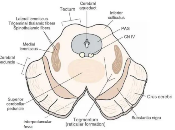
PDis a progressive, neurodegenerative disease that affects the nerve cells of thepars compacta portion of the substantia nigra (SN) situated in the mesencephalon (Figure 2.6). The SNis divided into two anatomical areas that present distinct functions -Substantia

2 . 2 . PA R K I N S O N ´ S D I S E A S E

Nigra pars compacta (SNc)andSubstantia Nigra pars reticulata. However, only theSNcis directly associated with PD[10]. TheSNc neurons produce neurotransmitters - dopamine – which are responsible for controlling motor functions. The dopamine is then released by the SNc to the striatum - brain structure that has control over the motor information exchange between the spinal cord and the brain [11]. Another important characteristic of PD is the degeneration of the locus coeruleus (LC), located in the tegmentum of the upper pons. Such results in a reduction of the neurotransmitter norepinephrine on the frontal cortex, hypothalamus and other brain structures [12].

Figure 2.6: Midbrain section of the mesencephalon illustrating relevant structures for this work, such as the substantia nigra, the interpeduncular fossa and the decussation of superior cerebellar peduncle. Adapted from [13]

C H A P T E R 2 . T H E O R E T I C A L P R I N C I P L E S A N D S TAT E O F T H E A RT

Figure 2.7: Brain anatomy. Brain structures associated with PD: Striatum, Substantia Nigra, Thalamus, Subthalamic Nucleus and Globus Pallidus. Adapted from [11]

The Unified Parkinson’s Disease Rating Scale (UPDRS) is the most accurate and

commonly used rating tool to assess severity and status of PD [17]. The Movement Disorder Society developed this scale, incorporating four main components; Part I evaluates “nonmotor experiences of daily living”; Part II evaluates “motor experiences of daily living”;

Part III registers “motor examination” and Part IV concerns “motor complications.” For each component, there are several questions that are classified using a scale ranging from 0 (normal) to 4 (severe).

PD is an incurable neurodegenerative disease that has few treatments for the attenua-tion of symptoms and trying to slow its progression. The most used anti-Parkinson drug is L-dopa, also known as levodopa, which is a natural dopamine precursor [18]. When PD

treatment using medication is no longer effective in the reduction of motor complications, recurring to surgery with Deep Brain Stimulation (DBS) is a common procedure.

2.2.2 Neuromelanin

Many studies have revealed that theSNcis constituted by neurons with high concentrations of neuromelanin [19]. This concentration linearly increases with age [20], however inPD

patients there is a decrease of NMwhich is believed to be connected with the dopamine loss (Figure 2.8).

Neuromelanin is a dark insoluble pigment found highly concentrated on dopaminergic neurons of theSNc, confined in cytoplasmic organelles. Additionally,NMhas high affinity for metals, particularly iron, and it has been demonstrated that the main neurons who store iron also contain neuromelanin [20]. A few studies have demonstrated that the iron concentration is increased inPD patients [22], possibly as a response to the dysfunctional nigral neurons and consequent iron release. Nevertheless, this topic remains controversial,

2 . 3 . D E E P B R A I N S T I M U L AT I O N

Figure 2.8: Midbrain sections showing the neuronal loss in a PD brain (left) and a healthy subject brain (right). The neuronal loss in the SN of the PD brain can be seen due to the neuromelanin’s properties. Adapted from [21]

since other published studies did not find significant differences in iron concentration between PD and controls [23].

Due to its composition,NMseems to have two very distinct roles: protective and toxic. It has a protective function because of its antioxidant properties that defend the cells from redox active metals. However, when the neuromelanin-containing neurons die,NM

is released to the surroundings where, due to its insolubility, it stays and can potentially release metals and toxic compounds that may damage other tissues and worsen PD[20].

2.3

Deep Brain Stimulation

2.3.1 Introduction to the technique

DBS is a commonly used treatment for patients with PD [24,25]. This technique delivers electrical stimulation to deep brain target structures, such as the STN, via electrodes and an Implantable Pulse Generator (IPG) implanted into a subcutaneous pouch in the subclavicular area (Figure 2.9).

It is believed thatDBSstimulates axons of the STN, triggering a sequence of events that leads to a dopamine release of the SNneurons. WhenSTNstimulation occurs, either excitatory glutamatergic inputs are sent directly to the SNdopamine cells or excitatory cholinergic/glutamatergic inputs are sent indirectly through thePedunculopontine

Tegmen-tal Nucleus (PPT) to theSN [27] (Figure 2.10). With this, there is an enhancement of

dopamine release from the SNneurons to the striatum, motor control is slowly regained and thus an improve inPDsymptoms can be achieved [27].

A series of studies have been developed with the aim of exploringDBS effects onPD

patients [24, 25], mostly inspired in investigating the safety of these patients with DBS

systems implanted.

C H A P T E R 2 . T H E O R E T I C A L P R I N C I P L E S A N D S TAT E O F T H E A RT

Figure 2.9: Medtronic Deep Brain Stimulation System components. Adapted from [26].

Figure 2.10: Illustration of the STN electrical stimulation showing the effects on PPT and SN, which lead to dopamine release on the striatum. Adapted from [27].

Generator (IPG) and extension cables that connect these components. Each electrode

has four metal contacts with neural tissue. When voltage is induced, either through a single contact and the IPG- monopolar stimulation - or between two contiguous contacts - bipolar stimulation -, current is produced and flows to the target tissues [28].

2.3.2 Safety Concerns

The main safety concern withDBSsystems inMRIis the sudden increase of temperature on the electrode contacts. This temperature rise results from the effect of the RF pulses applied during the acquisition of theMRIon the DBSsystem, also known as the antenna effect [29]. The antenna effect suggests that the extended cables used inDBSact as antenna wires, which are sensitive to the electric component, as opposed to the magnetic component of the RF radiation used in MRI. When the electromagnetic waves reach the antenna, they have associated electric charges and consequently currents. When resonance occurs, these currents flow to the tip of the antenna, where the electric energy stays concentrated,

2 . 3 . D E E P B R A I N S T I M U L AT I O N

Figure 2.11: The Medtronic 3389 DBS electrodes for bilateral stimulation. Each electrode has four metal contacts spaced between each other. Contacts 0 and 8 are the deepest. The arrows represent the extension cables that connect the electrodes to the IPG. Adapted from [28].

resulting in a localized increase of temperature [30].

Two case studies reportedMRImaging-related accidents in patients with DBS systems implanted [31, 32]. Thus, establishing the safety of performing MRI in patients with subthalamic deep brain stimulators became a priority. Nowadays, safety considerations have to be taken into account when performing MRI scans in patients with neurostimulation systems, namely the impossibility of using 3T MRI systems on these cases [33]. The strong magnetic field characteristic of 3T machines implies an increase of the RF pulses frequency and consequently induces more easily a temperature rise on the tissues, which was demonstrated to be harmful [30]. An evaluation of safety using 1.5T MRIwas performed and it was proved that the temperature increase can be controled at said field strength [34]. Since then, numerous 1.5TMRIsequences have been tested confirming that it is safe to obtain these images on patients with implanted neurostimulators [35], as long as a few additional restrictions are obliged.

The most important considerations, in addition to the usage of a 1.5T MRI scan, are: to turn off the DBS stimulation while performing the scan and when defining the parameters for theMRIsequence, theSpecific Absorption Rate (SAR)presents a threshold imperative to respect [33]. These limits are described in Table 2.1. The SAR measures the rate at which energy is absorbed by the body. The purpose of this metric is to indirectly evaluate the temperature increase on body tissue, caused by the RFenergy deposition [35]. SARis proportional to the power of 2 of the resonance frequency, as shown in equation 2.5 [36]:

SAR_∝B2

0∗(f lip angle)2∗(RF duty cycle)∗(patient size) (2.5)

C H A P T E R 2 . T H E O R E T I C A L P R I N C I P L E S A N D S TAT E O F T H E A RT

The SAR estimate is, however, dependent on the patient’s size and mass and it varies according to the model used by each MRI manufacturer [38]. Therefore, the B1+RM S

parameter was recently presented as a more accurate measure of potential implant heating in MRI scanners [39] (Table 2.1). B1+RM S is the time-averaged RFmagnetic field

compo-nent responsible for the creation of anMRimage. B1is the magnetic field generated with

the application of RF pulses, which presents rotating components, the positive one being responsible for the protons flip that generates the MR images. B1+RM S is thus a measure

of the magnitude of the positive rotating component of theB1magnetic field necessary to

create an MRI in 10 seconds [38].

SAR (W/Kg)

B1+RM S (µT)

Whole body Head

3T ≤2 ≤3.2 ≤2.8

1.5T with DBS system ≤0.1 ≤0.1 ≤2

Table 2.1: SAR andB1+RM S maximum values that ensure safe examinations - at 3T and

at 1.5T with implanted DBS systems.

2.4

NM-MRI sequence

In 2006, Sasaki et al [40] developed the first MRIsequence capable of identifyingin vivo

neuromelanin-containing structures, namely SN andlocus coeruleus, from the surrounding brain. The proposed NM-MRIsequence was a T1-weightedFSE applied at 3T.

The images corresponding to this sequence revealed band-like high signal areas in the posteromedial portion of the cerebral peduncle visualized at the level of the midbrain (Figure 2.12b) [40]. This finding agrees well with the presence of NM in the SN, in in vivo slices (Figure 2.12a), suggesting that the NM-containing SNneurons are related to the high-signal intensity. This relation was later confirmed by another study, which noted a clear correlation between the signal intensity and the density of the NM containing neurons, for different parts of theSN[41]. Furthermore, the signal intensity inPDpatients was revealed to be reduced in comparison with healthy subjects, in agreement with the progressive loss of SN neurons that occurs on PDpatients.

A possible explanation for the obtained contrast is that NM’s paramagnetic properties facilitate its orientation with the direction of the external magnetic field, resulting in an acceleration of the T1 relaxation and thus explaining the high signal intensity of the NM

[40]. Additionally, it was suggested that the high iron concentration in the SN may have contributed to theT1-shortening effects [40]. Although a posterior study found no apparent

influence of iron deposition on the signal intensity of the SN [41], the influence of iron in

MRI is still not completely understood [43].

Another essential requirement for the correct identification of the SN signal is the choosing of the slice orientation. The sections must be set it the oblique axial plane, oriented perpendicular to the fourth ventricle floor, starting from the inferior border of

2 . 4 . N M - M R I S E Q U E N C E

Figure 2.12: Neuromelanin-sensitive and conventional magnetic resonance images of the

substantia nigra. Axial sections at the level of the midbrain; macroscopic specimen (a) and MR images obtained at 3T with NM-MRI (b), T1-WI (c), T2-WI (d) and PDn-WI (e). The arrows on (a,b) indicate the SNc. On (d) the large arrow points to the SN and the small arrow to peduncular fibers. The arrowheads on (e) point to the SN. Adapted from [42].

the pons to the posterior commissure region [43] (Figure 2.13). The slice orientation in NM-MRI is particularly important due to the small number of slices, three at best, in which the SN is visible. Additionally, in NM-MRI sequences the slice thickness is usually larger than the resolution, which can cause partial volume effects and hence potentially hinder the SN detection. For these reasons, slight alterations in the slice angulation could alter significantly the delineation of the SN in the MR images, emphasizing the importance of choosing a correct slice orientation.

Figure 2.13: Correct slice orientation of a neuromelanin-sensitiveMRIsequence. Adapted from [43].

ConventionalT1-weightedSE sequences have failed to capture NM-generated signals

(Figure 2.12c). Also, on T2-WI, the SN region shows low signal intensity and contrast

C H A P T E R 2 . T H E O R E T I C A L P R I N C I P L E S A N D S TAT E O F T H E A RT

pars reticularis (Figure2.12e) [44].

Meanwhile the majority of studies have been applyingT1-weightedFSEsequences at

3T (Table2.2) with good spatial resolution [45]. TheSNRat 3T is twice as higher than at 1.5T and at 3T the relaxation timeT1of the brain tissue is higher. This implies a signal

suppression of the surrounding brain tissue caused by the longerT1[46] and, consequently,

an enhancement of the neuromelanin-contrast [40]. Additionally,FSEsequences are associ-ated with increased incidental Magnetization Transfer (MT)effects [47]. All these factors contribute to the successful visualization of NM-containing tissues but the key factor is believed to be the MTeffects that result from the multiple applications of RFpulses.

MT is a process where spins transfer energy (magnetization) from bound protons to free protons. Usually the MR signal reflects only the magnetization associated to free protons due to their long T1 and T2 values. The bound protons, which have very short T2 values, reach magnetization saturation very quickly. In the case of FSE sequences, the application of multiple 180º pulses facilitates the magnetization saturation of the bound protons leadind to a magnetization transfer to the free protons. With this, a reduction in the MR signal associated to the bound protons occurs, resulting in an enhanced contrast [48].

Recently, a 3D Gradient Echo sequence with an additionalMTpre-pulse was proposed for visualizing NMat 1.5T [49] but no subsequent studies have been reported at this field strength. This sequence revealed to have the needed resolution for enabling the observation of SNand locus coeruleus. The acquisition parameters of the referred sequence, as well as of previously mentioned related NM-MRI sequences are presented in Table 2.2for a more easy comparison.

With theGEsequence, the determinant factor for a good achievement ofNMcontrast was the application of aSlice Selective Off Resonance Sinc (SORS)pulse with Saturation

Transfer Contrast (STC), which generates MT contrast. When the surrounding brain

tissue signal is suppressed by the STC, the contrast between this tissue and the NM is enhanced, also due to the T1 reduction caused by theNMand confirming the theory that

MT effects are reduced in tissues that contain paramagnetic substances [50]. This study demonstrated that it is possible to visualize NMcontrast at 1.5T due to the applied MT pulse. Another study [51] corroborated this theory and showed thatGE sequences with

MT preparation pulses are able to produce better contrast than FSE sequences, which rely solely on incidental MT effects [52]. Such is consistent with the observation that most NM-MRI contrast is derived from MT effects. In [53], a NM-MRI protocol with a single slice of the SN was tested and it was not possible to distinguish the SN from the surrounding brain tissues, thus corroborating the importance of MT effects in NM-MRI.

2

.4

.

N

M

-M

R

I

S

E

Q

U

E

N

MRI sequence

MRI protocol

TR TE

Turbo factor FA FOV Pixel size Matrix Slice thickness Acquisition time

(ms) (ms) (º) (mm2_{) (mm) (mm) (min:sec)}

2D

Sasaki - 3T T1W FSE 600 14 2 90 220×220 0.31×0.36 512×320* 2.5 12

Schwarz - 3T T1W FSE 688 9 2 90 - 0.47_×0.47 - 2.5 12

Chen - 3T T1W FSE 600 12 2 90 162×200 0.39×0.39 416×512 3 12:34

Chen - 3T GE 260 2.68 - 40 162×200 0.39×0.39 416×512 3 12:39

3D Ogisu - 3T T1W FSE 13 2.2 59 20 220×220 0.69×0.93 320×236 1 6:55

Nakane - 1.5T GE 40 6.8 - 20 200×200 0.62×0.62 320×320 2 8:20

Table 2.2: MRI protocols of several neuromelanin-sensitive MRI sequences. Sasaki et al [40] developed the first NM-MRI using a 3T scanner. Similar sequences have since been developed using 3T MRI systems; Schwarz et al [54] tested a T1-weighted FSE similar to Sasaki’s with an inversion recovery pulse; Ogisu et al [55] developed a 3D sequence with a MT pulse. Chen et al [51] compared a T1W FSE sequence similar to the previously described by Sasaki with a GE sequence with an additional MT pulse. Nakane et al [49] developed the first NM-MRI sequence at 1.5T using a 3D GE sequence with a MT pulse. *In this case, the acquisition matrix is presented, whilst the pixel size was calculated with the reconstructed matrix.

C H A P T E R 2 . T H E O R E T I C A L P R I N C I P L E S A N D S TAT E O F T H E A RT

2.5

Statistical Tests

2.5.1 Non-parametric Tests

When performing statistical tests, two contradictory hypotheses are stipulated. These statistical hypotheses are conjectures about the distribution of one or more random vari-ables. The first hypothesis, designated as null hypothesis (H0), assumes that there is no

difference between the parameters. The second hypothesis or alternative hypothesis is denoted as H1 and represents the opposite of H0 [56].

The goal of a statistical test of an hypothesis is not to determine whether the statement is true or not, but to determine if it is consistent with the observed sample. As so, the null hypothesis should only be rejected when the observed data has a very low probability of being true. By defining ap-value lower than 0.05 as significant, if the obtained result is indeed significant (p < 0.05) the null hypothesis is rejected. Otherwise, if (p ≥0.05),H0

is supported [56].

There are two main statistical tests: parametric and non-parametric tests. Non-parametric tests are applied when no assumptions that the data is influenced from a given probability distribution are made, as opposed to parametric tests. Non-parametric tests are usually used in cases with small samples (n < 30), also these are more accurate than parametric tests when the normality of the data cannot be assumed [57].

For these reasons, in the present study, the following non-parametric methods were applied: Friedman test and Wilcoxon signed rank test.

The Friedman test is used to test for differences between three or more related groups, where the hypotheses to be tested are [58]:

• H0: All groups came from the same population or from populations with the same

distribution;

• H1: Not all groups have the same distribution.

The Wilcoxon signed rank test is used to compare paired samples. The samples must be dependent within the par (paired samples) and independent between pairs [59]. The tested hypotheses of the Wilcoxon test are:

• H0: The median difference between paired samples is zero;

• H1: The true location shift is not equal to zero.

2.5.2 Intraclass Correlation Coefficient

For any measurement procedure to be used in clinic practice, reliability of the method has to be established. The chosen method for analyzing test-retest reliability of the semi-automatic algorithm is the Intraclass Correlation Coefficient (ICC). This is the only

2 . 5 . S TAT I S T I C A L T E S T S

measure of reliability that measures both correlation and agreement between measurements [60].

The ICC can assume different forms according with the type of study that is being performed. Its values always range from 0 to 1, with values closer to 1 representing stronger reliability. As in the present study test-retest reliability is being assessed, ICCestimates and their 95% confidence intervals were calculated based on a single measurement, absolute agreement, 2-way mixed-effects model, as defined by McGraw and Wong [61].

2.5.3 Bland-Altman Method

In this study, the agreement between two methods of measurement - SN areas taken with the 1.5T sequence and with the 3T sequence - had to be assessed. To do so, the graphic statistical procedure proposed in 1983 by Altman and Bland [62] was performed. This method evaluates the agreement between two quantitative measurements by calculating the mean difference and limits of agreement of the said measurements.

The resulting graphic is a scatter plot XY, considering that the obtained measurements from the two different methods are represented by the variables A and B, in which the Y axis represents the difference between the paired measurements and the X axis the average of those measures (Figure 2.14). The Bland-Altman plot has a confidence interval of 95 %, meaning that 95 % of the data should lie within±1.96SD(standard deviation) of the mean difference. The bias is represented by the gap between the mean difference of two measurements and the X axis, which corresponds to zero differences [63].

Figure 2.14: Example of a Bland-Altman plot of differences between method A and BVs.

C H A P T E R 2 . T H E O R E T I C A L P R I N C I P L E S A N D S TAT E O F T H E A RT

While other agreement analyses, such as the ICC, have defined criteria to evaluate the level of agreement between measurements, the Bland-Altman method only provides the intervals of agreement and it us up to the user to interpret whether those limits are acceptable or not.

C

h

a

p

t

e

r

3

Va l i d a t i o n o f a 1 . 5 T N M - M R I s e q u e n c e

Neuromelanin-sensitive MRI is a promising technique to allow the visalizationin vivoof the pathological changes inNM-containing structures that occur in degenerative disorders and has recently also been applied to psychiatric disorders [42]. The majority of studies have applied NM-MRI at 3T due to its improved resolution and SNR. However, availability and safety reasons due to patients with implantable devices such as neurostimulators, cardiac pacemakers and cardioverter-defibrillators may prevent imaging at this field strength [64,

65]. This chapter describes the development of a 1.5T NM-MRI sequence through adapta-tion of the commonly used 3T NM-MRI sequence in clinic practice. These two sequences were compared using a semi-automatic segmentation algorithm applied to the SN, aiming to establish the feasibility of the developed 1.5T sequence. Additionally, differences in the contrast ratio of the tested sequences were assessed.

3.1

Materials and Methods

3.1.1 Sample Description

Twelve individuals (4 males and 8 females), with ages ranging from 38 to 85 years (mean age: 62.5_±13.1 years) were included in the present study. From this pool, seven subjects were diagnosed with PD by a movement disorders specialist according to the PD UK Brain Bank criteria [66]. The remaining five subjects had still an undetermined diagnosis but presented movement-related disorders. Patients were recruited from the Movement Disorders Unit of Hospital of Santa Maria-Lisbon.

C H A P T E R 3 . VA L I DAT I O N O F A 1 . 5 T N M - M R I S E Q U E N C E

3.1.2 Imaging Protocol

To develop a 1.5TNM-MRIapplicable in clinic practice and with an adequate reproducibil-ity and image contrast, the 3T T1-weighted FSE sequence currently used at Hospital of

Santa Maria-Lisbon was the starting point from which the 1.5T sequence was adapted from. The necessary changes are discussed next in subsection 3.1.2.1.

The 3T sequence had the following acquisition parameters: repetition time/echo time of 606/10ms; turbo factor of 3; FOVof 220×190 mm2_{; matrix size of 548×474 (pixel size}

of 0.40×0.40 mm2_{); slice thickness of 2.5mm with no gap; four averages;Parallel Imaging}

(PI) with reduction factor of 1.5 and an acquisition time of 8:35 min.

The acquisition parameters of the 1.5T sequence were: TR/TE of 600/10ms; turbo factor of 3; FOV of 220×180mm2_{; matrix size of 440×361 (pixel size of 0.50×0.50 mm}2_);

slice thickness of 2.5mm with no gap; four averages; no PIacceleration, and an acquisition time of 9:45 min.

Both systems usedT1–weighted FSEsequences and all images were acquired with an

8-channel SENSE head coil. All data were acquired with a 3T MRI (Achieva 3.0, Philips Medical Systems, Best, Netherlands) and a 1.5T MRIsystems (Intera 1.5, Philips Medical Systems, Best, Netherlands). Each subject underwent a single scan in each MRI system with both acquisitions being performed on the same day, by a random order according to the availability.

In both cases, the sections were carefully set in the oblique axial plane perpendicular to the floor of the fourth ventricle, starting from the posterior commissure to the inferior border of the pons.

3.1.2.1 Analysis of the acquisition parameters

The changes applied to the original sequence were made with the purpose of ensuring sufficient resolution on the 1.5T sequence to enable the visualization of the SN. Adding to this, an effort to change as few parameters as possible was made so that at the time of the analysis, variability sources will have been reduced.

In order to compensate the reduced SNR typical of 1.5T images, the size of the ac-quisition matrix was reduced, leading to a slightly coarser pixel size (0.5x0.5 mm2_{) and}

consequently a smaller spatial resolution was obtained. The FOV was slightly decreased, although it was not significant so that it would change spatial resolution. These slight changes in the FOV values are very common in the clinic considering that this parameter has to be adjusted according to the head size of each individual patient.

Despite the potential change on T1 contrast due to the alteration of field strengths, TR and TE were kept along the same values, as we expected the intrinsic MT effects to be dominant. The time of repetition was slightly reduced. Nevertheless, this reduction did not have much of an impact on the acquisition time due to the deactivation ofSENSitivity

Encoding (SENSE).

3 . 1 . M AT E R I A L S A N D M E T H O D S

SENSE is a parallel imaging technique that enables the reduction of the number of phase encoding steps and reconstructs the missing data taking into account the coil sensitivity variation between channels [67], thus enabling a shorter acquisition scan (8:35 min). However, the reduced image information necessary to obtain a shorter scan time results in a diminished SNR related to the reduction factor:

SN RP I=

SN R √

R (3.1)

, where R represents the reduction factor by which the number of k-space samples is reduced. Therefore, considering that 1.5T sequences predictably present a worse SNR when compared to 3T sequences, parallel imaging was not applied to the developed 1.5T sequence and its acquisition time increased (9:45).

3.1.3 Imaging Analysis

Image processing was performed using the OsiriX program (Version Lite) [68]. This program combines visualization features of medical images with various processing tools and is more easily applicable in clinic practice than similar implemented processing in Matlab.

To assess if the developed 1.5T NM-sequence is effective and comparable to the al-ready existing 3T NM-sensitive MRI sequence, as well as able to detect changes in the neuromelanin-containing structures, it is essential to define a method that allows quanti-tative measurement of the SN.

There have been several reports [51,55,69] ofSNquantification with different segmen-tation methods. Most of these studies used two-dimensional (2D) sequences. However, there were divergences regarding the type of SNmeasurements – area [54,69] or volume [51,70]. Since 2D segmentation of a single slice is simpler and faster and therefore more easily included in clinic practice, the SNquantification in this study was made through measurements of the SN area from a single slice. Additionally, the thick slices used in the study (2.5mm) that are necessary to ensure sufficient SNR, can lead to partial volume effects thus originating subjective SN volume measurements.

Once the type of SN measurement is defined, there are two possible segmentation methods – manual or automated. In the present study, a semi-automated segmentation method optimized in a previous Master Thesis [71] was applied. Furthermore, in order to evaluate the repeatability and feasibility of the algorithm, manual segmentation of the SN

was used as gold standard. All the segmentation process is described next in subsection

3.1.3.1.

3.1.3.1 Segmentation method

C H A P T E R 3 . VA L I DAT I O N O F A 1 . 5 T N M - M R I S E Q U E N C E

there were doubts in slice selection owing to the fact that the NM-SN area was visible on more than three slices. For these two subjects only, slices that were visually similar at 1.5T and 3T were chosen.

a Lower midbrain b Center midbrain c Upper midbrain

Figure 3.1: Axial sections at different levels of the midbrain showing thesubstantia nigra as a hyper intense signal area. The middle slice (b) was the one chosen for SN measurements.

In order to compensate for the reduced SNR present in NM-MRI that can have an effect on segmentation, aGuassian blur filter, which is incorporated in the OsiriX features, was applied to the selected slice (Figure3.2b).

a Original image b Filtered image

Figure 3.2: Selected axial middle slice for SN measurements before (a) and after (b) the application of the Gaussian blur filter, showing a clear blur effect of the applied filter.

The Guassian blur filter uses a Gaussian function to calculate the kernel (Figure 3.3) that will be applied to each image pixel. During the image convolution, the pixel that is being analyzed is given the highest weight – corresponding to the center pixel of the mask, whilst the neighboring pixels which are covered by the mask, are given increasingly lower weights as the distance between them and the main pixel increases. This filter is commonly used in image pre-processing because it reduces the noise in the image, thus facilitating the segmentation that follows. Additionally, compared to the other filter types already implemented within Osirix, the Gaussian blur filter was demonstrated in [71] to have the best performance in the SNsegmentation. The used filter has a kernel dimension

3 . 1 . M AT E R I A L S A N D M E T H O D S

of 5×5 pixels and a Full Width at Half Maximum (FWHM)of 2 pixels.

Figure 3.3: Representation of the colored image corresponding to the 5x5 Gaussian blur kernel. The color-bar on the right shows how the data values correspond to the image, with the highest weight being given to the center pixel.

With the selected filtered image displayed, there are some adjustments that need to be done before the application of the segmentation algorithm. The OsiriX software enables to modify the displayed contrast, thereby facilitating the user in visualizing the SN area, as well as zooming in and rotating the image - all helpful tools for the correct identification of the substantia nigra.

The OsiriX 2D semi-automatic segmentation tool has three available algorithms: Thresh-old,Neighborhood and Confidence. This last algorithm was chosen as it was shown in [71] to be the most practical and efficient method for segmentation of the NM-corresponding area. The Confidence algorithm requires the definition of three parameters, which define the inclusion criteria: multiplier, number of iterations and initial radius, whose correspond-ing values for the correct identification of the SN were, as defined in [71] - 2,2 and 1, respectively (Figure 3.4).

The Confidence algorithm is based on a commonly used segmentation technique –

Region growing. This technique enables growth of regions that were previously marked withseed regions. That is, starting with the initial selected set of pixels, the neighboring pixels are posteriorly evaluated based on the inclusion criteria to decide whether they should be included in the segmented region or not.

Owing to the fact that the algorithm is based on Region growing, the relevance of developing sequences that successfully depict the neuromelanin-containing structures and optimizing image contrast is particularly relevant. A possible source of concern is the placing of the seed region, which influences the identification of the Region-of-Interest

(ROI). Thus, to minimize the seed placing error and consequent variability of the ROI, a

C H A P T E R 3 . VA L I DAT I O N O F A 1 . 5 T N M - M R I S E Q U E N C E

Figure 3.4: OsiriX segmentation tool interface that enables the definition of the segmenta-tion algorithm and respective parameters. In this study, the chosen segmentasegmenta-tion algorithm was Confidence and its parameters were 2 Multiplier, 2 Number of Iterations and 1 -Initial Radius.

After the application of the semi-automatic algorithm, it was common for the segmented

SNregions to present gaps (Figure3.5b). Yet, anatomic examinations have shown that the

SNis a structure which does not present gaps. For this reason, a last filter -Brush closing -was applied and with this, the gaps that were not being accounted for the area calculation became filled (Figure3.5c). Finally, with the semi-automaticSNregion correctly delineated, the corresponding ROIwas saved as well as some of its characteristics, such as area and mean signal intensity, which are available in the OsiriX software.

SN segmentation using the semi-automatic tool explained above was performed three times for each side of the brain in order to assess test-retest reliability. The three repeated measures of theSN ROIs were performed on different days to avoid biasing.

The left and right ROIs of each image were considered independent regions, as it is common in PDfor one side to present a more accentuated loss of dopaminergic neurons of the SN, making a total of 24 SNregions to be studied. For each SN region, manual segmentation was also performed on a different day. TheSN manual contours were made resorting to an OsiriX tool that enables the user to freely draw over the image, in order to obtain the sought segmented region, and adjust the said region if needed (Figure 3.6). The manual ROIs were all validated by a certified neuroradiologist (Dr. Sofia Reimão) and saved to be used as gold standard.

3 . 1 . M AT E R I A L S A N D M E T H O D S

a Pre-segmentation bConfidencealgorithm

c AfterBrush closing

Figure 3.5: SN semi-automatic segmentation process. First a line is drawn crossing the interpeduncular fossa (a). Then, a pixel along the line is chosen and the Confidence

algorithm generates the region-of-interest accordingly (b). At last, the Brush closing filter is applied to ensure that the selected SN area is completely filled (c).

a Manual segmentation b Semi-automated segmentation

C H A P T E R 3 . VA L I DAT I O N O F A 1 . 5 T N M - M R I S E Q U E N C E

3.1.3.2 Similarity Analysis

The analysis of the SN areas is very effective to evaluate quantitative differences in the dimensions of the ROIs, thus enabling the assessment of neuropathological changes. Never-theless, there is no information regarding spatial distribution of the SNsegmented regions. A very common method used in medical images to assess the reproducibility of seg-mented regions is theDice Similarity Coefficient (DSC)calculation [70,72]. This coefficient quantitatively measures the spatial overlap between two segmented regions, complementing the analysis of the comparison between SNregions.

In this study, the overlap between the semi-automaticSN ROIand the reference manual segmentation was determined using the DSC:

DSC= 2 area(SNsa∩SNm)

area(SNsa) +area(SNm)

(3.2)

where area(SNsa) and area(SNm) representSN areas for a semi-automaticROIand

corresponding manually-segmented region, respectively, and ∩ represents the intersection operator. The DSC ranges from 0, where the segmented regions do not intersect at all to 1, which indicates exact overlap.

An application in Matlab (R2016, The Math Works, Natick, MA, USA) was created to estimate the DSC. The developed interface (Appendix A.1) enables the loading and visualization of two DICOM images, the visualization of the two segmented regions overlap with two possibilities – just showing the region that resulted from the overlap (Figure3.7c) or displaying the two initial regions and its overlap in different intensities (Figure 3.7d) -and calculates the DSC. Additionally, the application allows the user to zoom in and out on all images and to save the resulting image.

The two DICOM images that were compared with the Matlab application contained a semi-automatic SN region and the other its corresponding manual segmentation. For the application to work, these images had to be taken from the OsiriX program displaying solely the isolated segmented regions. Considering this, the developed script treats the image as binary and assigns the value 1 (white) to every pixel that does not have intensity 0 (black), displaying the region-of-interest as white and the surroundings as black (Figures

3.7a and3.7b).

3.1.3.3 Image contrast Analysis

FSE NM-MRI sequences rely solely on incidental MT effects to distinguish the NM

-containing structures. Furthermore, image contrast at 1.5T is expected to be diminished when compared to 3T. Considering this, it is imperative to evaluate the obtained NM -related contrast in order to assess the feasibility of the 1.5T FSE sequence that is being tested.

Because SN segmentation is performed after application of the Gaussian blur filter - the first step of the segmentation pipeline – described previously in 3.1.3.1, it would

3 . 1 . M AT E R I A L S A N D M E T H O D S

a Binarized semi-automated region b Binarized manual segmented region

c Binarized overlap region d Two segmented regions and its overlap

Figure 3.7: Segmented regions after binarization (a,b) and two available display options for visualizing the resulting overlap (c,d) - with the Matlab application for DSC calculation.

be interesting to assess Contrast Ratio (CR) differences between field strengths after the filter application. However, knowing that image filtering may potentially affect the contrast, it is also necessary to evaluate the significance of these differences. Thereby,CR

was measured both before and after the filter application, keeping the used ROIs in the exact same positions. Additionally, in order to assess whether differences in CRaffect the segmentation, CR was calculated on the same slices that were used to measure the SN

areas – for both field strengths.

To evaluate the CR, the fraction ISN/IDP was calculated where ISN represents the

mean signal intensity of two 6.0mm2_{squareROIs (one for each side of the brain) located in}

theSN portion matching an imaginary line crossing the interpeduncular fossa. IDP is the