Julião Soares de Souza Lima1, Felipe Pianna Costa2, Alexandre Cândido Xavier1, Rone Batista de Oliveira3, Samuel de Assis Silva4
(Recebido: 23 de setembro de 2013; aceito: 2 de dezembro de 2013)
ABSTRACT: GIS techniques have been used in many agricultural crops to study and assess the causes of spatial and temporal variability in production. The spatial and temporal variability of the canephora (conilon) coffee productivity was analyzed in the present work in three consecutive agricultural years (harvests) using geoprocessing techniques. A sampling grid with 109 georeferenced points was built with five plants per point. Significant differences in productivity were observed, with the lowest productivity recorded for the harvest 3 in 93.5% of the area. The productivity index (YI) varied from -18.0% in harvest 2 to harvest 1 and from -57.0% in harvest 2 to harvest 3, showing increasing decrease between different harvests.
Index terms: Geostatistics, soil management, semivariograms.
VARIABILIDADE ESPACIAL E TEMPORAL DA PRODUTIVIDADE DO CAFEEIRO CANEPHORA
RESUMO: Em várias culturas, tem-se utilizado técnicas de geoprocessamento com intuito de estudar e interpretar as causas da variabilidade espacial e temporal da sua produção. Este trabalho foi desenvolvido objetivando-se analisar a variabilidade espacial e temporal da produtividade do cafeeiro canephora (conilon) em três safras consecutivas, utilizando técnicas de geoprocessamento. Uma malha amostral foi construída com 109 pontos georreferenciados, considerando cinco plantas por ponto. As produtividades apresentaram diferenças significativas, com menor produtividade na safra 3, em 93,5% da área. O índice de produtividade (IP) ficou da safra 2 para a 1 em -18,0% e da safra 3 para a 2 em -57,0%, mostrando redução crescente entre as diferentes safras.
Termos para indexação: Geoestatística, manejo do solo, semivariograma. 1 INTRODUCTION
Predicting and mapping the spatial and temporal variability of the productivity areas allows crop producers to improve their planning of agricultural activities.
The analysis of spatial and temporal variability of the productivity has brought about the precision agriculture aiming at optimizing lime and fertilizer application, identifying regions with different productivity and minimizing costs and environmental impacts. According to Milani et al. (2006) Precision Agriculture is a crop management strategy that assess management zones considering their different productivity potential.
For some time now, the productivity determination in mechanized harvesting of various crops has been successfully accomplished. Productivity monitoring is associated with GPS’s
1Universidade Federal do Espírito Santo/UFES - Departamento de Engenharia Rural – DER/CCA - Cx. P. 16 - 29500-000 Alegre - ES - [email protected]
2Universidade Federal do Espírito Santo/UFES - Pós-graduação em Produção Vegetal - Cx P. 16- 29500-000 - Alegre - ES [email protected]
3Universidade Estadual Norte do Paraná/UENP - Cx. P. 261 - 37.200-000 – Bandeirantes - PR [email protected] 4Universidade Estadual de Santa Cruz/UESC - Departamento de Ciências Agrárias e Ambientais - 45662-900 - Ilhéus -BA [email protected]
coupled to the harvesting equipment, originating real time productivity maps of the considered area. However, the use of this technology is limited in some crops such as coffee, grown in large areas in mountainous regions. Molin (2002) used productivity maps to define management units with satisfactory results.
According to Miranda et al. (2005) the existing variability in a specific area can influence production factors related to nutrient availability, for example. If spatial variability is observed for these factors and for crop productivity, the localization of high and low productive potential sites might bring benefits when localized management strategies are used. Ferraz et al. (2012) assessed and found spatial variability in the productivity of the arabica coffee and in soil chemical properties. These results suggested the need of productivity maps for a satisfactory management of precise management practices.
The following theoretical models were tested in the spatial analysis: spherical, exponential and Gaussian for the definition of the following parameters: nugget effect (C0) that represents the discontinuity of the semivariogram at distances larger than the smallest distance among; sill (C0+C), representing the value at which data variance is stabilized, therefore, the sum of: nugget effect (C0) + contribution (C); and range (a) of spatial dependence, corresponding to the spatial lag in which the samples are independent (VIEIRA et al., 2009).
The degree of spatial dependence (DSD) was calculated by the ratio [C0/(C+C0)] × 100, according to Cambardella et al. (1994). The values of DSD up to 25%, between 25% and 75% and above 75% represent strong, moderate and weak spatial dependence, respectively.
The highest determination coefficient of the semivariograms (R2) and the lowest sum of squared residuals (SSR) were used as criteria for the choice of the theoretical model. As a definitive criterion, however, we chose the model with the highest and most significant correlation coefficient among the observed and estimated values for cross-validation (LIMA et al., 2008; LIMA; OLIVEIRA; SILVA, 2012).
Following the confirmation of productivity spatial dependence in the different harvests, the ordinary kriging interpolation technique was used to estimate values at unrecorded locations. According to Grego and Vieira (2005) the kringing technique produces estimates of values without bias and with minimum deviations in relation to the known values.
The quantitative diagnosis of productivity in the area was performed using geoprocessing resources (GIS), which allowed the determination of the degree and extent of the alterations occurred in the different harvests.
From the maps of productivity spatial distribution in each evaluated year, we generated loss and/or gain maps (MPG) or productivity levels (Nprod) between the harvests (equation 02), indicating regions with different productivity.
where MPG is the loss and/or gain in productivity; Mp(n) is the map of the spatial productivity distribution in harvest n, and Mp(n-1) The application of methodologies to define
productivity-based management zones has been subject of various studies for different cultures, considering their spatial and temporal variability. The aim of this study was to analysis the spatial and temporal variability of the canephora (conilon) coffee productivity in three consecutive agricultural years (harvests) using geoprocessing techniques.
2 MATERIAL AND METHODS
The experiment was carried out at in the municipality Cachoeiro de Itapemirim-ES in an experimental area cultivated with the conilon species (Coffea canephora Pierre ex Froehner) of the cultivar Robusta Tropical. The coffee plants were spaced 2,9 x0, 90 m in an area with altitude ranging from 100 to 150 m, in the following coordinates: 20 ° 45 ‘17” South latitude and 41 ° 17’8, 86” West longitude of Greenwich.
An irregular grid was delineated in the central area of the crop, with 109 georeferencing sampling points and approximately 10 m spacing along the coffee plant line. Each sampling point consisted of five coffee plants. The studied harvests were the fifth, sixth and seventh, denominated harvest 1, 2 and 3.
The hand-picked coffee at each sample point was stored and identified in bags and sent to the INCAPER laboratory for oven moisture determination, in order to correct the productivity to the standard moisture of 12%, obtaining dry beans. The productivity of the milled coffee (sc ha-1) in each crop was calculated after processing at each sample point.
Geostatistical analyses were used to produce maps of spatial distribution of productivity in the three harvests and to quantify the spatial dependence degree among the samples. In this analysis we opted for the intrinsic stationarity hypothesis, using a semivariogram, equation 01 (LIMA; SILVA; SILVA, 2013). If no sill is defined in the semivariogram, the trend analysis will be carried out.
( )
( )
∑
( )[
( )
(
)
]
=+
−
=
N h i i ih
x
Z
x
Z
h
N
h
1 22
1
*
γ
Eq 01where: γ*(h) is the estimated semi-variance and N(h) is the number of pairs of measured values Z (xi) and Z (xi + h), separated by a distance vector h.
is the map of the spatial productivity distribution in harvest (n-1).
The productivity index (YI) from one harvest to another was determined using the interval of each class in the loss and/or gain map (MPG) by the area occupied in the map, from algebraic operations. The quantification of the productivity variation between the different harvests using the productivity index (YI) indicates the increase and/or decrease in productivity between harvests (equation 03).
where: YI is the productivity index of the area; ICi is the class interval for productivity in the maps, and Ai is the class area of a given level of productivity.
3 RESULTS AND DISCUSSION
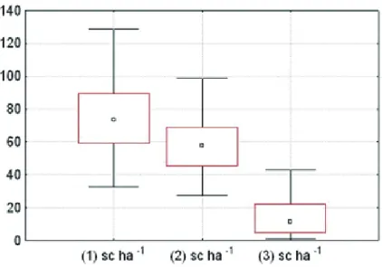
The box plot in Figure 1 shows the central position of the data and the temporal variability of the crop productivity for the milled conilon coffee for the three consecutive years. The position (mean and median) and dispersion (coefficient of variation) measures were 74.8; 73.4; 28.6 to (1), 58.5, 57.3, 28.4 to (2) and 14.4, 11.4, 80.7 to (3) to three consecutive years.
High variability was found for the productivitys of the green coffee (sc ha -1) between the three harvests, with values ranging from 32 to 128 sc ha-1, 27 to 98 sc ha-1 and 1 to 48 sc ha-1 for the first, second and third harvest, respectively.
The productivitys of all harvests presented approximate measures of central tendency (mean and median), positively or right skewed, with a tendency of data concentration skewed to the right, with mean values greater than the median. Productivitys in the different harvests had normal data distribution according to the Kolmogorov-Smirnov (KS) test at (p <0.05).
Based on the results of the Student’s t test (p <0.05), it was found that the productivity was significantly different between harvests. This may have been the result of several factors that played individual or joint roles in reducing the productivity between the harvests, such as climatic conditions,
soil fertility, relief, and cultural practices, but is not evaluated in this study. Barbosa et al. (2006) discussed that the lack of lime application or its insufficient dosage contributes to low productivity values, as was observed in harvest 3. However, little work has comparatively been conducted in line with the initial studies of Weill et al. (1999) on the causal relationships between soil and coffee cultivation in the context of spatial variability.
The analysis of the coefficient of variation (CV) proposed by Gomes (1987) showed that the first two harvests had average variation (10% ≤ CV ≤ 30%) and the third harvest had high variation (CV> 30%). Values of CV with average variation was reported by Silva, Lima and Alves (2010) for conilon and with high variation by Silva et al. (2007) and Silva, Teodoro and Melo (2008) in studies with Arabic coffee productivity.
The theoretical semivariograms for harvests 1, 2 and 3 were defined in the spatial analysis, scaled by data variance, with fitting of the exponential model to the data. The following parameters were set: C0 (0.40; 0.31; 0.04), C0+C (1.20; 1.02; 0.91), range (a) (131.7 m; 20.7 m; 26.3 m), GDE (29%; 30%; 11%) and R2 (90%; 98%; 97%), respectively. Harvest 3 showed strong spatial dependence (GDE <25%), while the remaining harvests had moderate spatial dependence. Harvest 1 had the highest range, indicating greater spatial continuity with moderate spatial dependence (25% <GDE <75%). According to Silva et al. (2010), with the definition of the semivariogram sill, there is an intrinsically stationary process, since there is no variation tendency for productivity with the directions.
The productivity thematic maps of the three harvests are shown in Figure 2.
The productivity maps show that the first two harvests are identified in the higher productivity zones. Higher productivity was observed in the first and second harvests at the top and bottom of the maps, respectively.
For the third harvest, lower productivity was observed in all the studied area, especially in the central part, when compared with the other harvests. In general, the productivity in this harvest was low in relation to the production potential, as shown in the previous harvests.
The productivity temporal variability does not show the same distribution tendency in the area during the harvests. There was, however, alternating productivity zones throughout the harvests. Eq.03
FIGURE 1 - Box-plot of the productivity (sc ha-1) for the three consecutive years.
This fact reflects the combined effect of several sources in spatial and temporal variability. Part of this variability may be attributed to constant factors or factors that vary slowly, while other factors are transitory, changing in its relevance and spatial and temporal distribution from one harvest to another.
It is known that in the coffee crop the productivity oscillates due to the physiological features of the culture (RENA et al., 1996), climatic and phytosanitary factors, the adopted planting system and other factors still not clarified (CARVALHO et al., 2004).
This results in a complex productivity prediction and reduces the cost-benefit for the farmer.
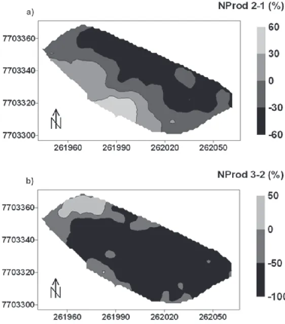
Considering the algebraic operation of the maps between the conilon coffee harvests, we determined the productivity levels (Nprod) between the different harvests, as shown in Figure 3.
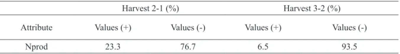
For better visualization and description of the results, the areas with positive and negative values were quantified as a percentage (%), indicating gain and loss areas in the maps (Table 1).
The analysis showed 76.7% for harvest 2-1 (Figure 3a), indicating a productivity inversion in the area between these harvests. Thus, the areas with lower altitudes in harvest 1 showed higher productivity. For harvest 3-2, the Nprod3-2 (Figure 3b) most of the area also showed negative values, concentrated in intervals from -50 to -100% of productivity reduction compared with the previous year, in the central part of the area.
The maps demonstrate positive and negative variability of productivity in different regions and between different harvests, indicating higher and lower productivity compared with previous harvests. This analysis allows visualizing regions that did not maintain the same productivity level from one harvest to another. Oliveira et al. (2010) showed that the mapping of the nutritional status of conilon coffee plants allowed visualizing different regions in the cultivation area, providing differentiated criteria for soil and leaf fertilization.
The interpretation of a harvest map for future localized management should take into account the consistent sources of variation, since there is hardly any control over transitory factors (QUEIROZ et al., 2004).
It is also known that in years of high load and high production in the coffee crop, there is a depletion of the plant in the next harvest. This is related to the fact that the plant is not able to balance the stages of fruit development and vegetative growth in its phenological cycle, and thus, may lead to reduced productivity.
Precipitation is another factor that may be related to the reduced productivity in the study area, since it influences the phenological stages of the coffee plant cycle. Damatta et al. (2007) worked with growth and development aspects of the coffee crop and found that two reproductive stages of the coffee plant can be affected by the occurrence of droughts: the floral bud development and grain formation. The monthly rainfall during the different harvests is shown in Table 2.
Bud development occurs between May and August.
TABLE 1 - Percentage of positive and negative values in the productivity maps (Nprod) between different harvests.
Harvest 2-1 (%) Harvest 3-2 (%)
Attribute Values (+) Values (-) Values (+) Values (-)
Nprod 23.3 76.7 6.5 93.5
Nprod: productivity levels
Higher precipitation was observed in May for harvest 2, June for harvest 2, July for harvest 1 and August for harvest 1. In the first two harvests, precipitation was higher and better distributed in the months of floral bud development (May-August, harvests 1 and 2), when compared to harvest 3 (May-August harvest 3). This indicates that in the third harvest, this fact may have influenced the development of flower buds and consequently, productivity. According to Berlato, Farenzena and Fontana (2005), climate instability will strongly influence the temporal variability of crop productivitys.
In the coffee plant, flower bud development has been related to moderate internal water deficit and climatic factors such as temperature, photoperiod and water availability, which are directly related to floral induction (THOMAZIELLO; OLIVEIRA; TOLEDO FILHO, 1997).
The temporal variability observed between the harvests may be related to several factors as the ones we have mentioned. However, Ferrão et al. (2007) have stated that the productive branches (orthotropic and plagiotropic) suffer from aging (depletion) after a number of harvests, with low production rates. This may also contribute to obstruct sunlight passage into the plant, which also reflects reduced production.
Therefore, among the current practices used for crop management of the conilon coffee, pruning is one of the most important, eliminating old and unproductive branches (orthotropic and plagiotropic) and restoring the balance between leaf area and total dry mass of the plant (DAMATTA et al., 2007).
After the determination of Nprod between harvests 2-1 and 3-2, the different class levels were weighed according to the respective occupied areas. Productivity indexes were then determined (YI), with YI2-1 of -18 % and YI3-2 of -57.1 %, providing from the methodology of spatial and temporal analysis a new vision in reduced productivity between the harvests.
The presence of lower productivity levels in the Nprod 3-2 map (-50 to -100%) explains the lower productivity index (YI3-2). There was a productivity reduction greater than 50.0% in harvest 3 when compared with harvest 2.
Productivity maps will be useful only to the extent that the information on intrinsic field factors can be correlated. However, in this study we did not seek to define a cause and effect relationship between various factors and productivity. Rather we have worked on a methodology to determine a loss and gain index between the harvests, considering the spatial and temporal dependence.
Therefore, mainly in the coffee crop, it is not simple to establish comparisons of productivity between the harvests, since it depends on the biennality, cultivar, cultural practices, soil fertility, planting density and weather conditions, all of which vary from year to year (SILVA; TEODORO; MELO, 2008).
4 CONCLUSION
1. The productivity in the three harvests has spatial and temporal variability.
2. Quantitative analysis using maps allows the observation that the productivity levels show alternate loss and gain regions between the different harvests.
3. The use of the map algebra methodology, which considers the spatial and temporal distribution in the studied area, allowed the determination of productivity reduction indices between the different harvests, providing the following values: -18% between the second and first harvest and of -57% between the third and second harvest.
5 AKNOWLEDGEMENTS
The authors thank the financial support by FAPES and CNPq in the development of this research.
TABLE 2 - Monthly rainfall (mm) during the three harvests of canephora coffee.
Harvest Aug Set Oct Nov Dec Jan Feb Mar Apr May Jun Jul
254 264 256 89 28* 35* 71*
1 45* 61 90 126 361 174 291 397 33 126** 68** 33**
2 22** 101 37 241 218 44 134 287 125 14*** 13*** 4***
3 10*** 78 67 267 198 237 100 62 46 25 19 7
*, **, *** Bud development of the first, second and third harvest, respectively.
6 REFERENCES
BARBOSA, D. H. et al. Estabelecimento de normas DRIS e diagnóstico nutricional do cafeeiro arábica na região noroeste do Estado do Rio de Janeiro. Ciência Rural, Santa Maria, v. 36, n. 6, p. 1717-1722, nov./dez. 2006.
BERLATO, M. A.; FARENZENA, H.; FONTANA, D. C. Associação entre El Nino Oscilação Sul e a produtividade do milho no Estado do Rio Grande do Sul. Pesquisa Agropecuária Brasileira, Brasília, v. 40, n. 5, p. 423-432, maio 2005.
CAMBARDELLA, C. A. et al. Field-scale variability of soil properties in Central Iowa soils. Soil Science
Society America Journal, Madison, v. 58, p.
1501-1511, 1994.
CARVALHO, L. G. et al. A regression model to predict coffee productivity in Southern Minas Gerais, Brazil. Revista Brasileira de Engenharia Agrícola e Ambiental, Campina Grande, v. 8, n. 2/3, p. 204-211, 2004.
DAMATTA, F. M. et al. Ecophysiology of coffee growth and production. Brazilian Journal of Plant Physiology, Piracicaba, v. 19, n. 4, p. 485-510, 2007. FERRÃO, R. G. et al. Café Conilon. Vitória: INCAPER, 2007. 702 p.
FERRAZ, G. A. S. et al. Agricultura de precisão no estudo de atributos químicos do solo e da produtividade de lavoura cafeeira. Coffee Science, Lavras, v. 7, n. 1, p. 59-67, 2012.
GOMES, F. P. Curso de estatística experimental. 12. ed. Piracicaba: Nobel, 1987.
GREGO, C. R.; VIEIRA, S. R. Variabilidade espacial de propriedades físicas de solo em uma parcela experimental. Revista Brasileira de Ciência do Solo, Viçosa, v. 29, n. 2, p. 169-177, 2005.
RENA, A. B. et al. Fisiologia do cafeeiro em plantios adensados. In: SIMPÓSIO INTERNACIONAL SOBRE CAFÉ ADENSADO, 1., 1996, Londrina. Anais... Londrina: Instituto Agronômico do Paraná, 1996. p. 73-85.
SILVA, C. A.; TEODORO, R. E. F.; MELO, B. Produtividade e rendimento do cafeeiro submetido a lâminas de irrigação. Pesquisa Agropecuária Brasileira, Brasília, v. 43, n. 3, p. 387-394, mar. 2008. SILVA, F. M. et al. Spatial variability of chemical attributes and productivity in the coffee cultivation. Ciência Rural, Santa Maria, v. 37, n. 2, p. 401-497, mar./abr. 2007.
SILVA, S. A. et al. Lógica fuzzy na avaliação da fertilidade do solo e produtividade do café conilon. Ciência Agronômica, Fortaleza, v. 41, n. 1, p. 9-17, 2010.
SILVA, S. A.; LIMA, J. S. S.; ALVES, A. I. Estudo espacial do rendimento de grãos e porcentagem de casca de duas variedades de coffea arabica l. visando a produção de café de qualidade. Bioscience Journal, Uberlândia, v. 26, n. 4, p. 558-565, 2010.
THOMAZIELLO, R. A.; OLIVEIRA, E. G.; TOLEDO FILHO, J. A. Cultura do café. 3. ed. Campinas: Instituto Agronômico, 1997. 75 p.
VIEIRA, S. R. et al. Spatial variability of soil chemical properties after coffee tree removal. Revista Brasileira de Ciências do Solo, Viçosa, v. 33, p. 1507-1514, 2009.
WEILL, M. A. M. et al. Avaliação de fatores edafoclimáticos e do manejo na produção de cafeeiros (Coffea arabica L.) no oeste Paulista. Revista Brasileira de Ciência do Solo, Viçosa, v. 23, n. 4, p. 891-901, 1999.
LIMA, J. S. S. et al. Métodos geoestatísticos no estudo da resistência do solo à penetração em trilha de tráfego de tratores na colheita de madeira. Revista Árvore, Viçosa, v. 32, n. 5, p. 931-938, 2008.
LIMA, J. S. S.; OLIVEIRA, R. B.; SILVA, S. A. Spatial variability of particle size fractions of an Oxisol cultivated with conilon coffee. Revista Ceres, Viçosa, v. 59, n. 6, p. 739-745, 2012.
LIMA, J. S. S.; SILVA, S. A.; SILVA, J. M. Variabilidade espacial de atributos químicos de um latossolo vermelho-amarelo cultivado em plantio direto. Ciência Agronômica, Fortaleza, v. 44, n. 1, p. 16-23, 2013. MILANI, L. et al. Unidades de manejo a partir de dados de produtividade. Acta Scientia Agronômica, Maringá, v. 28, n. 4, p. 591-598, 2006.
MIRANDA, N. O. et al. Variabilidade espacial da qualidade de frutos de melão em áreas fertirrigadas. Horticultura Brasileira, Brasília, v. 23, n. 2, p. 242-249, 2005.
MOLIN, J. P. Definição de unidades de manejo a partir de mapas de produtividade. Engenharia Agrícola, Jaboticabal, v. 22, n. 1, p. 83-92, 2002.
OLIVEIRA, R. B. et al. Spatial variability of the nutritional condition of canephora coffee aiming specific management. Coffee Science, Lavras, v. 5, n. 3, p. 190-196, 2010.
QUEIROZ, D. M. et al. Uso de técnicas de agricultura de precisão para a cafeicultura de montanha. In: ZAMBOLIM, A. (Ed.). Efeitos da irrigação sobre a qualidade e produtividade do café. Viçosa, MG: UFV, 2004. p. 77-108.