Prediction of dementia patients: A comparative approach using parametric vs. non parametric classifiers

Prediction of dementia patients: a comparative

approach using parametric vs. non parametric

classifiers

Jo˜ao Maroco, Dina Silva, Manuela Guerreiro, Alexandre de Mendonc¸a and Isabel Santana

Abstract In this paper, we report a comparison study of 7 non parametric classifiers (Multilayer perceptron Neural Networks, Radial Basis Function Neural Networks, Support Vector Machines, CART, CHAID and QUEST Classification trees and Ran-dom Forests) as compared to Linear Discriminant Analysis, Quadratic Discriminant Analysis and Logistic Regression tested in a real data application of mild cognitive impaired elderly patients conversion to dementia. When classification results are compared both on overall accuracy, specificity and sensitivity, Linear Discriminant Analysis and Random Forests rank first among all the classifiers.

1 Introduction

Traditional parametric statistical classification methods like Fisher’s Linear Dis-criminant Analysis (LDA) and Logistic Regression (LR) have been extensively used in the past in classification problems for which the criterion variable is dichotomous [1, 2, 3]. More recently, attention has been steadily building on the accuracy and efficiency of non parametric classifiers like Neural Networks (NN), Support Vector Machines (SVM), Classification Trees (CART) and Random Forests (RF) as ap-plied to classification problems [1, 4, 5, 6]. Research on the comparative accuracy for both parametric and non parametric methods has been growing steadily. Some authors defend that non parametric classifiers have higher accuracy and lower

er-Jo˜ao Maroco

Unidade de Psicologia e Sa´ude, & Departamento de Estat´ıstica. ISPA-Instituto Universit´ario, Rua Jardim do Tabaco, 34. 1149-041 Lisboa

e-mail:[email protected]

Dina Silva,Manuela Guerreiro, Alexandre de Mendonc¸a Instituto de Medicina Molecular, Universidade de Lisboa Isabel Santana

Servic¸o de Neurologia, Hospitais da Universidade de Coimbra

ror rates than the traditional parametric methods [7, 8, 9]. However, this superiority is not apparent with all data sets, especially with real data [10, 11, 12, 13, 14]. Results regarding classification accuracy and stability of the findings are still con-troversial [6, 15]. Most comparisons are based only on total classification accuracy and/or error rates; they involve human intervention for training and optimization of the non parametric classifiers vs. out-of-the-box results for the parametric classi-fiers. Accordingly to Duin [16] “(. . . ) a straight forward fair comparison demands automatic classifiers with no user interaction”. It also requires a large base compar-ison taking into account not only total accuracy but also sensitivity, specificity and discriminant power. Having prevented inadequate parametrizations of non paramet-ric classifiers, we compared total accuracy, sensitivity and specificity of traditional parametric classifiers (LDA, Quadratic Discriminant Analysis (QDA), LR) vs. non parametric methods derived from Data Mining and Machine Learning (NN, SVM, CART, RF). These methods were used to predict the evolution into dementia of 383 elderly people with mild cognitive impairment from several neuropsycholog-ical tests with predictive validity. When sensitivity and specificity were taken into account along with total classification accuracy, LDA reveals itself, with Random Forests, as one of the best classifiers. It is worthwhile to mention that LDA, a classi-fier devised ca. 100 years ago, still resists the challenges of the new classiclassi-fiers who required large computing power and user intervention.

2 Classifiers

2.1 Discriminant analysis

Fisher’s Linear Discriminant Analysis (LDA) estimates discriminant functions scores (D) for each of n subjects classified into k groups from p linearly independent pre-dictor variables (Xp) as

Dj= wj1X1+ wj2X2+ ... + wj pXp (1)

where j=1,. . . ,min(k-1,p). Discriminant weights (wj) are estimated by ordinary least squares so that the ratio of the variance within the k groups to the variance between the k groups is minimal. Classification functions of the type

Cj= cjo+ cj1X1+ cj2X2+ ... + cj pXp (2)

for each of the j=1,. . . ,k groups can be constructed. The coefficients of the clas-sification function for the j group are estimated from the within sum of squares matrices (W) of the discriminant scores for each group and from the means of the p discriminant predictors in each of the classifying groups (M) as Cj = W−1M with cjo= log p −1/2CjMj. Quadratic Discriminant Analysis (QDA) uses the same within vs. between groups sum of square minimization optimization but on a quadratic form discriminant function:

Dj= P

∑

∑

∑

with classification functions

Cj= c0 j+ P

∑

∑

∑

Both on LDA and QDA, a subject is classified into the group for which its classifi-cation function score is higher.

2.2 Logistic regression

Logistic regression (LR) models the probability of occurrence of one (success) of the two classes of a dichotomous criterion. A Logit transformation of the proba-bility of success for each subject (πi) is iteratively fitted to a linear combination of predictors accordingly to the model

Ln[ ˆπi/(1 − ˆπi)] =βo+β1X1i+β2X2i+ ... +βpXpi (5) by means of maximum likelihood estimation. Probability of success for each subject is estimated with the Logit model, and if the estimated probability is greater than 0.5 (or other pre-defined threshold value), the subject is classified in the success group; otherwise, it is classified into the failure group.

2.3 Neural networks

Neural Networks (NN) methods have been used in classification problems and this is one of the most active research and application areas in the Neural Networks field. A NN is a multi-stage, multi-unit classifier, with input, hidden or processing, and output layers. For a binary criterion ykthe NN can be described by the general model ˆ yk= fk(x, w, o, x0, o0k) = f h

∑

∑

where x is the vector of predictors, w is the vector of input weights, o is the vector of hidden weights, x0 and o0k are bias constants and h(.) and f (.) are activation functions for the hidden layer and output layer respectively. Activation functions are one of the general linear, logistic, exponential or Gaussian function families. Several topologies of Neural Networks (NN) can be used in binary classification

problems. Two of the most used NN are the Multilayer Perceptron (MLP) and the Radial Basis Function (RBF). The main differences between the two NN reside in the activation function of the hidden layer which belongs to the linear family in the MLP and to the Gaussian family in the RBF function. A NN is generally trained in a set of iterations (epochs) for a subset of the data (train set) and tested for the remained subset (test set). Synaptic weights of the NN are upgraded in each iteration in way to maximize the correct classification rate and/or minimize a function of the classification errors (for a detailed description of NN see [17]).

2.4 Support vector machines

Support Vector Machines (SVM) are machine-learning derived classifiers which map a vector of predictors into a higher dimensional linear plane through both lin-ear and non-linlin-ear kernelφ functions. In a binary classification problem, the two groups, say _{{-1} and {+1}, are then separated by a higher-dimension hyperplane} w′φ(x) + b = 0 where x is the vector of predictors, w is the weight vector and b is a

bias offset. The classification function is then

f(x) = Sign(w′φ(x) + b) (7) To find the optimum plane for both_{{-1} and {+1} groups, one strategy is to} maxi-mize the distance or margin of separation from the supporting planes, respectively w′φ_{(x)+ b ≥ +1 for the {+1} group and w}′φ_{(x)+ b ≤ −1 for the {-1} group. These} support planes are pushed apart until they bum into a small number of observations called ”support vectors”. This is equivalent to minimize a cost function

C(w) =kwk 2 2 + c n

∑

∑

under the constraints yi(w′φ(xi) + b) ≥ 1 −ξi and ξi≥ 0 where c>0 is penalty parameter for classification errors and ξi is the penalty of a misclassified obser-vation. In classification problems the usual kernel functions are the linear kernel φ(xi, xj) = xi′xjand the Gaussianφ(xi, xj) = exp(−γ

xi− xj

2

) whereγis a ker-nel parameter (for a complete description of SVM see [7, 18]).

2.5 Classification trees

Classification Trees (CT) are non parametric classifiers that construct decision trees by splitting a node, accordingly to an “if-then criteria” applied to a set of predictors, into two child nodes repeatedly, from a root node that contains the whole sample. Thus, CT can select the predictors and its interactions that are most important in

de-termining an outcome for a criterion variable. The development of a CT is supported on three major elements: (1) choosing a sampling-spliting rule that defines the tree branch which connect the classification nodes; (2) the evaluation of the goodness of fit produced by the splitting rule at each node and (3) the criteria used for choos-ing an optimal or final tree for classification proposes. Accordchoos-ingly to the features of these major elements, CT can be classified into CART, CHAID and QUEST. In CART trees, the predictors are split (if they are continuous) or classes are separated (if they are qualitative) with the objective of reducing the impurity of the final node produced at each t branch of the tree. The Gini impurity index

IG(t) = 1 − C

∑

∑

∑

P_{(c|t) =}P(c,t) P(t) with P(c,t) = π(c)nc(t) nc and P(t) = C

∑

whereπ(c) is the probability of observing the group c and nc(t) is the number of elements in group c at a given node t. The tree grows until no further predictors can be used or the impurity of each group at the final branch of the tree can not be reduced further. Non significant branches can be pruned from the final tree. In CHAID trees, the homogeneity of the groups is evaluated by a Bonferroni corrected p-value from the Pearson chi-square statistic applied to two-way classification tables with C classes and K splits. In QUEST, the homogeneity of groups at each branch is evaluated with the ratio of the within group variance and between group variances for continuous predictors or a chi-square like statistic for categorical predictors. Although several other alternative algorithms are also available, in this study we only compared well established CART, CHAID and QUEST algorithms (see [19]).

2.6 Random forests

Random forests (RF) construct a series of CART using different bootstrap samples of the original data sample. Each of these CART trees is build from a random sub-set of the total predictors who maximize the classification criteria at each node. An estimate of the classification error-rate can be obtained using each of the CART to predict the data not in the bootstrap sample (“out-of-the bag”) used to grow the tree, and average the out-of-the bag predictions for the grown forest. These out-of-the bag estimates of the error-rate can be quite accurate if enough trees have been grown. Although this classification strategy may lack a perceivable advantage over single CART, accordingly to its creator (Leo Breiman [22]) it has unexcelled accuracy when compared to many classifiers including LDA, NN and SVM.

3 A classification application

3.1 Sample

The described classifiers were used to predict the conversion of 383 elderly patients with Mild Cognitive Impairment (MCI) to dementia (see Table 1 for sample demo-graphics).

Table 1 Sample demographicsa.

Groups MCI Dementia p-value

Size 262 (68%) 121 (32%) 0.001 ‡

Age (Mean_{± SD)} 68.3_±8.5 71.1_±8.6 0.003†

Sex (Male/Female) 157 / 103 75 / 46 0.822‡

Schooling years (Mean_{± SD)} 8.2_{± 4.7} 8.6_{± 5.0} 0.436† Time between assessments (year)(Mean_{± SD) 2.4 ± 1.6} 2.4_{± 1.7} 0.881†

a_{”MCI”- patients who remained in MCI; and ”Dementia”- patients who progressed to dementia.} p-values for group comparison were obtained from Student’s-t test (†) orχ2test(‡)

Thirty-two percent of participants showed dementia (the event to predict). Distri-butions of sex, schooling years and time between assessments did not differ signifi-cantly between the dementia vs. MCI groups. However, mean age was signifisignifi-cantly lower for the MCI group (p_{≤ 0.05).}

3.2 Criterion and predictors

The criterion was a dichotomous variable with two groups: MCI and Dementia. Predictors used to predict the conversion of MCI into dementia were a set of 9 quantitative neuropsychological tests which have previously shown criterion valid-ity (i.e. statistically significant different scores for the MCI vs. Dementia groups): Digit Span backward (evaluates working memory), the Logical Memory test (evalu-ates episodic memory), Verbal Paired Associ(evalu-ates Learning (evalu(evalu-ates learning abil-ity), Word Recall (evaluates short-term memory), Orientation (evaluates personal, spatial and temporal orientation), Semantic Fluency (evaluates verbal initiative), Clock Drawing (evaluates visual constructive abilities), the Raven Progressive Ma-trices (evaluates non-verbal abstract reasoning) and Proverbs test (evaluates verbal abstract reasoning). Figure 1 shows the scatter plot of these predictors and their fre-quency histograms. Predictors lack homogeneity of group variances and their his-tograms show several predictors with a considerable departure from the Gaussian distribution. There were also several outliers.

Fig. 1 Scatter plots for MCI (_{•) and Dementia (◦) patients in the 9 predictors and its histograms}

(DSB - Digit Span Backward test; SF - Semantic Fluency; Or - Orientation; WR - Word Recall; VPAL - Verbal paired association learning; LM - Learning Memory; Clock - Clock drawing; MPR - Raven Progressive Matrices; Prov - Proverbs)

3.3 Classification settings

A 5-fold cross-validation strategy was followed to train and evaluate all the clas-sifiers. The total sample was divided into 5 proportional sub-samples. In each of the 5 steps, 4/5 of the sample was used for training and 1/5 was used for testing. Test results for the 5 runs were then aggregated and the comparative performances of the different classifiers evaluated with Friedman’s ANOVA on Ranks followed by a multiple comparison on mean ranks. Statistical significance was assumed for p<0.05. Linear and Quadratic Discriminant Analysis and Logistic Regression used

equal a priori classification probabilities. Data was checked for univariate and mul-tivariate outliers. As far as the parametric assumptions of LDA (normality of predic-tors and homogeneity of group variances), no considerable deviation of normality for most predictors and no large differences between group variances were observed. As it is well known, LDA is quite robust to moderate violations of its assumptions. The MLP Neural Network was trained in a 80%:20% train:test setup, with 9 inputs, 1 hidden layer with 4-7 neurons and a hyperbolic tangent activation function. The activation function for the output layer was the Softmax with a cross-entropy error

function. The RBF Neural Network had 9 inputs, one hidden layer with 2-8 neurons and a Softmax activation function. The activation function for the output layer was the identity function with a sum of squares error function. The SVM kernel was the radial basis (Gaussian) function with cost (c) andγparameters optimized by a grid search in the intervals[2−3_{; 2}15_{] for c and [2}−15_{; 2}3_{] for}γ_{, followed by internal} 10-fold cross-validation. The classification function was the sign of the optimum margin of separation. Classification Trees used the CHAID, CART and QUEST al-gorithms, withα to split andαto merge of 0.05, with 10 intervals. Tree growth and pruning (for CART) was set with a minimum parent size of 5 and minimum child size of 1. Classification priors were 0.5:0.5. Random Forests were grown on 500 CART with 2-6 predictors per tree and tree optimization by cross-validation. Dis-criminant Analysis, Logistic Regression, Neural Networks and Classification trees were performed with PASW Statistics (v. 18, SPSS Inc., Chicago, Il). Support Vec-tor Machines and Random Forests were performed with R (v. 2.8, R Foundation for Statistical Computing, Vienna, Austria) with the e1071[20] and randomForest [21] packages respectively.

3.4 Results

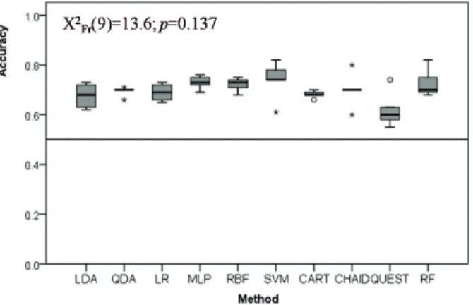
Classification accuracy, sensitivity and specificity were evaluated in the 5 test sets resulting from the 5-fold cross validation strategy. Data gathered are shown as box-plots for the different classifiers. Figure 2 shows the box-box-plots of the total classifica-tion accuracy for the 10 classifiers studied. When the distribuclassifica-tions of total accuracy are compared with the Friedman test, the observed differences were not statistically significant (X2_Fr(9)=13.6; p=0.137).

Fig. 2 Box-plot distributions of classification accuracy (number of correct classifications / total

sample size) for the 5 test samples resulting from the 5-fold cross-validation procedure (see text for abbreviations).

The distributions of specificity (that is the proportion of subjects that did not convert into dementia and were correctly predicted by the classifier) are shown in figure 3. There were statistical significant differences in the specificity distributions of the different classifiers X2

Fr(9)=34.868; p<0.001). SVM, MLP, LR and RF presented the highest specificity values which were significantly different from a second group composed by LDA, QDA and CART.

Fig. 3 Box-plot distributions of specificity (number of MCI predicted / number of MCI observed)

for the 5 test samples resulting from the 5-fold cross-validation procedure (see text for abbrevia-tions). Different letters indicate statistically significant differences between classifiers on a multiple mean rank comparison procedure.

Figure 4 shows the distributions of sensitivity (proportion of subjects that were cor-rectly predicted to convert into dementia). There were statistically significant dif-ferences in the distributions of sensitivity (X2_Fr(9)=37.9;p<0.001). LDA, CART,

QUEST and RF had the highest sensitivity values which were significantly different from a second group composed by LR, MLP, RBF and CHAID. It is worthwhile to mention that this second group had sensitivity lower than 0.5, and that SVM was the classifier with lowest sensitivity.

Fig. 4 Box-plot distributions of sensitivity (number of Dementia predicted / number of Dementia

observed) (see text for abbreviations). Different letters indicate statistically significant differences between classifiers on a multiple mean rank comparison procedure.

4 Discussion

Although no statistically significant differences were found in total accuracy of the 10 evaluated classifiers (Medians between 0.60 and 0.74), a quite different picture emerges from the analysis of specificity and sensitivity of the classifiers. Median specificity ranged from a minimum of 0.53 (QUEST) to a maximum of 1 (SVM). With the exception of QUEST, all the other classifiers were quite efficient in predict-ing group membership in the group with larger number of elements (the MCI group corresponding to 68% of the sample) (Median specificity larger than 0.6). However, predictions for the group with lower frequency (the Dementia group, correspond-ing to 32% of the sample) were quite unsatisfactory. Minimum median sensitivity was 0.14 (SVM) and maximum median sensitivity was 0.7 (LDA). Only five of the ten classifiers tested showed median sensitivity larger than 0.5. Conversion into de-mentia is the key prediction in this biomedical application, requiring classifiers with high sensitivity. Thus, on this real data example, classifiers like Logistic Regres-sion, Neural Networks, Support Vector Machines and CHAID trees are inappropri-ate for this binary classification task. Also, total accuracy of classifiers is misleading since some classifiers are good only at predicting the larger group membership (high specificity) but quite bad at predicting the smaller group memberships (low sensi-tivity). Some of the classifiers with the highest specificity (NN and SVM) were also the classifiers with the lowest sensitivity. Unbalance of classification efficiency for small frequency vs. large frequency groups has been found in other real-data stud-ies for logistic regression and Neural Networks [10, 23, 25, 24]. Taking in account both total accuracy, specificity and sensitivity, the oldest Fisher’s Linear Discrim-inant Analysis ranks top with Random Forests, the newest member of the binary classification family. Similar observations have been made by other authors. For example, Breinman et al. (1984) states that LDA does as well as other classifiers in most applications. Meyer et al. [24] point out in their comparison study of data mining classifiers, including NN and SVM, that LDA is a very competitive classi-fier, ”producing good results out-of-the-box without the inconvenience of delicate and computationally expensive hyperparameter tuning”. For simple binary classi-fication problems, where sample size may compromise training and testing of non parametric data mining and machine learning classifiers, Fisher’s Linear Discrimi-nant Analysis stands up as a simple, efficient and time-proof classifier.

References

1. Goss, E.P., Ramchandani, H.: Comparing classification accuracy of neural networks, binary logit regression and discriminant analysis for insolvency prediction of life insurers. J. Econ. Fin. 19(3):1–18 (1995)

2. Lei, P.W., Koehly, L.M.: Linear discriminant analysis versus logistic regression: a comparison of classification errors in the two-group case. J. Exp. Educ. 72(1), 25–49 (2003)

3. Pohar, M., Blas, M., Turk, S.: Comparison of Logistic Regression and Linear. Discriminant Analysis: A Simulation Study. Metodoloˇski zvezki 1(1), 143–161 (2004)

4. Pitarque, A., Roy, J.F., Ruiz, J.C.: Redes neurales vs modelos estad´ısticos: Simulaciones sobre tareas de predicci ´on y clasificaci ´on. Psicol ´ogica 19, 387–400

5. Nabney, I.T. (2004) Efficient training of RBF networks for classification. Int. J. Neural Syst. 14(3):201–208 (1998)

6. Sommer, M., Olbrich, A., Arendasy, M.:Improvements in Personnel Selection with Neural Nets: A Pilot Study in the field of Aviation Psychology. Int. J. Aviat. Psychol. 14(1), 103–115 (2004)

7. Ivanciuc, O.: Applications of Support Vector Machines in Chemistry. Reviews in Computa-tional Chemistry, eds Lipkowitz KB & Cundari TR (John Wiley & Sons, Inc, Weinheim),

23,291–400 (2007)

8. Sut, N., Senocak, M: Assessment of the performances of multilayer perceptron neural net-works in comparison with recurrent neural netnet-works and two statistical methods for diagnos-ing coronary artery disease. Expert Syst. 24(3),131–142 (2007)

9. Kurt, I., Ture, M., Kurum, A.T.: Comparing performances of logistic regression, classification and regression tree, and neural networks for predicting coronary artery disease. Expert Syst. Appl. 34(1),366–374 (2008)

10. Finch, H., Schneider, M.K.: Classification Accuracy of Neural Networks vs. Discriminant Analysis, Logistic Regression, and Classification and Regression Trees: Three- and Five-Group Cases. Methodology 3(2), 47–57 (2007)

11. Gelnarova, E., Safarik, L.: Comparison of three statistical classifiers on a prostate cancer data. Neural Network World 15(4):311–318 (2005)

12. Green, M., Bj ¨ork, J., Forberg, J., Ekelund, U., Edenbrandt, L., Ohlsson, M.: Comparison between neural networks and multiple logistic regression to predict acute coronary syndrome in the emergency room. Artif. Intel. Med. 38(3):305–318 (2006)

13. Paulo, J.L.A., Vasconcelos, G.C., Arnaud, A.L., Santos, R.A.F., Cunha, R.C.L.V., Monteiro, D.S.M.P.: Neural Networks vs Logistic Regression: a Comparative Study on a Large Data Set. 17th International Conference on Pattern Recognition (ICPR’04) 3,355–358 (2004) 14. Peter, C.A.: A comparison of regression trees, logistic regression, generalized additive

mod-els, and multivariate adaptive regression splines for predicting AMI mortality. Stat. Med.

26(15),2937–2957 (2007)

15. Ghaffari, M., Hall, E.L.: Experimental approach for the evaluation of neural network classi-fier algorithms. Intelligent Robots and Computer Vision XXI: Algorithms, Techniques, and Active Vision., eds Casasent DP, Hall EL, & R¨oning J ( SPIE Bellingham WA ) 5267,250–256 (2003)

16. Duin, R. P. W.: A note on comparing classifiers. Pattern Recog. Lett. 17(5),529–536 (1996) 17. Bishop, C.: Neural Networks for Pattern Recognition, Oxford University Press, Oxford (1995) 18. Bennett, K.P., Campbell, C.: Support vector machines: Hype or hallelujah? SIGKDD Expl.

2(2), 1–13 (2000)

19. Breiman, L., Friedman, J.H., Olshen, R.A., Stone, C.J.: Classification and regression trees. Wadsworth, Inc, Monterey, Calif., U.S.A. (1984)

20. Meyer, D.: Support Vector Machines: The Interface to libsvm in package e1071. R News

1/3:23–26 (2001)

21. Liaw, A., Wiener, M.: Classification and Regression by randomForest. R News

2/3(December):18–22 (2002)

22. Breiman, L.: Random Forests. Machine Learning 45(1):5–32 (2001)

23. Schwarzer, G., Vach, W. & Schumacher, M.: On the misuses of artificial neural networks for prognostic and diagnostic classification in oncology. Stat. Med. 19(4):541–561 (2000) 24. Meyer, D., Leischa, F., Hornik, K.: The support vector machine under test. Neurocomputing

55(1-2):169–186 (2003)

25. Maroco, J., Bartolo-Ribeiro, R.: M´etodos de classificac¸˜ao bin´aria no contexto da selecc¸˜ao de pilotos militares. Comparac¸˜ao da precis˜ao classificat ´oria de Redes Neuronais, Regress˜ao Log´ıstica e An´alise Discriminante Linear. XV Congresso da Sociedade Portuguesa de Es-tat´ıstica, ed Hill M et al (SPE), 289–304 (2008)