Optimizing the number of progenies and replications in plant
breeding experiments
João Luís da Silva Filho1*
Received 05 June 2012
Accepted 19 August 2013
Abstract – A determination criterion was proposed for the number of replications, r, and of evaluated progenies, Nr, given P experi-mental plots, with Nr=P/r, and n progenies to be selected; its application was discussed in the selection of progenies of bulk popula-tions, derived from two homozygous parents. For a known heritability at the plot level, h2
0, there is a critical n below which the gain is greater with selection evaluating P/(r+1) progenies in r+1 than P/r progenies in r replications. Different h2
0 scenarios were simulated in the F2 and F∞ generations, assuming no dominance. It was demonstrated that at any h2
0 , if n > 18.5% of P, larger gains are obtained by assuming Nr = P, showing that the augmented block design could be used in the early stages of breeding programs. The higher h2
0, the higher must be the selection intensity to justify the use of additional replications.
Key words: Selection gains, population sample size, number of selected progenies, selection limits. INTRODUCTION
In plant breeding, due to limitations in the experimental area or available resources, it is impossible to evaluate experiments with the number of replications and number of progenies desirable for breeders. In the process of developing inbred lines, be it for cultivars or as hybrid parents, a limited number of progenies may undermine the representativeness of genetic variability, whereas a small number of replications can compromise the experimental accuracy. Both situations contribute to reduce genetic gain with selection (GS).
To overcome this problem, considerable research ef-fort has been invested, to identify the best way to manage, sample and/or evaluate segregating populations, with previ-ously available experimental results for some crops. In the case of common bean, for example, success with selection in biparental crossings can be obtained by any method of population management, although due to operational ease
and flexibility, the population (or bulk) and single seed
descent (SSD) method are most advantageous (Raposo et al. 2000). In addition, at least 100 progenies should be evaluated to represent the genetic variability of a population satisfactorily and to ensure successful selection, according to the experimental conditions of breeding programs (Fer-reira et al. 2000).
The number of replications and/or, the ideal plot size to estimate genetic parameters or compare progenies and/or cultivars, were also investigated and satisfactorily determined,
varying with the crop and trait considered (Storck et al.
2007, Vieira and Silva 2008, Leite et al. 2009, Cargnelutti
Filho et al. 2010, Silva et al. 2011, Storck et al. 2011 and
Cargnelutti Filho et al. 2012).
Another aspect is the difficulty of measuring the ac
-curacy of a test appropriately, since the efficiency of the experimental coefficient of variation, the most widely used
criterion, is questionable, and the use of selective accuracy is preferable (Resende and Duarte 2007).
In fact, the interest of breeders is to maximize the GS and according to Kempton and Fox (1997), it is necessary to consider: i) the number and choice of parental crosses, ii) the number of replications per experiment and the number of evaluated locations, the size of the improvement program and the proportion of progenies selected at each stage. These authors mention the constant doubt, whether screening a large number of progenies or a more accurate evaluation with fewer progenies using more replications should be preferred. They claim that two or three replications can be used, when enough seeds are available.
When the experimental area is limited, the use of more replications implies in a reduction of the number of progenies. Crop Breeding and Applied Biotechnology 13: 151-157 2013
Brazilian Society of Plant Breeding. Printed in Brazil
ARTICLE
1 Embrapa Arroz e Feijão - Núcleo do Algodão do Cerrado, Rodovia GO-462, km 12, CP 179, 75.375-000, Santo Antônio de Goiás, GO, Brazil.
From the GS equation, Bos and Caligari (2008) compared gains by selection using one or more than one observation
per progeny, with a fixed number of plots and of selected
progenies. The authors show that it is not always advanta-geous to increase the number of replications instead of the number of evaluated progenies.
In breeding programs, frequently a number of progenies to be selected has to be determined, especially in the early stages. This number must not be so large that the
instal-lation of a test network would become unfeasible, nor so
small that studies of genotype x environment interaction and cultivar recommendation for different environments would be affected.
In this study the idea proposed by Bos and Caligari (2008) was extended to decisions between the assessment of P/r progenies with r replications or P/(r+1) progenies with r+1 replications, which varies according to the
heri-tability at the plot level. The selection of progenies taken from bulk populations, derived from biparental crosses of
homozygous parents was discussed, considering no domi-nance, although, theoretically, the criterion could be applied to other breeding strategies.
MATERIAL AND METHODS
Theory
Let P be plots available, Nr progenies with r replications, such that P = Nr ∙ r, and n the number of selected progenies. Hence, if r = 1, then Nr = P, and the percentage of truncated selection, t, is given by: . For any r:
Then, for each replication being additionally included in the experiment, maintaining P plots:
When n is constant, t(r+1) > t(r). Thus, the ratio between t(r+1) and t(r) is given by:
If the progeny effects are random, the narrow-sense heritability at the plot level is:
where σ2
a is the additive genetic variation and σ 2
e the residual variance. Assuming the denominator of equation (6) as 1, then: h2
0 = σ 2 a and σ
2 e = 1 – h
2
0 . In experiments with r replica-tions, the heritability (h2
0) and phenotypic standard deviation (σr) in the mean of observations are given by:
From the equation of GS, using standard deviations i, the use of r2 replications instead of r1, for r2 > r1, must satisfy the condition GS2 > GS1 to be beneficial:
i2h2 2σ2 > i1h
2 1σ1
If n corresponds to a percentage t(r) when r replications
are used, is the percentage of selection when
r+1 replications are used, are the
respective values of the standardized selection intensities and di(t) the critical ratio between them. Assuming r1 = r and
Then, there is a critical value for n, nc(r), below which
GS is larger when r+1 replications are used and N(r+1) progenies instead of r replicates and Nr progenies, which can be determined by choosing two critical selection percentages, tc(r) and tc(r+1), which satisfy the values dt(r) (5) and di(t) (10).
Let, for example, nc(r) be determined in a way that the use of two replications, r +1 = 2, is advantageous for a single observation, r = 1; then, dt(r) = 2 and
. For illustration, assuming a very
low h2
0, tending to zero, di(t) = 0.707. The two selection ratios that meet dt(r) = 2 and di(t) = 0.707 were 18.5% (it(r) = i18.5.% = 1.443) and 37.0 % (i2t(r) = i37% =1.020). Thus, tc(r) = 18.5% and tc(r+1) = 37.0% and . So, theoretically, for
n > 18.5% of P, gains are larger when an increase in the number of progenies is prioritized, Nr = P, even when h2
0 is low.
Simulation
An availability of 600 experimental plots was taken
into consideration and the following arrangements were compared: a) Nr = 600 progenies and r = 1 vs. N(r+1) = 300 progenies r+1 = 2; b) Nr = 300 and r = 2 vs. N(r+1) = 200 and r+1 = 3; c) Nr = 200 and r = 3 vs. N(r+1) = 150 for r+1 = 4. Equation (9) can be used for any two replications r1 and r2. However, in this article, only consequences of the decision to use a single additional replication are pointed out (Equation 10).
The purpose was to validate by simulation, at different
h2
0 levels, whether nc(r) is a good criterion to decide about using r or r +1 replications for Nr and N(r+1) evaluated progenies, respectively, given the selection objective of n
progenies. Simulations with nc(r), nc(r) + 2% ∙ Nr and nc(r)
– 2% ∙ Nr selected progenies were performed. If nc(r) is a good criterion, it is expected that GS for nc(r) + 2% ∙ Nr is greater in a scenario with Nr and r and the GS for nc(r) – 2%
∙ Nr would be greater with Nr+1 and r+1. In the selection of
ncr progenies, similar GS are expected in both situations.
Three levels of h2
0 (0.2, 0.35, 0.50) were simulated
using SAS/IML software. A bulk base population was
considered, derived from a cross between contrasting homozygous parents without dominance and 50 genes controlling the trait, independent and with equal value and plants sampled in the F2 (F2:3 progenies) and F∞, generation (homozygous lines). Favorable homozygotes
(AA) were assigned value 1 and unfavorable homozygous (aa) -1, while heterozygotes (Aa) were assigned 0. In the F2 generation, the heterozygous genotype frequency was assumed as 0.5 and homozygote frequency as 0.25. In F∞, 0.5 was assumed as genotypic frequency value of homozygotes. The parametric value of the progenies was assumed to be the arithmetic sum of the values of the 50 loci. Under the simulated conditions, the genetic variance in F2 is 25 and 50 in F∞,. Per plot and simulation, a random number was generated from a normal standard distribution, later multiplied by the value of the residual standard deviation, corresponding to the simulated h2
0, which is the residual plot value. The phenotypic value of each observation was assumed as the sum of the parametric value of the progeny plus the sum of the residual plot value. Estimates of GS were obtained by subtracting the parametric mean of the population from the parametric mean of the selected progenies based on phenotypic values, considering an average of 2000 simulations for each scenario considered for inferences. The mean standard error of GS was also calculated from the values of the 2000 simulations.
Example of a comparison procedure
600 plots (P = 600);
Compare: 300 progenies with two replications and 200 with three, and h2
0 = 0.2;
In this case, using Equation 10 with r = 2, r+1 = 3, we have:
The two selection proportions that simultaneously satisfy dt(r) = 1.5 and di(t) = 0.882 are 10.6 % and 15.9%. So, tc(r) = 10.6%, and nc(r) = tc(r) ∙ (P / r) = 0.106 x 300 = 31. If the parametric nc(r) is really close to 31, it is expected that the GS of 37 progenies (31 + 2% of 300) is higher when 300 progenies are evaluated with two replications and the GS of 25 progenies (31 - 2% of 300) is greater than 200 when evaluated with three replications.
RESULTS AND DISCUSSION
Critical selection proportions for different heritability levels
The values of di(t) and the corresponding tc(r) and tc(r+1)
were contrasted in five comparisons of the use of an
additional replication, at different levels of h2
0 (Table 1), in other words: 1 replication vs. two, two vs. three, three
vs. four, four vs. five five vs. six replications. Deciding
of selected progenies, is the GS larger when sampling the population to the limit of available plots, with a single observation per progeny, or when using half the sample size, but with two observations per progeny, improving the experimental accuracy of selection?
If the chosen strategy is screening or pre-breeding selection, the use of many replications is unnecessary, even when h2
0 is low. As a rule, the higher h 2
0, the more intense selection has to be to justify the use of additional replications. For a given h2
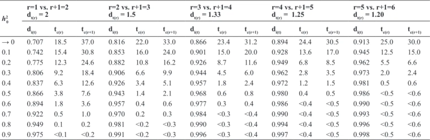
0, nc(r) can be obtained by making nc(r) = tc(r) ∙ (P / r). If h2
0, = 0.1, r = 1 and r+1 = 2, the values of tc(r) and tc(r+1) are, respectively, 15.4% and 30.8%, for any desired n, if n / Nr < 15.4 % (or n / Nr+1 < 30.8%), then,
GS for Nr+1 > GS with Nr, preferably evaluating Nr+1 in r+1 replications.
Our results are consistent with those presented by Bos and Caligari (2008). Assuming h2
0 = 0.5, it was observed that gains for r +1 = 2 were only superior to r = 1 if tc(r) < 3.8% (Table 1). For h2
0 = 0.5 and v ≥ 4% (v = n/P in Bos and Caligari (2008)), higher gains were obtained with one observation than with two (vj for J=2 in the said study); when v ≤ 3%, higher gains were obtained with
two replications. Similarly, when r=1, r+1=2 and h2 0 ≤ 0.4, the use of two replications is advantageous, provided that the selection intensity is < 6.3%, as also reported by Bos and Caligari (2008). In the table presented by these authors, at h2
0 ≤ 0.4, the gains with vj, for J=2 were always
greater than with a single observation per progeny for all v values (0.5%, 1%, 2%, 3%, 4%, 5%, or 6%). The advantage of the table presented here is to directly provide the selection ratio limit to decide on whether to
use Nr or Nr+1 progenies, facilitating decision making. The use of two or three replications suggested by Kemp-ton and Fox (1997) was also corroborated by the data (see Table 1). Assuming h2
0 = 0.2, the use of four replications r +1 = 4, or instead of three, r = 3, would only be advanta-geous if n / Nr < 8.7% (or n / Nr+1 < 11.6).
Summaries of sampling information (P, r and r+1, Nr and Nr+1, h2
0 , h 2 r and h
2
r+1) and theoretical critical values (dt(r), di(t), tc(r) and tc(r+1), nc(r)) for each of the simulated comparisons are shown in Table 2. Assuming 600 plots (P = 600) and selection of 30 progenies (n = 30), would it be more advantageous to choose 30 among 600 progenies, with a single observation (5% selection), or choose 30 of 300 (10% selection), but evaluated with two replications?
It was shown that if h2
0 = 0.35: h 2
r = 0.35 (heritability of 600 evaluated progenies r = 1), h2
r+1 = 0.519 (heritability
of 300 progenies r+1 = 2); tc(r) = 7.6 % and tc(r+1) = 15.2 % and nc(r) = 0.076 x 600 = 45. Since 30 < nc(r), it would be convenient to select 30 out of 300, because the gain in ac-curacy compensates the lower selection intensity. If h2
0 = 0.5, h2
r = 0.5, h 2
r+1 = 0.667; tc(r) = 3.7 % and tc(r+1) = 7.4 %, nc(r) = 22, then it is best to select 30 among 600 because, in this case 30 > ncr.
For models in which the random effects are only prog-enies and the experimental error of the selective accuracy is the square root of heritability at the mean progeny level (Equation 7); in the case of other random effects in the model,
the selective accuracy is influenced by the magnitude of the
variances of these effects. Further details are given by Mrode (2005). In these examples, a small variation in heritability
(0.15) modified the choice of the experimental strategy.
Therefore, the more accurate the heritability estimates, the more reliable is the proposed criterion.
Table 1. Critical ratios between standardized selection intensities (di(t)) and critical percentages of selection for the use of r or r+1 replications (tc(r) and
tc(r+1)), at different heritabilities at the plot level (h 2
0), in five comparisons using an additional replication: r = 1 vs. r+1 = 2; r = 2 vs. r+1 = 3, r = 3 vs.
r+1 = 4, r = 4 vs. r+1 = 5 and r = 5 vs. r+1 = 6
h2 0
r=1 vs. r+1=2 dt(r) = 2
r=2 vs. r+1=3 dt(r) = 1.5
r=3 vs. r+1=4 dt(r) = 1.33
r=4 vs. r+1=5 dt(r) = 1.25
r=5 vs. r+1=6 dt(r) = 1.20
di(t) tc(r) tc(r+1) di(t) tc(r) tc(r+1) di(t) tc(r) tc(r+1) di(t) tc(r) tc(r+1) di(t) tc(r) tc(r+1)
→ 0 0.707 18.5 37.0 0.816 22.0 33.0 0.866 23.4 31.2 0.894 24.4 30.5 0.913 25.0 30.0 0.1 0.742 15.4 30.8 0.853 16.0 24.0 0.901 15.0 20.0 0.928 13.6 17.0 0.945 12.5 15.0 0.2 0.775 12.3 24.6 0.882 10.8 16.2 0.926 8.7 11.6 0.949 6.8 8.5 0.962 5.5 6.6
0.3 0.806 9.2 18.4 0.906 6.6 9.9 0.944 4.5 6.0 0.962 2.8 3.5 0.973 2.0 2.4
0.4 0.837 6.3 12.6 0.926 3.4 5.1 0.957 1.8 2.4 0.972 1.2 1.5 0.981 0.5 0.6
The comparisons of 300 (r = 2) versus 200 (r+1 = 3) were performed for h2
0 = 0.2 and 0.35 and for 200 (r = 3) versus 150 (r +1 = 4) only for h2
0 = 0.2, since it was theoreti-cally expected that a number of plots well over 600 would be required for safe simulations of the comparisons, since tc(r) was very low.
RESULTS OF SIMULATIONS
The results for different scenarios of h2
0, n and Nr (600, 300, 200, 150, with r replications) are shown in Table 3. As
expected, in the same Nr, type of population and h2 0 , larger GS was obtained with greater selection intensity (lower n values). A positive effect on GS of the increase in h2
0, under the same selection intensity, was also observed. For 600 or 300 evaluated plants, the GS with n = 34, when h2
0 = 0.5, was higher than GS with n = 33, when h2
0 = 0.35.
There was perfect correlation between the results of simulations and the nc(r) determined by the criteria described (represented by “*” in Table 3). Comparing the GS of Nr with Nr+1, at any h2
0 in the F2 or F∞ populations, it was shown
Table 2. Number of plots (P), number of evaluated progenies (Nr and Nr+1) with r and r+1 replications, heritability at the plot level (h2
0), and the
prog-eny mean in Nr (h 2
r) and Nr+1 (h 2
r+1 ), critical selection percentages in Nr and Nr+1 (tc(r) and tc(r+1)), the ratio between tc(r) and tc(r+1) (dt(r)), the ratio between
the intensities of standardized selection of tc(r) and tc(r+1) (di(t)), the critical value of the number of selected progenies using r replications (nc(r)) for the different simulated scenarios
P Nr Nr+1 R r+1 h
2
0 h
2
r h
2
r+1 dt(r) di(t) tc(r) tc(r+1) nc(r)
600 600 300 1 2 0.20 0.200 0.333 2.00 0.775 12.2 24.4 73
600 600 300 1 2 0.35 0.350 0.519 2.00 0.822 7.6 15.2 45
600 600 300 1 2 0.50 0.500 0.667 2.00 0.866 3.7 7.4 22
600 300 200 2 3 0.20 0.333 0.429 1.50 0.882 10.6 15.9 31
600 300 200 2 3 0.35 0.519 0.618 1.50 0.916 4.8 7.2 14
600 300 200 2 3 0.50 0.667 0.750 1.50 0.943 1.4 2.1 4
600 200 150 3 4 0.20 0.429 0.500 1.33 0.926 8.4 11.2 16
600 200 150 3 4 0.35 0.618 0.683 1.33 0.951 2.7 3.6 5
600 200 150 3 4 0.50 0.750 0.800 1.33 0.968 0.6 0.8 1
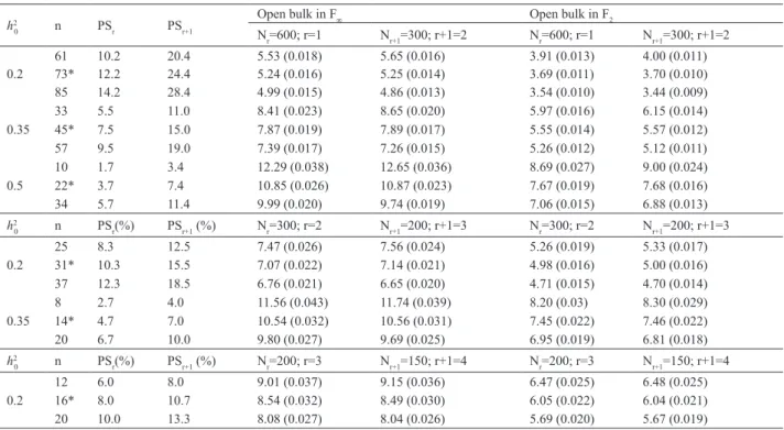
Table 3. Selection gains and their standard errors (in parentheses) obtained for open bulk in F2 and F∞ generation, at different heritabilities at the plot
level (h2
0), number of selected progenies (n), selection percentage when r (PSr) and r+1 (PSr+1) replications are used and number of evaluated progenies
with r (Nr) and r+1 (Nr+1) replications, assuming 50 genes controlling the character, allele frequency of 0.5 and absence of dominance
h2
0 n PSr PSr+1
Open bulk in F∞ Open bulk in F2
Nr=600; r=1 Nr+1=300; r+1=2 Nr=600; r=1 Nr+1=300; r+1=2
61 10.2 20.4 5.53 (0.018) 5.65 (0.016) 3.91 (0.013) 4.00 (0.011)
0.2 73* 12.2 24.4 5.24 (0.016) 5.25 (0.014) 3.69 (0.011) 3.70 (0.010)
85 14.2 28.4 4.99 (0.015) 4.86 (0.013) 3.54 (0.010) 3.44 (0.009)
33 5.5 11.0 8.41 (0.023) 8.65 (0.020) 5.97 (0.016) 6.15 (0.014)
0.35 45* 7.5 15.0 7.87 (0.019) 7.89 (0.017) 5.55 (0.014) 5.57 (0.012)
57 9.5 19.0 7.39 (0.017) 7.26 (0.015) 5.26 (0.012) 5.12 (0.011)
10 1.7 3.4 12.29 (0.038) 12.65 (0.036) 8.69 (0.027) 9.00 (0.024)
0.5 22* 3.7 7.4 10.85 (0.026) 10.87 (0.023) 7.67 (0.019) 7.68 (0.016)
34 5.7 11.4 9.99 (0.020) 9.74 (0.019) 7.06 (0.015) 6.88 (0.013)
h2
0 n PSr(%) PSr+1 (%) Nr=300; r=2 Nr+1=200; r+1=3 Nr=300; r=2 Nr+1=200; r+1=3
25 8.3 12.5 7.47 (0.026) 7.56 (0.024) 5.26 (0.019) 5.33 (0.017)
0.2 31* 10.3 15.5 7.07 (0.022) 7.14 (0.021) 4.98 (0.016) 5.00 (0.016)
37 12.3 18.5 6.76 (0.021) 6.65 (0.020) 4.71 (0.015) 4.70 (0.014)
8 2.7 4.0 11.56 (0.043) 11.74 (0.039) 8.20 (0.03) 8.30 (0.029)
0.35 14* 4.7 7.0 10.54 (0.032) 10.56 (0.031) 7.45 (0.022) 7.46 (0.022)
20 6.7 10.0 9.80 (0.027) 9.69 (0.025) 6.95 (0.019) 6.81 (0.018)
h2
0 n PSr(%) PSr+1 (%) Nr=200; r=3 Nr+1=150; r+1=4 Nr=200; r=3 Nr+1=150; r+1=4
12 6.0 8.0 9.01 (0.037) 9.15 (0.036) 6.47 (0.025) 6.48 (0.025)
0.2 16* 8.0 10.7 8.54 (0.032) 8.49 (0.030) 6.05 (0.022) 6.04 (0.021)
20 10.0 13.3 8.08 (0.027) 8.04 (0.026) 5.69 (0.020) 5.67 (0.019)
that GS with Nr was higher when n = nc(r) + 2% of Nr, while GS with Nr+1 was higher when n = nc(r) – 2% of Nr.
It was observed, for example, that at h2
0 = 0.2 and n = 61 (73 – 2% of 600), GS was greater for 300 plants and two replications, while for n = 85 (73 + 2% of 600), GS with 600 plants and one replication was higher, in both F2 and F∞.
A comparison of the gains in F2 or F∞.for the same conditions of n, h2
0 and N, clearly showed that gains in F∞ were approximately 40% higher than in F2. In this case, the reason is that the gains with selection between the two populations differ only in phenotypic standard deviation.
It is known that one additive variance is exploited in selec -tion among F2:3 progenies, while in F∞, due to inbreeding, there are two additive variances between lines (Ramalho et al. 1993). Since the experimental error in the simulations was proportional to the magnitude of genetic variances, the phenotypic variance in F∞, is twice as high as in F2 and therefore, the phenotypic standard deviation is 1.41 times higher (square root of 2).
Implications for the selection strategy
In the comparison of trials with an equal number of evaluated and selected progenies, selection is more efficient for a higher number of replications, since
heritability is higher; however, for a fixed number of
plots and selected progenies, the selection intensity and phenotypic standard deviation decrease with increasing number of replications, and the change in response to selection depends on the ratio between these two values
(Wricke and Weber 1986).
As shown, there are circumstances where increasing the accuracy by using more replications will not result in higher GS. Ferreira et al. (2000), Pinto et al. (2000), based on the stabilization of genetic parameters, considered sample sizes of 100 progenies as satisfactory in breeding of common bean and of 200 progenies for recurrent selection in maize
for traits such as yield, with widely acknowledged low
heritability. Resende and Duarte (2007) suggested that the quality evaluation of variety trials should be based on the
Snedecor F test values, which should not be less than five
to qualify the accuracy of an experiment as high. According to the authors, for traits with h2
0 < 0.4, accuracies > 90% (square root of equation 7) can only be achieved with six or more replications. In this study, at h2
0 = 0.4, the use of
six instead of five replications is only justified if the selec -tion percentage is < 0.6%, i.e., approximately one progeny selected of every 200 evaluated (Table 1). This means that
it may be questionable to scale or qualify experiments ac-cording to the selective accuracy or choose the number of progenies to be assessed using the stabilization of genetic parameters as criterion, but ignoring the number of progenies to be selected and the number of plots available.
The use of the augmented block designs for the initial
phases of improvement program, suggested elsewhere (Souza et al. 2003, Souza et al. 2006, Peternelli et al. 2009), was
also confirmed, since experimental techniques of recovery of interblock and/or intergenotypic information as well as
spatial analysis can improve the experimental accuracy without changing the number of replications (Santos et al.
2002, Duarte and Vencovsky 2005). It is worth bearing in
mind that the evaluation of the population is a step after the choice of parents, which according to Bernardo (2003) is more important than the number of populations evaluated or the number of progenies.
The feasibility of using a single observation per prog-eny does not necessarily imply in the use of replications with a single plant. The reason is that plot size and shape
influence h2
0 and vary according to the species and trait under selection. For example, in the evaluation of maize half-sib progenies, considering a same number of plants, the experimental error is better controlled when plots with two or three rows than with a single row are used (Palomino et al. 2000).
FINAL CONSIDERATIONS
This study evidenced that the decision on the number of progenies to be assessed and the number of replications in
situations of a limited plot number, can be made by defining
the number of progenies to be selected and the heritability at the plot level. The criterion proposed here for this purpose
proved to be sufficiently efficient at different heritability
levels, be it in the F2 or F∞ generation. As a general rule, the higher the heritability, the more intense the selection must be to justify the use of more replications. It was shown that if the desired amount of progenies to be selected is higher than 18.5% of the number of available plots, gains are higher when prioritizing the number of progenies to be evaluated over number of replications, regardless of the heritability level. The results show the possibility of
using an augmented block design in the early stages of
Otimização do número de progênies e de repetições em experimentos de
melhoramento de plantas
Resumo – Propõe-se um critério de escolha do número de repetições, r, e de progênies avaliadas, Nr, dadas P parcelas experimen-tais, com Nr=P/r, e n progênies a serem selecionadas; discute-se sua aplicação na seleção de progênies de populações conduzidas em bulk, oriundas de dois genitores homozigóticos. Conhecida a herdabilidade em nível de parcela, h2
0 , há um n crítico abaixo do qual o ganho com a seleção é maior avaliando-se P/(r+1) progênies com r+1 repetições que P/r progênies com r.Foram simulados diferentes cenários de h2
0 , nas gerações F2 e F∞, considerando-se ausência de dominância. Mostra-se que, sob qualquer valor de h20 , se n > 18.5% de P, maiores ganhos são obtidos tomando-se Nr = P, evidenciando a possibilidade do uso de delineamento em blocos aumentados em fases iniciais de programas de melhoramento. Quanto maior h2
0 , seleções mais intensas são necessárias para justificar o uso adicional de repetições.
Palavras-chave: Ganhos com a seleção, tamanho amostral populacional, número de progênies selecionadas, limites da seleção. REFERENCES
Bernardo R (2003) Parental selection, number of breeding populations, and size of each population in inbred development. Theoretical and Applied Genetics 107: 1252-1256.
Bos I and Caligari P (2008) Selection methods in plant breeding. 2nd
ed., Springer, Dordrecht, 471p.
Cargnelutti Filho A, Marchesan E, Silva LS and Toebe M (2012) Medidas de precisão experimental e do número de repetições em ensaios de genótipos de arroz irrigado. Pesquisa Agropecuária Brasileira 47: 336-343.
Cargnelutti Filho A, Storck L and Guadagnin JP (2010) Número de repetições para comparação de cultivares de milho. Ciência Rural 40: 1023-1030.
Duarte JB and Vencovsky R (2005) Spatial statistical analysis and selection of genotypes in plant breeding. Pesquisa Agropecuária Brasileira 40: 107-114.
Ferreira WD, Ramalho MAP, Ferreira DF and Souza MA (2000) Family number in common bean selection. Genetics and Molecular Biology 23: 403-409.
Kempton RA and Fox PN (1997) Introduction. In Kempton RA and Fox PN (Eds) Statistical methods for plant variety evaluation. Chapman and Hall, London, p.1-8.
Leite MSO, Peternelli LA, Barbosa MHP, Cecon PR and Cruz CD (2009) Sample size for full‑sib family evaluation in sugarcane. Pesquisa Agropecuária Brasileira 44: 1562-1574.
Mrode RA (2005) Linear models for the prediction of animal breeding values. 2nd ed., CABI International, Wallingford, 368p.
Palomino EC, Ramalho MAP and Ferreira DF (2000) Tamanho da amostra para famílias de meios-irmãos de milho. Pesquisa Agropecuária Brasileira 35: 1433-1439.
Peternelli LA, Souza EFM, Barbosa MHP and Carvalho MP (2009) Delineamentos aumentados no melhoramento de plantas em condições de restrições de recursos. Ciência Rural 39: 2425-2430.
Pinto RMC, Lima Neto FP and Souza Junior CLS (2000) Estimativa do número apropriado de progênies S1 para seleção recorrente em milho.
Pesquisa Agropecuária Brasileira 35: 63-73.
Ramalho MAP, Santos JB and Zimmermann MJO (1993) Genética quantitativa em plantas autógamas: aplicações ao melhoramento do feijoeiro. Editora UFG, Goiânia, 271p.
Raposo FV, Ramalho MAP and Abreu AFB (2000) Comparação de métodos de condução de populações segregantes do feijoeiro.
Pesquisa Agropecuária Brasileira 35: 1991-1997.
Resende MDV and Duarte JB (2007) Precisão e controle de qualidade em experimentos de avaliação de cultivares. Pesquisa Agropecuária Tropical 37: 182-194.
Santos AH, Bearzoti E, Ferreira DF and Silva Filho JL (2002) Simulation of mixed models in augmented block design. Scientia Agricola 59: 483-489.
Silva AR, Rêgo ER and Cecon PR (2011) Tamanho de amostra para caracterização morfológica de frutos de pimenteira. Horticultura Brasileira29: 125-129.
Souza EA, Geraldi IO, Ramalho MAP and Bertolucci FLG (2003) Experimental alternatives for evaluation of progenies and clones in Eucalyptus breeding programs. Revista Árvore27: 427-434.
Souza EFM, Peternelli LA and Barbosa MHP (2006) Designs and model effects definitions in the initial stage of a plant breeding program.
Pesquisa Agropecuaria Brasileira41: 369-375.
Storck L, Lopes SJ, Cargnelutti Filho A, Martini LFD and Carvalho MP (2007) Sample size for single, double and triple hybrid corn ear traits. Scientia Agrícola64: 30-35.
Storck L, Lopes SJ, Lúcio AC and Cargnelutti Filho A (2011) Optimum plot size and number of replications related to selective precision.
Ciência Rural41: 390-396.
Vieira JV and Silva GO (2008) Tamanho mínimo da parcela para avaliação de caracteres de raiz em cenoura. Bragantia67: 1047-1052.