DVOR antenna as a function of wind direction and rotor position
Sergei Sandmann and Heyno Garbe
Institute of Electrical Engineering and Measurement Technology, Leibniz Universität Hannover, Hannover, Germany
Correspondence to:Sergei Sandmann ([email protected])
Received: 24 January 2016 – Accepted: 13 May 2016 – Published: 28 September 2016
Abstract.The presence of a wind turbine (WT) has the po-tential to distort electromagnetic fields emitted by terrestrial radio navigation aids. In this paper especially the field dis-tortion of a Doppler Very High Frequency Omnidirectional Radio Range (DVOR) surveillance navigation system is in-vestigated as a function of wind direction and rotor position. Therefor, the field distribution of a DVOR is simulated in the surrounding of a WT for 104 combinations of the angles of wind direction and rotor position. Furthermore, these cal-culations are executed for two different rotor diameters and 10 steps of distance between DVOR and WT in the range of 10 km. Based on the calculated data a method to estimate the maximum field distortion is developed. It is shown that the presented method allows to approximate the worst case field distortion with the results of two general simulation se-tups. Eliminating the need of simulating all possible geomet-ric constellations of the WT this method hereby offers the benefit of significantly reduced simulation effort.
1 Introduction
Caused by the facilitation of using renewable energy sources the ever growing number of wind turbines (WT) leads to a rising probability of disturbing interaction with radio surveil-lance navigation systems (Gallardo-Hernando et al., 2011; Van Lil et al., 2009). To guarantee their reliability the instal-lation of WTs is prohibited in specified nearby area (ICAO EUR DOC 015, 2015). Especially for the Doppler Very High Frequency Omnidirectional Radio Range (DVOR) this ap-proach often leads to overcautious decisions which cause an unnecessary blocked high investment volume (BWE, 2014). A preferable procedure is to predict the disturbing potential of every single WT on the specific DVOR, so that
applica-tions for new WT installaapplica-tions are only rejected based on more and better scientific considerations. A typical way to calculate a prediction is performed by simulating the electro-magnetic conditions. Since a WT has two degrees of freedom composed of the angles of wind direction and rotor position, one of the difficulties is taking into account the WT’s inter-action with the surrounding electromagnetic field as a func-tion of the geometrical constellafunc-tion. A straight way forward is to determine the worst case or the statistical distribution by stepwise simulating the WT in all possible constellations. Depending on the step width this leads to a high number of simulation iterations, whereat one single simulation setup with a WT of common size already requires a high amount of simulation resources due to the very large involved surfaces to consider.
Based on this context, this paper describes a method to ap-proximate the worst case electromagnetic field distortion by a WT. The field used in this investigation is the omnidirec-tional carrier wave generated by a DVOR with a frequency of 112 MHz. After analyzing the field distortions with step-wise simulations of 104 non-redundant WT constellations, according to Figs. 1a and b, regularities are derived from the results and used for methodical approximation of the worst case interaction with the surrounding field. With the intro-duced method the results of only two general simulation se-tups are needed for calculating the approximated field values: simulation of field distribution in the original setup without WT at all and with a simplified rotationally symmetric substi-tution model (RSSM) of the WT, which except for the miss-ing blades is as similar as possible to the original model, as shown in Fig. 2.
Figure 1.Illustration of the angles of wind direction(a)and rotor position(b).
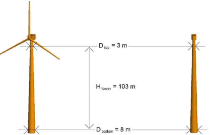
Figure 2.Dimensions of wind turbine (WT) simulation model and simplified rotationally symmetric substitution model (RSSM).
instead of the transmitted angle information used for naviga-tion which is contained in the frequency side bands.
2 Simulation setup
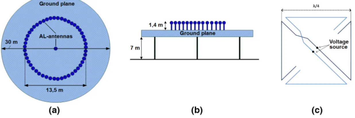
As mentioned in the introduction the omnidirectional car-rier wave of a DVOR surveillance antenna, consisting of 51 Alford Loop (AL) antennas, is used as the source of the simulation setup. Therefor, according to Sandmann et al. (2015), only the center AL antenna of the DVOR model shown in Fig. 3 is fed, whereas the remaining AL antennas are complex-conjugated impedance matched.
While the DVOR antenna is always placed in the origin, the electromagnetic field strength is calculated in a circular volume around the WT, placed in a variable distanceX be-tween 1 and 10 km on the U-axis, as illustrated in Fig. 4. The
unusual placement of the field calculation volume around the WT instead the emitting antenna was chosen expecting the WT’s distortion contribution in an approximately con-stant range along the azimuth, as described more detailed in Sect. 3.3. The calculation points of the field strength in the described volume are arranged in 100 coaxial circles rep-resenting orbit flights (OF) with different radii and heights, marked as intersection points in cross section view in Fig. 5. The overall parametric simulation values for the dis-tanceXof the WT on the U-axis, the rotor diameterD and the angle of wind directionαand rotor positionβaccording to Fig. 1, as well as the OFs’ distancesRand altitudesH, are summarized in Table 1.
The described simulation setup was carried out with all possible combinations of these parameters which corre-sponds to 2080 variations. For all calculations the Multilevel Fast Multipole Method (MLFMM) (van Tonder et al., 2005) of the software tool FEKO (Altair FEKO, 2015) was used. The DVOR and WT models are treated as fully metallic with perfect electrical conductivity.
3 Simulation results and estimation method 3.1 Simulation results
Figure 3.Simulation model of DVOR antenna consisting of 51 Alford Loop antennas.
Table 1.Summary of all parameter values used for simulations.
X 1 km 2 km 3 km 4 km 5 km 6 km 7 km 8 km 9 km 10 km
D 82 m 114 m
α Pos. 1 Pos. 2 Pos. 3 Pos. 4 Pos. 5 Pos. 6 Pos. 7 Pos. 8 Pos. 9 Pos. 10 0◦ 15◦ 30◦ 45◦ 60◦ 75◦ 90◦ 105◦ 120◦ 135◦
α Pos. 11 Pos. 12 Pos. 13 150◦ 165◦ 180◦
β Pos. 1 Pos. 2 Pos. 3 Pos. 4 Pos. 5 Pos. 6 Pos. 7 Pos. 8 0◦ 15◦ 30◦ 45◦ 60◦ 75◦ 90◦ 105◦
R 1 NM 2 NM 3 NM 4 NM 5 NM 6 NM 7 NM 8 NM 9 NM 10 NM
≈ ≈ ≈ ≈ ≈ ≈ ≈ ≈ ≈ ≈
1.8 km 3.7 km 5.6 km 7.4 km 9.3 km 11.1 km 13.0 km 14.8 km 16.7 km 18.5 km
H 1000 ft 2000 ft 3000 ft 4000 ft 5000 ft 6000 ft 7000 ft 8000 ft 9000 ft 10 000 ft
≈ ≈ ≈ ≈ ≈ ≈ ≈ ≈ ≈ ≈
0.3 km 0.6 km 0.9 km 1.2 km 1.5 km 1.8 km 2.1 km 2.4 km 2.7 km 3.0 km
Figure 4.Overview of the simulation setup.
The rising field strength values in the azimuth area of nearly 200◦ are caused by the closeness to the DVOR an-tenna at this region since the beginning of the azimuthγ is defined on the averted part of the U-axis, as shown in Fig. 5.
Figure 5.Illustration of the field strength calculation points ar-ranged in 100 coaxial circles representing orbit flights in cross sec-tion view.
Figure 6.Electric field strength distribution along the azimuth of an orbit flight.
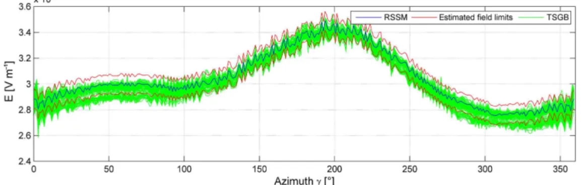
Figure 7.Electric field strength distribution according to Fig. 6 with the appropriate results for the rotationally symmetric substitution model (RSSM) compared with the arithmetic TSGB median.
3.2 Field interval median
Based on the assumption of the rotor blades causing both constructive and destructive interference effects on the field strength while rotating, a median field distribution is as-sumed that is located within the tube shaped graph bundle (TSGB) shown in Fig. 6 and representing the static tower part of WT distortion influence. To ascertain this field distribution the same simulation setup is executed with the rotationally symmetric substitution model (RSSM), shown in Fig. 2, in-stead of the original WT model. The appropriate results show a good compliance with the assumption as exemplary shown in Fig. 7 for the OF with X=1 km, D=82 m, R=6 NM andH=6000 ft comparing with the arithmetic TSGB me-dian.
3.3 Field interval width
Considering all wind direction and rotor position constel-lations, the explanation related to the TSGB median in Sect. 3.2 implicates the width of the TSGB in an approxi-mately constant range along the azimuth γ, while keeping constant the parametersX,D,RandH. At this point the ne-cessity to arrange the OFs coaxial with the WT as a require-ment for this field distribution must be emphasized. Validat-ing this assumption the means and standard deviations of the
TSGB interval widthETSGB_IWover the azimuthγ is
calcu-lated according to Eq. (1), as exemplary shown in Fig. 8 for all OFs with WT distanceX=1 km. Especially for radiiR greater than 1 NM this assumption is verified by the investi-gation. Furthermore, as expected, the TSGB width is higher in case of greater rotor diameterDand is overall falling with rising radiusRwhich confirms the assumption.
ETSGB_IW,γ = |ETSGB_max,γ −ETSGB_min,γ| (1)
ERSSM_IW=
2 360·
360
X
γ=1
|ERSSM,γ −ELFAW,γ| (2)
In order to estimate the TSGB width the averaged RSSM interval width along the azimuthal field distribution is used, since both the RSSM and the WT model are influenced by interference effects of the same manner. Determining the RSSM interval width it is not useful to base the calcula-tion upon some filtering of the field distribucalcula-tion because this method disregards the difference between interference ef-fects and intrinsic signal fractions.
Considering this aspect, the calculation of the averaged RSSM interval widthERSSM_IW is based on the difference
Figure 8.TSGB width means and standard deviations of all OFs with WT distanceX=1 km.
Figure 9.Field distributions for determining RSSM interval widthERSSM_IWaccording to Eq. (2).
RSSM and linearly fitted results of the same simulation setup except for the absence of any WT model (LFAW), as shown in Fig. 9. Due to the average difference betweenERSSM,γ and ELFAW,γ is composed of its absolute values, it has to be du-plicated to determine the full averaged RSSM interval width ERSSM_IW, according to Eq. (2).
Regarding the ratio ETSGB_IW
ERSSM_IW between the WT and RSSM interval widths, as shown in Fig. 10 forX=1 km, it can be stated that the mean values’ range and their standard devia-tions are marginal. Therefor averaged proportionality factors C82=1.70 andC114=1.96 can be deduced by
approxima-tion for both models. As expected, the proporapproxima-tionality fac-torCDis higher in case of greater rotor diameterD.
4 Estimation method
As pointed out in the Sect. 1, for estimation of the electric field distribution in presence of the WT, regularities are used
which are based on the results of 2080 simulation setups with 100 OFs each. Subsequently, these regularities are calibrated by the results of RSSM and LFAW simulation. Thus, only these two simplified simulations need to be carried out for the electric field estimation.
The results of the RSSM simulation provide the es-timated interval median EEST_M. The estimated interval
widthEEST_IW=ERSSM_IW·CDis constructed with both the RSSM and LFAW simulation results, according to Eq. (2), and the proportionality factor CD which slightly depends on the WT rotor reflexion capability affected by the blades length and shape. An exemplary field distribution estimation, created for the used OF (X=1 km, D=82 m, R=6 NM, H=6000 ft, C82=1.70) with this method is shown in
Fig. 11.
Figure 10.Ratio ETSGB_IW
ERSSM_IW between field interval widths of WT model and RSSM forX=1 km.
Figure 11.Field estimation for an exemplary OF and proportionality factorC82=1.70.
Thereby the averaged relative TSGB median estimation error EST_Merr is represented by the error bar median
ac-cording to Eq. (3) while the averaged relative TSGB interval width estimation error EST_IWerris represented by the error
bar width according to Eq. (4). The appropriating averaged values as a function of the WT distance are given in Fig. 13. EST_Merr
= 1
360·
360◦
X
γ=1◦
|EEST_M,γ ,R,H−ETSGB_M,γ ,R,H| ETSGB_IW,γ ,R,H
(3)
EST_IWerr
= 1
360·
360◦
X
γ=1◦
|EEST_IW,γ ,R,H−ETSGB_IW,γ ,R,H|
ETSGB_IW,γ ,R,H
(4)
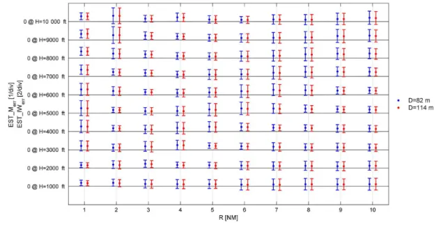
The estimated relative interval width error for the OFs shown in Fig. 12 can be stated with a typical value about 1,
while the estimated relative median error is typically about 1/5 of the interval width. These values can also be distin-guished in Fig. 13 forX=1 km, as this error bar represents the averaged errors of all OFs with thisX value. The ris-ing error bar values with the WT distanceXare constituted by the decreasing TSGB width for higher distances between DVOR and WT, caused by the free space loss. According to Eqs. (3) and (4) this leads to the rising relative error values.
5 Conclusions
Figure 12.Field estimation error for all OFs withX=1 km.
Figure 13.Field estimation error as a function of WT distanceX.
Therefor regularities of the distortion behavior were de-termined by analyzing the simulation results of 2040 non-redundant WT constellations. It was worked out that the tube shaped field graph band width, created by the different WT constellations, is in a steady range provided the distance to the WT is constant. Furthermore, it is ascertained that the field graph band median can be approximated by simulat-ing a blade-less rotationally symmetric substitution model (RSSM) while the field graph band width itself is determined based on the simulation results of the RSSM and linearly fit-ted results of the same simulation setup except for the ab-sence of any WT model.
As a result this method allows to approximate worst case distortion of an omnidirectional emitted electromag-netic field in presence of a WT with the results of only two simplified simulations, which significantly reduces simula-tion effort. The typical overall approximasimula-tion accuracy can be stated with an relative uncertainty below 1/4 of the es-sentially field graph band width for the approximated field graph band median and an appropriate relative uncertainty factor below 1.5 for the field graph band width in regions of insignificant free space loss.
Acknowledgements. We acknowledge support by Deutsche Forschungsgemeinschaft and Open Access Publishing Fund of Leibniz Universität Hannover. Support granted by the Federal Ministry of Economy and Energy according to a resolution by the German Federal Parliament, FKZ: 0325644A-D.
The publication of this article was funded by the open-access fund of Leibniz Universität Hannover.
Edited by: T. Schrader
Reviewed by: J. Bredemeyer and one anonymous referee
References
Altair Engineering GmbH, Calwer Straße 7, 71034 Böblingen, Ger-many, http://www.feko.info, http://www.altair.com, 2015. Bundesverband WindEnergie (BWE),
http://www.wind- energie.de/sites/default/files/attachments/page/arbeitskreis-luftverkehr-und-radar/20131107-bwe-umfrage-radar.pdf (last access: 30 April 2016), 2014.